Cosmic variance of weak lensing surveys in the non-Gaussian regime

Abstract

The results from weak gravitational lensing analyses are subject to a cosmic variance error term that has previously been estimated assuming Gaussian statistics. In this letter we address the issue of estimating cosmic variance errors for weak lensing surveys in the non-Gaussian regime.
Using standard cold dark matter model ray-tracing simulations characterized by $\Omega_{m}=0.3,~{}\Omega_{\Lambda}=0.7,~{}h=0.7,~{}\sigma_{8}=1.0$ for different survey redshifts $z_{s}$, we determine the variance of the two-point shear correlation function measured across 64 independent lines of sight. We compare the measured variance to the variance expected from a random Gaussian field and derive a redshift-dependent non-Gaussian calibration relation.
We find that the ratio between the non-Gaussian and Gaussian variance at 1 arcminute can be as high as $\sim 30$ for a survey with source redshift $z_{s}\sim 0.5$ and $\sim 10$ for $z_{s}\sim 1$. The transition scale $\vartheta_{c}$ above which the ratio is consistent with unity, is found to be $\vartheta_{c}\sim 20$ arcmin for $z_{s}\sim 0.5$ and $\vartheta_{c}\sim 10$ arcmin for $z_{s}\sim 1$. We provide fitting formula to our results permitting the estimation of non-Gaussian cosmic variance errors and discuss the impact on current and future surveys.
A more extensive set of simulations will however be required to investigate the dependence of our results on cosmology, specifically on the amplitude of clustering .

1 Introduction

Weak lensing by large scale structure, i.e. cosmic shear, offers a direct way of investigating the statistical properties of matter in the Universe, without making any assumptions on the relation between dark and luminous matter. Current surveys are large enough to provide high precision constraints on cosmology and the latest measurements performed with the Canada France Hawaii Telescope Legacy Survey [Hoekstra et al. 2006, Semboloni et al. 2006] is a step in that direction. Most of the cosmological constraints from weak lensing use two-point shear statistics [Réfrégier 2003, Van Waerbeke & Mellier 2003], and a crucial step in these cosmological parameter measurements is the estimate of error bars and systematics. Several papers address, statistically, the issue of systematics from E and B modes [Crittenden et al. 2001, Pen et al. 2002, Schneider & Kilbinger 2006], but only few papers address the estimation of cosmic variance of cosmic shear measurements [White & Hu 2000, Cooray & Hu 2001, Schneider et al. 2002]. The latter assumes that the error on the two-point shear correlation function follows Gaussian statistics. However, we know that this is not the case at small scales where non-linear effects become important. Cooray & Hu 2001 use the dark matter halo model in Fourier space to study non-Gaussian covariance. A tentative calibration of this effect on the aperture mass statistic [Van Waerbeke et al. 2002] showed that departure from Gaussianity is expected to occur at angular scales $\lower 2.15277pt\hbox{$\;\buildrel<\over{\sim}\;$}10$ arcminutes. The purpose of this Letter is to estimate the non-linear covariance of the two-point shear correlation function in real space, such that it can be of direct practical use for weak lensing studies, as in Schneider et al. 2002, without having to calculate high order correlation functions semi-analytically. Using ray-tracing simulations for a model close to the concordance cosmological model [Spergel et al. 2006] at different source redshift slices, we obtain a redshift dependent calibration formula of the Gaussian covariance derived in Schneider et al. 2002. This calibration takes the form of a matrix with which the Gaussian covariance is multiplied by, to obtain the non-Gaussian covariance. This letter is organised as follows. The Section 2 provides the notation relevant for this work, and the theoretical description of the Gaussian covariance. Section 3 describes the ray-tracing simulations and Section 4 shows our results. In Section 5 we show their impact on current and future contiguous weak lensing surveys. We conclude by discussing the limitation of our approach and the work that remains to be done in order to achieve percent level accuracy in the non-linear covariance estimate.

2 Cosmic Shear and Covariance

We follow the notation of Schneider et al. 1998. The power spectrum $P_{\kappa}(k)$ of the convergence $\kappa$ is given by

$$P_{\kappa}(k) = {9\over 4}\Omega_{0}^{2}\int_{0}^{w_{H}}{{\rm d}w\over a^{2}(w)}P_{3D}\left({k\over f_{K}(w)};w\right)\times$$ (1)

$$\left[\int_{w}^{w_{H}}{\rm d}w^{\prime}n(w^{\prime}){f_{K}(w^{\prime}-w)\over f_{K}(w^{\prime})}\right]^{2},$$

where $f_{K}(w)$ is the comoving angular diameter distance out to a distance $w$ ($w_{H}$ is the horizon distance), and $n(w(z))$ is the redshift distribution of the sources. $P_{3D}(k)$ is the 3-dimension non-linear mass power spectrum [Peacock & Dodds 1996, Smith et al. 2003], and $k$ is the 2-dimension wave vector perpendicular to the line-of-sight. We are interested in the non-Gaussian covariance of the two-point shear correlation function, because it can be easily transposed to other two-point statistics [Schneider et al. 2002] by a suitable integration in $k$-space. The shear correlation function measured at angular scale $\vartheta$ can be split into two components, $\xi_{\pm}$, where

$$\xi_{\pm}(\vartheta)={1\over 2\pi}\int_{0}^{\infty}{\rm d}k~{}k~{}P_{\kappa}(k)~{}J_{0,4}(k~{}\vartheta),$$ (2)

and $J_{0,4}$ is a Bessel function of the first kind, of zeroth order for $\xi_{+}$ and of fourth order for $\xi_{-}$. The covariance matrix ${\rm Cov(\xi_{+};\vartheta_{1},\vartheta_{2})}$ of the total shear correlation function $\xi_{+}$ can be written as a sum of three different parts:

$${\rm Cov(\xi_{+};\vartheta_{1},\vartheta_{2})} = \langle\xi_{+}(\vartheta_{1})\xi_{+}(\vartheta_{2})\rangle=$$

$$D\delta_{K}(\vartheta_{1}-\vartheta_{2})+q_{++} + <4^{th}\,\rm{order\,correlations}>$$ (3)

The first term is the diagonal statistical noise, depending on the intrinsic ellipticity variance, $\sigma_{e}$, the total area of the survey, $A$, and the density of galaxies, $n$. In practical units gives:

$$D=3.979\times 10^{-9}\Big{(}\frac{\sigma_{e}}{0.3}\Big{)}^{4}\Big{(}\frac{A}{1\,\rm{deg}^{2}}\Big{)}^{-1}\times$$

$$\Big{(}\frac{n}{30\,\rm{arcmin}^{-2}}\Big{)}^{-2}\Big{(}\frac{\theta}{1\,\rm{arcmin}}\Big{)}\Big{(}\frac{\Delta\theta/\theta}{0.1}\Big{)}^{-1}$$ (4)

where $\Delta\theta$ is the bin size used for the sampling of the correlation function. The second term represents the coupling between the noise and two point shear correlation function:

$$q_{++}={2\sigma_{\epsilon}^{2}\over\pi An}\int_{0}^{\pi}{\rm d}\varphi\;\xi_{+}\left(\sqrt{\vartheta_{1}^{2}+\vartheta_{2}^{2}-2\vartheta_{1}\vartheta_{2}\cos\varphi}\right)$$ (5)

and it can easily be calculated using a prediction for non-linear shear power spectrum [Peacock & Dodds 1996, Smith et al. 2003]. The third term requires the knowledge of the fourth order shear correlation function as a function of scale. If we assume Gaussian statistics, it can be expressed as a sum of two terms [Schneider et al. 2002]:

$$r_{+0} = {2\over\pi A}\int_{0}^{\infty}{\rm d}\phi\,\phi\int_{0}^{\pi}\,{\rm d}\varphi_{1}\,\xi_{+}(|{\hbox{$\bf\psi$}}_{a}|)\int_{0}^{\pi}\,{\rm d}\varphi_{2}\,\xi_{+}(|{\hbox{$\bf\psi$}}_{b}|)\;,$$

$$r_{+1} = {1\over(2\pi)A}\int_{0}^{\infty}{\rm d}\phi\,\phi\int_{0}^{2\pi}{\rm d}\varphi_{1}\,\xi_{-}(|{\hbox{$\bf\psi$}}_{a}|)$$

$$\times \int_{0}^{2\pi}{\rm d}\varphi_{2}\,\xi_{-}(|{\hbox{$\bf\psi$}}_{b}|)\left[\cos 4\varphi_{a}\,\cos 4\varphi_{b}+\sin 4\varphi_{a}\,\sin 4\varphi_{b}\right]\;,$$

and $\varphi_{a}$, $\varphi_{b}$ are the polar angles of ${\hbox{$\bf\psi$}}_{a}$, ${\hbox{$\bf\psi$}}_{b}$, respectively, $\cos 4\varphi_{a}=1-8\psi_{a1}^{2}\psi_{a2}^{2}/|{\hbox{$\bf\psi$}}_{a}|^{4}$, $\sin 4\varphi_{a}=4\psi_{a1}\psi_{a2}(\psi_{a1}^{2}-\psi_{a2}^{2})/|{\hbox{$\bf\psi$}}_{a}|^{4}$, and the analogous expressions for $\varphi_{b}$.

In this paper we are interested in the last term of eq. (3). At large scales we know that we can use the Gaussian approximation and write it as the sum of $r_{+0}$ and $r_{+1}$. At small scales the Gaussian statistics break down and this term cannot be calculated with semi-analytical techniques. The rest of the paper discusses our technique to calibrate the Gaussian prediction of this quantity in order to fit the non-Gaussian value measured in ray-tracing simulations. Therefore using ray-tracing simulations, we will measure the covariance of $\xi_{+}$, $\rm{Cov_{measured}(\xi_{+};\vartheta_{1},\vartheta_{2})}$, assuming $\sigma_{e}=0$, so $q_{++}=0$ and $D=0$ and we will define ${\cal F}(\vartheta_{1},\vartheta_{2})$, the ratio between the measured covariance matrix and Gaussian expectation for the covariance matrix:

$${\cal F}(\vartheta_{1},\vartheta_{2})={\rm Cov_{measured}(\xi_{+};\vartheta_{1},\vartheta_{2})\over Cov_{Gaussian}(\xi_{+};\vartheta_{1},\vartheta_{2})}$$ (7)

where ${\rm{Cov_{Gaussian}}}(\xi_{+};\vartheta_{1},\vartheta_{2})=r_{+0}+r_{+1}$.

3 Description of the simulations

We performed 16 particle in mesh (PM) dark matter simulations to cover a light cone of angular size $7\times 7$ degrees, from redshift $z=0$ to $z\simeq 3$, using the tiling technique proposed by White & Hu (2000) and explained in Appendix B of Hamana et al. (2002). We used 7 simulations of size 200 Mpc, 4 of size 400 Mpc, 3 of size 600 Mpc and 2 of size 800 Mpc. Each $N$-body experiment involved $256^{3}$ particles in a grid of size $1024^{3}$ to compute the forces. The cosmology is a standard $\Lambda$CDM model with $\Omega=0.3$, $\Omega_{\rm baryons}=0.04$, $\Lambda=0.7$ and $H_{0}=70$ km/s/Mpc, closed to the concordance model [Spergel et al. 2006], with a slightly higher value for the normalisation $\sigma_{8}=1$. Combining the simulation data in different ways, we generated 64 different, albeit not fully independent (see below), light cones. Each of them is divided in 64 successive redshift planes separated from each other by 100 Mpc. The ray-tracing method is described in Hamana et al. (2002). The spatial resolution of our simulations translates in an angular resolution of the order of $\theta\simeq 0.5$ arcmin for $z\ga 0.2$. Given the limitations of the PM technique, discreteness effects can be significant at redshift $z\ga 1.5$ (due to transcients). Nevertheless, our measurements are reliable at scales larger than the mean interparticle distance, i.e. $\theta\sim 2$ arcmin. and we expect they can still used with high confidence level down to $\theta\simeq 1$ arcmin.

The size, $S$, of our light cones matches closely that of the simulations, so using the dispersion among them to compute the covariance matrix would certainly underestimate its amplitude, even at small angular scales. Fluctuations at scales larger than the simulation box size are also missed with these realisations. Furthermore, they are not strictly independent, since they just combine in different ways the 20 simulations. For these two reasons, in the case of $A=S$ the value of ${\cal F}(\vartheta_{1},\vartheta_{2})$ on small scales would be always underestimated, as compared to the cases $A\neq S$, and would not converge to unity at large scales. In order to minimise these limitations and still have a fair estimate of the covariance matrix on the estimator used here, it is thus wise to always keep the angular size of the survey $A$ to a small fraction of $S$. In practice, we divide $S$ in 4, 9 and 16 adjacent subsamples, leading to assumed values of $A\simeq 12$, $5.4$ and $3.1$ square degrees and 256, 576, 1024 realisations respectively, in total. Note that the choice of $A$ is made such that the largest angular scale considered, $\theta=20$ arcmin, remains small compared to $\sqrt{A}$. We finally choose $A=5.44~{}{\rm deg^{2}}$.

4 Description of the matrix calibration

We measure ${\cal F}(\vartheta_{1},\vartheta_{2})$ according to eq. (7) as follows. The term ${\rm Cov_{measured}(\xi_{+};\vartheta_{1},\vartheta_{2})}$ is given by $\langle(\xi_{+}-\langle\xi_{+}\rangle)^{2}\rangle$, where $\xi_{+}$ is measured in each realisation of the survey of size $A=5.44~{}{\rm deg^{2}}$, while the average $\langle\cdots\rangle$ is performed over all the realisations. The term ${\rm Cov_{Gaussian}(\xi_{+};\vartheta_{1},\vartheta_{2})}$ is calculated by measuring $\xi_{+}$ and $\xi_{-}$ in the 64 largest samples $S$ of area $A=49\ {\rm deg}^{2}$, and integrating numerically eqs. (2). This ensures that the numerator and denominator in eq. (7) are self-consistently defined. It is worth noticing that for all cases with $A<S$ the asymptotic behavior of ${\mathcal{F}}(\vartheta_{1},\vartheta_{2})$ does not converge to unity. It indeed seems to be even worse than for the case $A=S$. This is a well-known effect which occurs when the scales become comparable to the size of the survey (Peebles 1974). The result is that for those scales the measured shear correlation is biased to lower values. Therefore, at small scales, the measured cosmic variance ${\rm Cov_{measured}(\xi_{+};\vartheta_{1},\vartheta_{2})}$, when $A<S$ , is more biased low and decreases faster when the scale increases than for the case ${\rm Cov_{Gaussian}(\xi_{+};\vartheta_{1},\vartheta_{2})}$ and $A=S$. The final result is that the ratio ${\mathcal{F}}(\vartheta_{1},\vartheta_{2})$ becomes smaller than unity. Note that in practice, for numerical reasons we have to use $A=S$ to compute ${\rm Cov_{Gaussian}(\xi_{+};\vartheta_{1},\vartheta_{2})}$ using 2. We do not expect this has any impact on our results, within the level of accuracy we can achieve from this set of simulations, provided we rescale the covariance matrix only in the inner part.

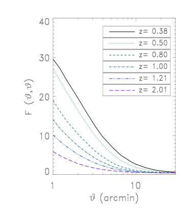
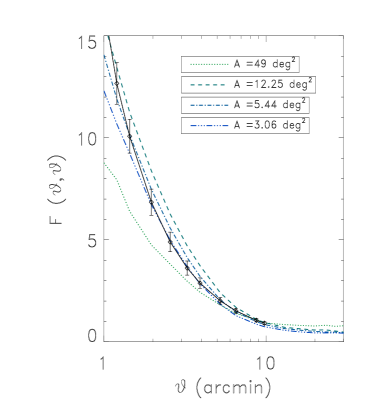
Figure 1: Left panel: Diagonal elements of the matrix ${\cal F}(\vartheta_{1},\vartheta_{2})$ for different source redshift planes. Right panel: Diagonal elements ${\cal F}(\vartheta_{1},\vartheta_{2})$ for different survey sizes and $z_{s}=1$. The black solid line represents the best-fit of ${\cal F}(\vartheta_{1},\vartheta_{2})$ using eq. (8). Error bars are computed using bootstrap with $1000$ realisations.

Figure 2: The plots shows the measured parameters $\alpha$, $\beta$ and $\vartheta_{c}$ of the calibration matrix (see eq. 8) as a function of the redshift. Error bars are computed using bootstrap with 1000 realisations. The solid line shows the best fit from eq. (4).

The left panel of Fig.1 shows the diagonal elements ${\cal F}(\vartheta_{1},\vartheta_{2})$ for different source redshifts. For a source redshift ${\rm z_{s}}\simeq 1$ the calibration factor is $\sim 10$ at $\vartheta_{1}=\vartheta_{2}=1$ arcmin, implying that the cosmic variance has been widely underestimated in previous lensing surveys at scales below $\sim 10$ arcminutes. The correction factor is larger for lower source redshifts. The transition scale $\vartheta_{c}$, which defines the angular scale transition from Gaussian and non-Gaussian covariance, is redshift dependent because the non-linear regime starts at larger scales for nearby structures. Therefore, the calibration matrix must be parameterized with an explicit redshift dependence. We choose a generic power law behavior, as suggested by the left panel of Fig. 1, to parameterize ${\cal F}(\vartheta_{1},\vartheta_{2})$:

$${\cal F}(\vartheta_{1},\vartheta_{2})={\alpha(z)\over\left[\vartheta_{1}\vartheta_{2}\right]^{\beta(z)}}.$$ (8)

The two panels in Fig. 2 show $\alpha$ and $\beta$ as measured in the ray-tracing simulations at nine different source redshifts $z_{s}=[0.4,0.5,0.8,1.0,1.2,1.4,1.5,2.0,3.0]$. These measurements are well fit by the following redshift dependent functions:

$$\alpha(z) = {a_{1}\over z^{a_{2}}}+a_{3}$$

$$\beta(z) = b_{1}~{}z^{b_{2}}~{}{\rm exp}(-z^{b_{3}})+b_{4}.$$ (9)

For $\alpha$, we find $(a_{1},a_{2},a_{3})=(16.90,0.95,-2.19)$, and for $\beta$, $(b_{1},b_{2},b_{3},b_{4})=(1.62,-0.68,-0.68,-0.03)$ in the samples with angular size $A=5.4\ {\rm deg}^{2}$. The fit is performed on scales below $10$ arcminutes, which allows us to define also the transition angle $\vartheta_{c}$ as the scale where the fitted function crosses the Gaussian covariance. The third panel of Fig. 2 represents the measurement of $\vartheta_{c}$. Using the same functional form as for $\alpha$, namely $\vartheta_{c}={t_{1}\over z^{t_{2}}}+t_{3}$, We find the best fit values $(t_{1},t_{2},t_{3})=(8.07,0.95,1.65)$.

Since the normalisation of our simulations is high ($\sigma_{8}=1$), we expect $\vartheta_{c}$ to be slightly overestimated. Several other sources of uncertainty in our measurements may also spoil the estimate of the covariance. In particular, as previously anticipated, there is also a “cosmic error” and a ”cosmic bias” that affect our measurements (e.g. Szapudi & Colombi 1996), which are difficult to estimate. Fortunately, such a cosmic bias/error is expected to increase with the survey size $A$. According to eq. (2), the covariance scales as $\propto 1/A$, so ${\cal F}$ should in fact be independent of $A$, which allows one to use our parametrisation of ${\cal F}$ for any (reasonable) angular survey size. This property can also be used to check the convergence between our realisations of various survey sizes as illustrated by right panel of Fig. 1. Surveys with areas $A=3.1$, $5.4$ and $12$ square degrees agree with each other, but there is a problem with $A=49\ {\rm deg}^{2}$, where ${\cal F}$ is biased low. In the latter case, this is not surprising since the light cone size is comparable to the simulations size, as discussed in § 3. The convergence between other values of $A$ suggest that the cosmic bias/error on ${\cal F}$ measured in these samples is small, i.e. the full set $S$ from which they are extracted, is a fair enough sample. We check this by dividing our $A=12\ {\rm deg}^{2}$ set of 256 realisations into 4 subsamples of 64 realisations, and measured ${\cal F}$ in each of the subsamples. The dispersion between these 4 subsamples is of the order of 10% - 20%, which gives a rough idea of the accuracy of our estimate of ${\cal F}(\vartheta,\vartheta)$, in agreement as well with the convergence between the measurements observed on right panel of Fig. 1 for $A\leq 12\ {\rm deg}^{2}$.

While our choice of parametrisation eq. (8) is globally accurate to $\sim 20\%$ along the diagonal of the matrix ${\cal F}(\vartheta_{1},\vartheta_{2})$, it becomes less accurate for very different $\vartheta_{1}$ and $\vartheta_{2}$. One should note that the lack of accuracy in the off diagonal components is not critical because the cross-correlation coefficient is $\lower 2.15277pt\hbox{$\;\buildrel<\over{\sim}\;$}0.1$ in this region.

5 Impact of non-Gaussianity on current and future Surveys

Finally, we compare the amplitude of statistical and cosmic variance at small scales for a range of contiguous surveys such as GEMS [Heymans et al. 2005], COSMOS (Massey et al. in prep. ), CFHTLS Wide [Hoekstra et al. 2006] and two different versions of SNAP [Réfrégier et al. 2004] whose characteristics are shown in table 1. The statistical noise is computed using eq. (4) , assuming a bin size $\Delta\theta=0.1$. Note that the statistical noise differs if the bin size used to measure the correlation function is different. In addition we choose $\sigma_{e}=0.4$ for ground-based surveys and $\sigma_{e}=0.3$ for space-based surveys. Fig. 3 shows that by dropping the Gaussian approximation the total noise changes at small scales. The changing due to the non-Gaussian correction depends on the relative amplitude of the three different contributions to the total variance, namely, the shot noise, the sampling noise and the coupling term. For “low density” surveys, such as the CFHTLS Wide, the impact of the non-Gaussian correction is smaller as compared to the one expected for the low noise space based surveys, where the cosmic variance far exceeds the statistical noise. It is worth noticing our results are obtained for a higher $\sigma_{8}$ value than Spergel et al. 2006 ($\sigma_{8}\simeq 0.75$) and are likely to be slightly different for this model. A more extensive analysis of simulations made with different cosmologies would be necessary to accurately predict the amplitudes of the non-Gaussianity corrections to the cosmic variance.

Table 1: Main Characteristics of surveys used in Fig. 3.

Name	A ($\rm{deg}^{2}$)	n	$<z_{s}>$
GEMS	$0.25$	$65$	$1$
COSMOS	$1.6$	$80$	$1.2$
CFHTLS Wide	$50$	$15$	$0.8$
$\rm{SNAP\,deep}$	$15$	$300$	$1.4$
$\rm{SNAP\,wide}$	$260$	$120$	$1.2$

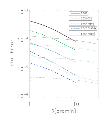
Figure 3: The total, statistical plus cosmic variance noise for each survey of table 1. The noise including the non-Gaussian correction (thick lines) is compared on scales $\vartheta\leq 10$ arcmin, with the noise expected in the case of Gaussian statistics (thin lines). Dropping the Gaussian assumption increases noise on small scales. The impact of the non-Gaussian correction for the CFHTLS Wide is small; the statistical noise $\propto 1/n^{2}$ and the coupling term $q_{++}\propto 1/n$ still dominates at small scales for such a density. These same terms become negligible for the space based surveys whose density is much higher.

Unfortunately, only a small set of $\Lambda CDM$ ray tracing simulations with $\sigma_{8}=0.8$ is available. This set of simulations, whose characteristics are given in Heymans et al. 2006, is composed of two redshift planes each containing 12 simulations of $25~{}{\rm deg^{2}}$ which is not enough to find a recalibration fitting formula. Nevertheless, Fig.4 shows that even for a $\Lambda CDM$ model with $\sigma_{8}=0.8$ the cosmic variance has been widely underestimated. Fig.4 also shows that using a rescaling obtained from $\sigma_{8}=1.0$ gives results which are in good agreement with the ones obtained for $\sigma_{8}=0.8$ for low redshift surveys and slightly overestimates the cosmic variance as the depth increases. These simulations were also used to confirm the validity of our statements regarding the behavior of the ratio ${\mathcal{F}}(\vartheta_{2},\vartheta_{2})$ and the change of the size of $A$ used for the recalibration.

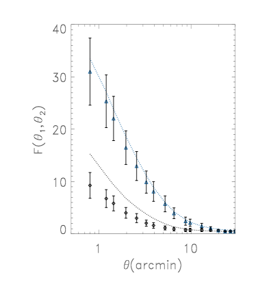
Figure 4: Diagonal elements of the matrix ${\cal F}(\vartheta_{1},\vartheta_{2})$ for planes with $z_{s}\simeq 0.5$ (blue triangles) and $z_{s}\simeq 1$ (black diamonds) obtained for the set of simulations $\Lambda CDM$ with $\sigma_{8}=0.8$. Error bars are obtained using bootstrap with $1000$ realisations. For each of the two measurements we compare the obtained value with the predicted value calculated from $\Lambda CDM$ simulations with $\sigma_{8}=1.$, marked with black and blue dotted lines.

6 Discussion and Conclusion

We have shown that the non-Gaussian contribution to the covariance in two-point shear statistics cannot be neglected at small angular scales. Using ray-tracing simulations we have calibrated the non-Gaussian covariance with respect to the Gaussian covariance as calculated in Schneider et al. 2002. We have derived a calibration matrix which can be used as a first approximation for cosmological parameter measurements in current lensing surveys and for parameter forecasting.

We found that the correction coefficient could be as high $10$ at $1$ arcminute for a source redshift of $1$, and $30$ for source redshift of $z_{s}=0.5$. The transition between Gaussian and non-Gaussian covariance occurs around $10$ arcminutes for $z_{s}=1$ and $20$ arcminutes for $z_{s}=0.5$. Our work shows that it is important to include this non-Gaussian contribution to the shear estimated errors, and that sub-arcminute resolution ray-tracing simulations are very useful for this purpose. Although this source of error has been neglected in previous lensing analysis, we note that it should not strongly impact the measurement of $\sigma_{8}$ for surveys using the shear signal measured above the transition scale $\vartheta_{c}$, where the Gaussian covariance is a reasonable assumption. However, it will significantly affect the joined $\Omega_{M}$-$\sigma_{8}$ constraints, since the degeneracy breaking between these two parameters is based on a the relative amplitude of the shear correlation signal between small and large scales [Jain & Seljak 1997]. An increased error at small scale, as shown here, will make the degeneracy more difficult to break.

Extension of this work via a thorough analysis of the non-Gaussian covariance based on numerical simulations include shear error calibration with broad redshift distribution (tomography), different two-points statistics and the dependence of the non-Gaussian correction with a varying cosmology. In particular we expect a non-trivial dependence of the calibration matrix with $\sigma_{8}$, since, for a fixed angular scale, non-linear structures form earlier for higher $\sigma_{8}$.

References

- [Cooray & Hu 2001] Cooray, A., Hu, W., 2001, ApJ, 554, 66
- [Crittenden et al. 2001] Crittenden, R., Robert, G., Natarajan, P., Pen, U. L. , Theuns, T., 2001, ApJ, 568, 20
- [Hamana et al. 2002] Hamana, T., Colombi, S., Thion, A., Devriendt, J., Mellier, Y., Bernardeau, F., 2002, MNRAS, 330, 365
- [Heymans et al. 2005] Heymans, C.,White, M., Heavens, A., Vale, C., van Waerbeke, L.,2005, MNRAS, 361, 160
- [Heymans et al. 2006] Heymans, C. et al., 2006, MNRAS, 371, 750
- [Hoekstra et al. 2006] Hoekstra, H,et al., 2006, ApJ, 647, 166
- [Jain & Seljak 1997] Jain, B., Seljak, U., 1997, ApJ, 484, 560
- [Peacock & Dodds 1996] Peacock, J.A., Dodds, S.J., 1996, MNRAS, 280, L9
- [Peebles 1974] Peebles, P.J.E., 1974, A&A, 32, 197
- [Pen et al. 2002] Pen, U.L., van Waerbeke, L., Mellier, Y., 2002, ApJ, 567, 31
- [Réfrégier 2003] Réfrégier, A., 2003,ARAA, 41, 645
- [Réfrégier et al. 2004] Réfrégier, A. et al., 2004, AJ, 127, 3102
- [Schneider & Kilbinger 2006] Schneider, P., Kilbinger, M., 2006, astro-ph/0605084
- [Schneider et al. 1998] Schneider, P.,van Waerbeke, L., Kilbinger, M., Mellier, Y., 1998, MNRAS, 296, 873
- [Schneider et al. 2002] Schneider, P.,van Waerbeke, L., Jain, B., Kruse, G., 2002, A& A, 396, 1
- [Semboloni et al. 2006] Semboloni, E. et al., 2006, A& A, 452, 51
- [Smith et al. 2003] Smith R. E. et al., 2003, MNRAS, 341, 1311
- [Spergel et al. 2006] Spergel D. N., et al. 2006, astro-ph/0603449
- [Szapudi & Colombi 1996] Szapudi, I., Colombi, S., 1996, ApJ, 470, 131
- [Van Waerbeke & Mellier 2003] Van Waerbeke, L., Mellier, Y., 2003, astro-ph/0305089
- [Van Waerbeke et al. 2002] Van Waerbeke, L, Mellier, Y., Pelló, R, Pen, U. L., McCracken, H. J., Jain, B., 2002, A& A, 393, 369
- [White & Hu 2000] White, M., Hu, W., 2000, ApJ, 537, 1