Synchrotron flaring in the jet of 3C 279

Abstract

Aims. We study the synchrotron flaring behaviour of the blazar 3C 279 based on an extensive dataset covering 10 years of monitoring at 19 different frequencies in the radio-to-optical range.

Methods. The properties of a typical outburst are derived from the observations by decomposing the 19 lightcurves into a series of self-similar events. This analysis is achieved by fitting all data simultaneously to a succession of outbursts defined according to the shock-in-jet model of Marscher & Gear (1985).

Results. We compare the derived properties of the synchrotron outbursts in 3C 279 to those obtained with a similar method for the quasar 3C 273. It is argued that differences in the flaring behaviour of these two sources are intrinsic to the sources themselves rather than being due to orientation effects. We also compare the start times and flux densities of our modelled outbursts with those measured from radio components identified in Very Long Baseline Interferometry (VLBI) images. We find VLBI counterparts for most of our model outbursts, although some high-frequency peaking events are not seen in the radio maps. Finally, we study the link between the appearance of a new synchrotron component and the EGRET gamma-ray state of the source at 10 different epochs. We find that an early-stage shock component is always present during high gamma-ray states, while in low gamma-ray states the time since the onset of the last synchrotron outburst is significantly longer. This statistically significant correlation supports the idea that gamma-ray flares are associated with the early stages of shock components propagating in the jet. We note, however, that the shock wave is already beyond the broad line region during the gamma-ray flaring.

1 Introduction

It is generally accepted that radio outbursts in active galactic nuclei (AGN) are triggered by growing shocks in a relativistic jet. There have been many efforts to identify the individual components in radio to submillimeter (submm) lightcurves. Litchfield et al. (1995) and Stevens et al. (1995, 1996, 1998) managed to follow the early evolution of individual outbursts by subtracting the quiescent contribution (assumed to be constant) from the total spectrum. Valtaoja et al. (1999) identified outbursts by decomposing the variations in millimeter (mm) and centimeter lightcurves into exponential flares. Türler et al. (1999) measured the properties of synchrotron outbursts by decomposing the radio-to-submillimeter wavelength lightcurves into a series of self-similar flaring events. The method was further developed by Türler et al. (2000) who used the shock model of Marscher & Gear (1985) to describe both the average evolution of the outbursts and their individual characteristics. This model was found to provide a good description of the lightcurves of 3C 273. In this work, we decompose the lightcurves of a second source, 3C 279. Since our adopted methodology is analogous to that used by Türler et al. (2000) the results are directly comparable to those found for 3C 273.

While in previous studies the outbursts were identified in the radio-to-submillimeter regime, we here follow the synchrotron spectrum up to infrared and optical frequencies. Searches for correlations in the radio-to-optical emission from AGN have been conducted since the 1970s. One of the most recent works was presented in Hanski et al. (2002). In their sample of 20 AGNs they found a clear radio-to-optical correlation in seven cases, a possible correlation in six cases and no correlation for the remainder. This agrees well with the findings of previous studies: there appears to be some kind of correlation between the radio and optical emission but this correlation is not seen in all sources at all epochs. The general trend seems to be that all radio outbursts are accompanied by optical outbursts but conversely not all optical outbursts have radio counterparts.

The source 3C 279 is one of the brightest and most variable blazars at radio wavelengths. As such, it is monitored regularly in all radio wavebands from the centimeter to the submillimeter domain. In the optical, the historical lightcurve shows variations with a typical amplitude of about 2 magnitudes, but reaching 8 magnitudes during flares (Webb et al. 1990). The weak blue bump of 3C 279 allows us to follow the synchrotron spectrum up to infrared and optical wavelengths. Indeed, 3C 279 is one of the few objects for which a clear correlation is found between the radio and optical wavebands (Tornikoski et al. 1994).

In this paper we present results of a multifrequency lightcurve decomposition of 3C 279. The method used is based on Türler et al. (1999; 2000) with some modifications for the specific case of 3C 279, including an extension of the analysis to infrared and optical wavelengths. The average evolution of outbursts is compared to that of 3C 273. We also compare our results with (1) VLBI maps from Wehrle et al. (2001) and Jorstad et al. (2004) to study the connection between the model outbursts and VLBI components, and (2) gamma-ray data obtained by Hartman et al. (2001) to study the connection between the synchrotron spectra and the gamma-ray state.

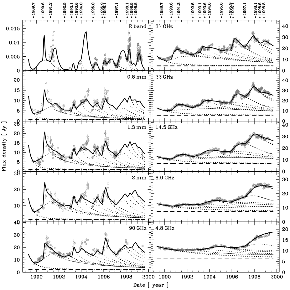
Figure 1: Ten out of nineteen radio-to-optical lightcurves of 3C 279. The points indicate the observed flux density and the solid line our best fit which is a sum of the underlying jet (long dashed line) and the fifteen outbursts (dotted lines). The first dotted line represents the global decay of all outbursts peaking before 1989.0

2 Data

To decompose the radio-to-optical lightcurves of 3C 279 we used data from five radio and seven mm/submm wavelengths as well as four infrared and two optical wavebands. The data sample extends from 1989.0 to 1999.5.

The 4.8, 8.0 and 14.5 GHz data are from the University of Michigan Radio Astronomy Observatory (UMRAO). Some of these data have not previously been published. The 22 and 37 GHz data and some of the 90 GHz data are from the Metsähovi Radio Observatory. These data were published by Teräsranta et al. (1998, 2004). We have also used 90 and 230 GHz (1.3 mm) data from the Swedish-ESO Sub-millimeter Telescope (SEST). SEST data taken prior to 1994.5 were published by Tornikoski et al. (1996) while more recent data are published here for the first time. From the Institut de Radio Astronomie Millimétrique (IRAM) we have data at 90, 150 and 230 GHz (Steppe et al. 1993; Reuter et al. 1997). We also used data at 2.0, 1.3, 1.1, 0.85, 0.8, 0.45 and 0.35 mm from the James Clerk Maxwell Telescope (JCMT). The 0.85 mm dataset was published by Robson et al. (2001) while data in the other wavebands are either from Stevens et al. (1994) or are previously unpublished (post 1993). The dataset of Stevens et al. (1994) also includes the four infrared wavebands used in this work.

The optical R- and V-band lightcurves are collected from the literature, but also contain previously unpublished data. We have used the data from Maraschi et al. (1994), Hartman et al. (1996), Villata et al. (1997), Katajainen et al. (2000) and Hartman et al. (2001). The previously unpublished data are from the Kungliga Vetenskapsakademien (KVA) telescope and the Nordic Optical Telescope (NOT) as well as from the observatories of Perugia and Torino.

3 Model and Method

In this paper we study the multifrequency lightcurves of 3C 279 in the context of the shock model of Marscher & Gear (1985). As the shock propagates downstream in the relativistic jet it evolves through three stages. In the initial (growth) stage, when inverse Compton losses predominate, the synchrotron self-absorption turnover frequency decreases and the turnover flux density increases. In the second (plateau) stage, synchrotron losses dominate and the turnover frequency decreases while the turnover flux density remains roughly constant. During the third (decay) stage when adiabatic losses dominate, both turnover frequency and turnover flux density decrease.

Bjornsson & Aslaksen (2000) criticize one of the assumptions of Marscher & Gear (1985) which concerns the rise of the peak flux density during the initial Compton stage. Their correction of the expression for the energy density of synchrotron photons implies a much shallower rise of peak flux density with peak frequency at the beginning of the outburst. On the other hand, multiple Compton scattering, a process not considered by Marscher & Gear (1985), would actually steepen their derived relation. There is therefore no compelling theoretical reason to use a modified version of the original Marscher & Gear (1985) model.

In Türler et al. (2000), a generalisation of this model was used to decompose the multifrequency lightcurves of 3C 273. We adopt a similar methodology in this work. The shape of the emission spectrum behind the shock front is assumed to be that of a simple synchrotron spectrum (with electron energy distribution $N(E)\propto KE^{-s}$) with two spectral breaks, namely the low-frequency break, $\nu_{\mathrm{h}}$, below which $\alpha_{\mathrm{thick}}=5/2$ and the high frequency break, $\nu_{\mathrm{b}}$, which steepens $\alpha_{\mathrm{thin}}$ from $(1-s)/2$ to $-s/2$. To extend the decomposition into the infrared and optical we introduce an additional high frequency exponential cut-off to the synchrotron spectrum corresponding to emission from the most energetic electrons. The sharp low- and high-frequency spectral breaks of Türler et al. (2000) were also replaced by more realistic smooth transitions. As in the modelling of the micro-quasar GRS 1915+105 (Türler et al. 2004), we introduced a new parameter allowing the ratio $\nu_{\mathrm{h}}/\nu_{\mathrm{m}}$ of the low-frequency spectral break, $\nu_{\mathrm{h}}$, and the synchrotron self-absorption turnover, $\nu_{\mathrm{m}}$, to vary with time.

Another significant change is the addition of an underlying jet component with constant flux density. This component is assumed to be an inhomogeneous synchrotron source with a spectrum defined by a high-frequency break fixed at 375 GHz – as suggested by the quiescent level studies of 3C 279 (Litchfield et al. 1995) – and by two free parameters of the fit defining the synchrotron self-absorption flux density and frequency. To be consistent with the lowest infrared measurements an exponential cut-off was also added to the underlying jet spectrum at a somewhat arbitrary frequency of 2$\cdot 10^{5}$ GHz. We note, however, that our conclusions are insensitive to these numerical values.

The specificity of the individual outbursts is modelled by varying the scale of their evolution in flux density, frequency and time as done in Türler et al. (1999). The more physical approach adopted by Türler et al. (2000) of varying the onset values of $K$ (electron energy density normalization), $B$ (magnetic field strength) and $D$ (Doppler factor) was also tried, but was found to limit the differences between outbursts too much to get an equally good fit.

The model presented here assumes a constant Doppler factor $D\propto R^{-d}$ and a magnetic field $B\propto R^{-b}$ perpendicular to the jet axis as suggested by VLBI polarization measurements (Lister et al. 1998, Marscher et al. 2002). The exponents, $b$ and $d$, of the evolution of these quantities with radius, $R$, of the jet are therefore fixed to $d=0$ and $b=1$. We tried varying these values as well, but this did not result in significantly better fits.

The resulting model has a total of 77 free parameters to fit the 15 outbursts identified in the lightcurves of 3C 279 from 1989 to 2000. Twelve parameters are used to describe the shape and evolution of the synchrotron spectrum for an average outburst. Three further parameters describe the initial flux density decay while two are needed to describe the underlying jet component. The remaining 60 parameters are used to describe the start time and the specific characteristics of the 15 different outbursts. The total number of degrees of freedom is 3281.

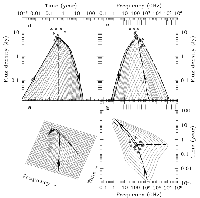
Figure 2: Logarithmic evolution of the synchrotron emission of an average outburst in 3C 279. The three dimensional (log $\nu$, log $S$, log $t$) representation is shown in (a), while the Cartesian projections of this surface are shown in (b), (c) and (d). b) Frequency versus time representation with contours starting at a flux density of 0.02 Jy and spaced by 0.3 dex. c) The synchrotron spectra at different times spaced by 0.2 dex. d) The lightcurves at different frequencies spaced by 0.2 dex. The thick solid line with arrows traces the time evolution of the spectral turnover, whereas the dashed line connects the peak of the lightcurves at different frequencies. The filled circles refer to the specific characteristics of the outbursts (see Section 4.2) and the vertical bars in (b) and (c) show the frequency coverage of the 19 lightcurves.

4 Results

The best-fit decomposition of the radio-to-optical lightcurves into a series of 15 self-similar outbursts is shown in Fig. 1. It has a reduced $\chi^{2}$ value of 8.72. This relatively high value can be considered as acceptable here keeping in mind that the aim of the modelling is to derive the average properties of a typical outburst and that the specificity of each outburst is only modelled very crudely in order to minimise the number of free parameters. Furthermore, the analytical shock-in-jet model itself is of necessity a simplistic idealization of the complex emission of actual jets (Gómez 2005) and thus a perfect match of the model to the data cannot be expected. At the lowest frequencies, the fit describes the smooth shape of the lightcurves very well. At 90 GHz, the general flux density level of the fit is good, but during the biggest outbursts (in 1991, 1993.5, 1994 and 1996.5) the model flux density remains below the observations. The same tendency also applies to all mm-band lightcurves and to the optical R- and V-band lightcurves. Part of this fit (until 1994.0) has been published in Lindfors et al. (2005).

4.1 Average evolution of the synchrotron spectrum

The average evolution of an outburst in 3C 279, as defined by 12 fit parameters, is shown in Fig. 2. In Fig. 2c we see the average outburst spectra. It peaks at $\sim$150 GHz, which is the frequency at which the transition from the Compton stage to the synchrotron stage takes place. The peak flux density is 6.6 Jy. The second stage transition in the average spectra is at $\sim 20$ GHz and its flux density is 2.2 Jy.

The overall shape of the evolution is quite different from the one derived for 3C 273 (Türler et al. 2000). The most obvious difference is the decreasing flux density during the second stage of the evolution which is quite different from the typical plateau seen in 3C 273. In the model, this difference can be ascribed to the high value of the parameter $k$ defining the decrease of the normalization $K\propto R^{-k}$ of the electron energy distribution $N(E)\propto K\,E^{-s}$ with jet opening radius, $R$. The derived value of $k$ is $4.0$ which is far above the value of $k_{\mathrm{ad}}=2(s+2)/3=2.81$ (with $s=2.25$) predicted for an adiabatic jet flow. The original Marscher & Gear model adopted only adiabatic compression to heat the electrons in the shock. While this seems to be a good assumption for 3C 273 (k=3.03), our high $k$-value found for 3C 279 suggests that the emitting electrons are subject to important non-adiabatic cooling processes within the jet. This might be due, at least in part, to synchrotron and inverse Compton radiative losses in the undisturbed underlying jet.

As mentioned in Türler et al. (2000), the three parameters $r$, $k$ and $d$ are difficult to constrain uniquely by the fit. In particular, the effect of $k>k_{ad}$ and of $d>0$ are similar, both producing a decreasing flux density during the synchrotron stage of the evolution. The high value of $k$ might therefore also indicate that our assumption of $d=0$ is not valid and thus suggest that the Doppler factor tends to decrease during the evolution of the shock. This could be due to a decelerating jet flow or to a geometry in which the jet bends away from the line of sight (see Jorstad et al. 2004).

Another difference is that the flattening of the spectral index by $\Delta\alpha_{thin}=+0.5$ (predicted to occur at the synchrotron-to-adiabatic stage transition) is found to be much less abrupt for 3C 279 than for 3C 273, and for 3C 279 it starts much earlier during the initial Compton stage. This can be seen by the position of the start of the flattening ($t_{\mathrm{f}}$) in Fig. 3, which is much earlier than found for 3C 273 (see Fig. 4. of Türler et al. (2000)). A similar behaviour was also found for GRS 1915+105 (Türler et al. 2004).

Apart from $k$, the values of two other physical parameters of the jet are found to be similar to those derived for 3C 273 (Türler et al. 2000). The index, $s$, of the electron energy distribution is found here to be $s=2.25$ ($s=2.05$ for 3C 273) and the opening radius $R\propto L^{r}$ of the jet with distance, $L$, along the flow is found to be slightly non-linear ($r=0.78$) indicating that, as for 3C 273 ($r=0.8$), the jet opening angle is slowly decreasing with distance suggesting that some jet collimation process is at work.

We also note, as was found for GRS 1915+105 (Türler et al. 2004), that there is a tendency for the synchrotron emission of the outbursts to start out inhomogeneous but to become homogeneous as the shock evolves with time. This is manifested as a decreasing $\nu_{\mathrm{h}}/\nu_{\mathrm{m}}$ ratio which affects the shape of the spectrum at frequencies below the turnover as can be seen in Fig. 2c.

Another difference is that in 3C 273 the outbursts are very short-lived at higher frequencies, while in 3C 279 at all frequencies above $\sim$150 GHz it takes $\sim$ 0.45 years to reach the peak flux density. Since the rise time at all such high frequencies is the same these outbursts peak simultaneously. This is shown in Fig. 3. This result, together with the finding that the plateau stage is a bit shorter than in 3C 273, might suggest that in 3C 279 the magnetic field energy density is relatively lower than the electron energy density.

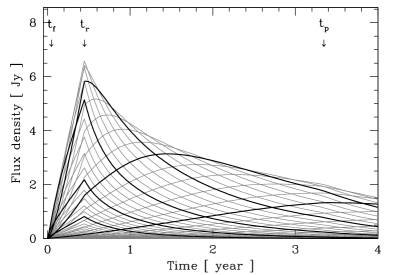
Figure 3: Model lightcurves of the average outburst in 3C 279 at different frequencies spaced by 0.1 dex (grey lines). The six highlighted lightcurves are at frequencies, $\nu$, defined by log($\nu$/GHz)= 3.5, 2.5,…,1.0, in order of increasing timescales. t_r and t_p refer to transitions from Compton to synchrotron stage (t${}_{\mathrm{r}}=$0.45 years) and from synchrotron to adiabatic stage (t${}_{\mathrm{p}}=$3.34 years) respectively. t_f refers to the time when the flattening of the spectral index starts (t${}_{\mathrm{f}}=$0.046 years).

3C 279 is an archetypical blazar while 3C 273 is not a true member of the blazar class. Most conspicuously, it is not rapidly variable in the optical band and has low optical polarization. However, it exhibits blazar-like optical behaviour at low levels, diluted by thermal radiation (Impey et al. 1989, Valtaoja et al. 1990, Valtaoja et al. 1991) and has therefore been dubbed a mini-blazar by Impey et al. (1989). As expected within the context of the unification scheme, 3C 273 has a rather large viewing angle, estimated to be around 10 degrees (Lähteenmäki & Valtaoja 1999, Savolainen et al. 2006). This is smaller than for ordinary quasars, but larger than for blazars; for 3C 279 the estimated viewing angle is around 2 degrees (Lindfors et al. 2005 and references therein).

In the simplest unification models, orientation is the only parameter. One might therefore expect that the borderline blazar 3C 273 would appear similar to 3C 279 if the viewing angle were decreased. However, some of the differences we find between 3C 273 and 3C 279 (non-adiabatic jet flow in 3C 279, adiabatic in 3C 273; magnetic energy density lower than electron energy density in 3C 279 whereas in 3C 273 there is little difference) seem intrinsic to the sources and cannot be explained by differences in viewing angles alone. However, we note that variations in the viewing angle as a function of time/radial distance could play a role in the observed differences between these two sources.

4.2 Characteristics of Different Outbursts

The evolution of each of the 15 individual outbursts is allowed to deviate in scale from the average outburst. For this we need three parameters corresponding to the logarithmic shifts along the three axes of Fig. 2, namely time, $\Delta\log t$, frequency, $\Delta\log\nu$ and flux density, $\Delta\log S$. The values obtained for these shifts are given in Table 1 and their distribution is shown graphically with the filled circles in Fig. 2.

Shock nr.	$T_{0}$	$\Delta$ log$S$	$\Delta$ log$\nu$	$\Delta$ log$t$
1	1989.72	0.25	-0.18	0.54
2	1990.57	0.35	0.03	-0.45
3	1991.25	-0.35	0.48	0.04
4	1992.51	-0.28	-0.57	-0.03
5	1993.14	0.18	-0.25	-0.29
6	1993.57	0.10	-0.08	0.02
7	1993.98	-0.06	0.49	0.03
8	1995.05	-0.06	-0.06	-0.06
9	1995.86	0.37	-0.29	-0.13
10	1996.09	-0.38	0.33	0.20
11	1997.12	0.37	-0.70	0.26
12	1997.14	-0.12	0.27	0.22
13	1998.09	-0.10	0.23	-0.24
14	1998.48	0.04	-0.21	-0.10
15	1998.85	-0.31	0.41	-0.07

Table 1: The start times of the outbursts ($T_{0}$) and their logarithmic shifts from the average shock evolution in flux density ($\Delta$ log $S$), frequency ($\Delta$ log $\nu$, negative if the outburst peaks at lower frequencies than the average outburst) and time scale ($\Delta$ log $t$, negative if the outburst evolution is faster than the evolution of the average outburst).

We attempted to understand the physical origin of the differences seen between the outbursts by looking for correlations between $\Delta\log S$, $\Delta\log\nu$ and $\Delta\log t$. Contrary to results for 3C 273 (Türler et al. 1999) we find no correlation between any of the shifts, and Fig. 2 shows clearly that the shifts do not align with any axis. It is also clear that the outbursts do not differ mainly in amplitude as found for GRS 1915+105 (Türler et al. 2004) but also in peaking frequency and duration.

To establish that our decomposition is not purely mathematical but corresponds to some physical reality, we compare the outbursts suggested by our fit to observed VLBI components. 3C 279 has been monitored with VLBI since the 1980s, and for the period considered in this paper the VLBI data coverage is good. In Table 2, the start times ($T_{0}$) of the outbursts, as derived from our modelling, are compared with the extrapolated zero-epochs of the VLBI components (Wehrle et al. 2001, hereafter W01; Jorstad et al. 2004, hereafter J04). We also compare the observed flux densities of these knots (from W01 and Jorstad et al. 2005, hereafter J05) to the model flux densities of the outbursts (at the same date and frequency as the VLBI observations). We adopt the naming scheme of the VLBI knots from W01 (components C4 to C7a) and J04 (components C8 to C13). We note that there is a difference in identification of component C9 between these two papers and we choose to adopt the identification from the latter.

nr.	$T_{0}$	Knot	$T_{0}$(knot)	Fexp	Fobs	time	freq.	Rise Time
				[Jy]	[Jy]	of obs.	[GHz]	at 43GHz
		C4	1984.68$\pm^{0.27}_{0.29}$		1.42	1991.47	22
1	1989.72	C5	?	3.4	2.18	1991.47	22	2.38
2	1990.57	C5a	1990.88$\pm^{0.28}_{0.39}$	5.3	1.82	1991.47	22	0.39
3	1991.25			0.01		1991.47	22	3.19
4	1992.51	C6	1992.09$\pm^{0.14}_{0.17}$	2.2	2.52	1992.86	22	0.41
5	1993.14	C7	1993.26$\pm^{0.13}_{0.14}$	4.3	3.80	1994.17	22	0.30
6	1993.57			1.85		1994.17	22	0.90
7	1993.98			0.35		1996.02	22	3.11
8	1995.05	C7a	1994.67$\pm^{0.04}_{0.05}$	2.0	2.86∗	1996.02	22	0.78
9	1995.86	C8	1995.70$\pm 0.1$	2.3		1996.02	22	0.40
10	1996.09			0.5		1997.47	43	3.57
11	1997.12	C9	1996.89$\pm 0.1$	10.7	2.959	1998.23	43	0.81
12	1997.14	C10	1997.42$\pm 0.1$	1.0	3.295	1998.23	43	3.21
13	1998.09	C11	1997.59$\pm 0.1$	0.4	4.305	1998.23	43	1.02
14	1998.48	C12	1998.50$\pm 0.1$	5.2	1.312	1998.94	43	0.51
15	1998.85	C13	1998.98$\pm 0.1$	0.05	2.295	1998.94	43	2.16

∗sum of C7a and C8

Table 2: Comparison of the outbursts found here with observed VLBI components. The start times, $T_{0}$, of the outbursts are compared to the zero-separation epochs, $T_{0}$(knot), of VLBI components derived by Wehrle et al. (2001) and Jorstad et al. (2004). We also compare the extrapolated flux density, F_exp, of the outbursts at the time of the VLBI maps to the observed VLBI flux density, F_obs (Wehrle et al. 2001; Jorstad et al. 2005). The ninth column gives the rise times of the outbursts at 43 GHz.

Throughout the 1990s the VLBI maps showed two permanent features: C4 and C5. C4 is a very long-lived feature in 3C 279. The flux density of this component has not decreased steadily with time but has dimmed or brightened on several occasions. This component contributes significantly to the initial flux density decay (which is a sum of all outbursts peaking before 1989.0) but our model cannot account for its brightenings. For C5 there is no zero-separation epoch available because its fitted motion is consistent with zero speed. The flux density of this component was falling throughout the 1990s and it disappeared in 1998. We suggest that the first, very long-lived outburst in our fit is related to this stationary component and is not caused by a moving knot.

We identify the other components by looking at the closest match between the zero-separation epoch of the VLBI component and the start time of the outburst. We find that for most of the components the match is rather good, although in most cases $T_{0}$ is outside the error-bars of the extrapolated VLBI zero-separation time. There are large mismatches between the observed VLBI component flux densities (from W01 and J05) and the flux densities derived for our model components. The model outbursts have systematically higher flux densities than the real VLBI components. On the other hand, the flux density of the underlying jet component in our model is lower than the flux density of the VLBI core at any given epoch. This suggests that the underlying jet component is underestimated in our decomposition, while the flux density of the outbursts is overestimated during their decay stage.

We can see from Table 2 that there are four outbursts without a corresponding VLBI component. The third and the seventh outbursts are high-frequency peaking outbursts (see Table 1) which are probably too weak to be seen in the maps by the time the decaying shocks are emitting at VLBI frequencies. On the other hand, the sixth outburst should be seen in the VLBI map but when we look at the 22 and 37 GHz lightcurves (those closest to the VLBI frequencies) we can identify the fifth and the sixth outburst as a single event. The millimeter lightcurves cannot be fitted with one outburst and we therefore suggest that in higher frequency VLBI we might see two components. Another possible explanation is that the fifth outburst is just a core flare (it has rather short duration, see Table 1) and that the VLBI component should be recognized with the sixth outburst. The VLBI observations of W01 show that the core flux density increased during 1993, thus supporting the latter scenario. The long-lived tenth outburst, which is rather faint at low frequencies, is likely to be related to the ninth outburst and to the exceptionally bright VLBI component C8. In fact, it might be the case that we see the tenth outburst of the fit because of the brightening of the component C8 seen in VLBI maps by W01 and J04. The mismatch between the flux densities of the outbursts and VLBI components is very severe during 1997 (eleventh, twelfth and thirteenth outbursts). VLBI observations from this period suggest that the direction of the jet “nozzle” changed (J04). Our simple model cannot reproduce this behaviour and therefore the discrepancy in component flux densities is bigger than for other outbursts.

The fifteenth outburst peaks at a high frequency, similar to the third and the seventh outburst, therefore it has a very low flux density at VLBI frequencies and should not be visible in the maps. It is therefore likely to be unrelated to the VLBI component C13, which then has no outburst counterpart in our fit. This is probably because the lightcurves we use in our fit end soon after the zero epoch of C13. As the last flux density points at 22 and 37 GHz are decreasing we cannot fit an additional outburst there even if one was beginning at that time.

To make a further comparison of our model fit to VLBI observations we produced artificial time-series of VLBI maps of 3C 279 at 22 GHz. These five maps describing the evolution of our model jet are shown in Fig. 4. The flux density of the underlying jet component of our fit is fixed to the core and remains constant at a level of 5.8 Jy. The components of the map correspond to model outbursts of our fit and we assume them to move with a constant apparent velocity of 5$c$ (W01 found that components have apparent velocities of 4.8$c$ to 7.5$c$). The maps are scaled to the distance of 3C 279 assuming $H_{0}=70$ km s^-1 Mpc^-1, and their angular resolution is set to 0.2 mas as in Fig. 3 of W01 to ease the comparison.

At first sight, the simulated maps look very different to the observed ones. This is, however, mainly due to the fact that the components starting before 1989 could not be included in the simulated maps and explains the growth of the simulated jet as well as the absence of component C4. Another clear difference is the bright outer blob in the simulated maps, which corresponds to the first, very long-lived outburst. As stated above, this is likely not a real propagating shock wave, but accounts for the flux density of the stationary component C5 and, maybe also to some extent, to the strong long-lived and re-brightening component C4. Apart from this, we note a predominance of the core emission in the observed VLBI maps compared to our simulated maps. This illustrates the fact that the flux density of the core in the VLBI maps of W01 is higher at all times than the flux density of our underlying jet component, and it varies from 8.8 to 21.1 Jy. W01 found that flux density variations of the core are largely responsible for the total flux density variability observed by single-dish antennae. The core brightenings are often followed by the ejection of superluminal components. The model maps presented here suggest that during the initial stage of the model outbursts it is not possible to resolve them from the VLBI core; they are first seen as a brightening of the core. In the later stages, the longer lasting outbursts are seen as VLBI components while short-lived components might only be seen as core-flares due to the limited resolution of the instrumentation.

Using the shifts given in Table 1, we can calculate the rise time of each outburst at 43 GHz, defined as the duration from the beginning of the flare to the time when the maximum flux density at 43 GHz is reached. From the values given in Table 2, we note that most of the outbursts peak within 1 year and they have a maximum flux density amplitude at rather low frequencies. Using the same assumptions as above, the proper motion is 0.16 mas/yr, so most of the flares peak while they are still within the core (even if we would assume a resolution of $>0.1$ mas like in J05). When the component is resolved in VLBI maps, the flux density is already decaying but the time elapsed since the shock’s maximum stage is short and the component is still well detectable with VLBI. On the other hand, the outbursts with a very long rise time at 43 GHz are associated with shocks peaking at high frequencies which are heavily self-absorbed at VLBI frequencies. After several years, when the self-absorption turnover reaches 43 GHz, the component flux density has already decreased appreciably and often remains below the VLBI detection limits.

Figure 4: A time sequence of five model VLBI maps of 3C 279 at 22 GHz between 1990 and 2000. As in Fig. 3 of W01, the map resolution is 0.2 mas, with a lowest contour at 50 mJy beam^-1 and subsequent contours increasing by factors of 2. Each component (marked with $\times$) is assumed to move with a constant apparent velocity of 5$c$ with respect to the core of the jet (marked with $+$). An animation of this figure is shown at: http://isdc.unige.ch/$\sim$turler/jets/.

We conclude that the outbursts of our fit correspond satisfactorily to real observed components in the jet. This is in accordance with previous studies: Türler et al. (1999) found that their model outbursts correspond to VLBI components in 3C 273, and Savolainen et al. (2002) studied a sample of 27 AGN and found a clear connection between the observed VLBI components and the total flux density outbursts in 22 and 37 GHz radio lightcurves.

4.3 Comparison with EGRET gamma-ray states

As 3C 279 is the most frequently observed EGRET blazar it is very interesting to take a closer look at the components present at different EGRET epochs. It is reasonable to assume that most of the gamma-ray emission will originate in the newest shock component since, during the early stages of shock evolution, the dominant cooling mechanism is inverse Compton losses. This shock is usually also the dominant component in the submm to optical range of the spectrum (see below). Therefore we calculated the distances of these components along the jet with:

$$L\approx D^{2}\cdot c(1+z)^{-1}\Delta t_{\mathrm{obs}}$$ (1)

where z=0.538 for 3C 279 and for simplicity we assume $D=10$ for all shock components, in accordance with Lindfors et al. (2005). $\Delta t_{\mathrm{obs}}$ is the difference between the onset time of the outburst ($T_{0}$) and the time of the EGRET observation. The results are shown in Table 3.

Epoch	Shock nr.	$\Delta t_{obs}$	gamma-ray state	$L$ [pc]
P5b (1996.092)	10	0.006	very large flare	0.12
P8 (1999.070)	15	0.195	high	3.88
P5a (1996.063)	9	0.206	high	4.10
P1 (1991.47)	3	0.225	high	4.48
P3a (1993.858)	6	0.288	moderate	5.74
P6b (1997.470)	12	0.328	moderate	6.53
P3b (1993.979)	6	0.409	moderate	8.15
P2 (1993.004)	4	0.49	low	9.76
P6a (1997.010)	10	0.924	low	18.41
P4 (1994.970)	7	0.99	low	19.72

Table 3: The EGRET epochs ordered by increasing $\Delta t_{\mathrm{obs}}$ [years], the time interval since the start of the last outburst as derived here. This order is compared to the gamma-ray state adopted from Hartman et al. (2001). Also an estimate of the distance, $L$, of these shock components from the apex of the jet is given (see text).

We note that all but one (outburst 10 at epoch 5b) of the shock components are far beyond the broad-line region (BLR) boundary of 0.4 pc (Kaspi et al.2000) at the time of the EGRET observation. Therefore, if the gamma-ray emission is indeed related to shocks travelling in the jet then mechanisms based on external photon fields reprocessed in the BLR – actually most of the External Compton mechanisms suggested up to date (e.g. Sikora et al. 1994; Hartman et al. 2001, and references therein) – are ruled out for all other epochs but 5b, when a very large flare in gamma-rays was observed.

There is a clear pattern in Table 3 when we look at the $\Delta t_{\mathrm{obs}}$ and compare them to the gamma-ray state. The high states (and the very large flare in epoch 5b) correspond to the shortest $\Delta t_{\mathrm{obs}}$, while the low states correspond to the longest $\Delta t_{\mathrm{obs}}$ and the moderate states fall neatly between these two cases. This pattern clearly suggests that the gamma-ray emission is indeed connected to the shocks travelling in the jet and that the highest gamma-ray fluxes are observed when there is an early stage shock present in the jet.

To gain confidence in the reality of this pattern, we also looked for a correlation with the next outburst beginning after, rather than before, a gamma-ray epoch. But in this case, there is apparently no pattern between the gamma-ray state and the time delay between the gamma-ray epoch and the beginning of the outburst.

It is instructive to compute the probability that the 10 $\Delta t_{\mathrm{obs}}$ are grouped as they appear in Table 3 by chance, assuming no real correlation exists between $\Delta t_{\mathrm{obs}}$ and gamma-ray state. We simulate 100,000 sequences of the 10 $\Delta t_{\mathrm{obs}}$ and repeated the simulation 1000 times. We found that in average the $\Delta t_{\mathrm{obs}}$ are ordered as in Table 3 24.45 times per simulation, which corresponds to a probability of 0.024% or $3.7\sigma$ away from the excepted value (assuming a normal distribution).

In the simulations we assume that $\Delta t_{\mathrm{obs}}$ and the gamma-ray state are well defined quantities with no uncertainties. For low-peaking outbursts, the error in the determination of $T_{0}$ (and therefore $\Delta t_{\mathrm{obs}}$) is rather small because the radio lightcurves are very well sampled. For high-peaking outbursts the uncertainty is larger so, for example, we cannot exclude the possibility that outburst 10 would start 0.01 years later and the dominating outburst at epoch 5b would be outburst 9 with $\Delta t_{\mathrm{obs}}=0.235$. This would still not destroy the pattern seen in Table 3, but demonstrates that although the observed correlation has a high statistical significance, it should still be considered suggestive rather than definite.

It has already been established statistically for a sample of sources that gamma-ray flares are connected with growing shock components propagating in the jet (Jorstad et al. 2001, Lähteenmäki & Valtaoja 2003). Our finding supports this scenario and suggests additionally that there is a dependence between the gamma-ray flux and the distance of the shock component from the apex of the jet. We emphasize the need of further studies on this issue when future experiments provide gamma-ray lightcurves with better time coverage.

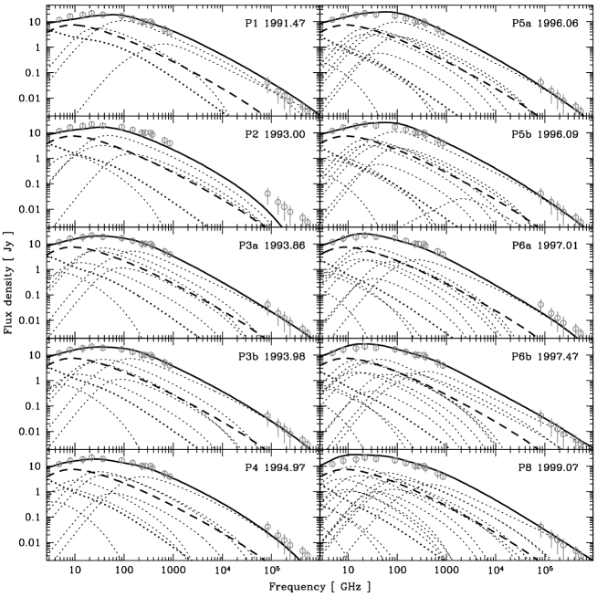
Figure 5: The synchrotron spectra of 3C 279 at 10 EGRET epochs. The points indicate the observed mean flux density levels. The solid line is the total model spectrum at each epoch which is the sum of the spectra of the underlying jet component (dashed line), the overall spectrum of the outbursts peaking before 1989.0 (thick dotted line) and the individual outbursts (dotted lines).

To discuss further the link between gamma-ray emission and synchrotron outbursts we show in Fig. 5 the low-frequency spectral decomposition at each EGRET epoch as derived from our lightcurve fitting. For each epoch, the total model spectrum and its decomposition into individual outbursts is compared to the average spectrum of 3C 279 (points). We see that at two of the high gamma-ray state epochs (P1 and P8) the model spectrum in the optical range is clearly above the average observed flux density levels, but at two other epochs (5a and 5b) the model spectrum fits very well the average optical flux density. At these epochs it is instead the mm/submm flux density which is above the average, which is not seen in epochs P1 and P8. This is easy to understand by looking at the dominant shock components at these epochs: at P1 and P8 the last outburst is high-frequency peaking, while the ninth outburst at epochs 5a and 5b peaks in the millimeter range.

There are four epochs when the fitted optical spectrum is below the observed mean flux density level. Three of these epochs correspond to a low gamma-ray state and the fourth to a moderate gamma-ray flux (epoch P6b). There are also two epochs (P2 and P6a) corresponding to low gamma-ray states and for which the millimeter to submillimeter spectrum is below the observed mean spectral energy distribution. Finally, we note that the centimeter spectrum is dominated by the underlying jet component at all epochs, and that the fitted spectrum is below the observed one at the first two epochs but above it at the last three epochs.

In summary, the pattern we see in Fig. 5 is in accordance with and strengthens the hypothesis that gamma-ray emission originates in young, growing shocks which are dominant in the mm-to-optical regime at the time of high gamma-ray states.

5 Conclusions

We have studied synchrotron flaring in the jet of 3C 279 by decomposing the multifrequency lightcurves into a series of outbursts. The analysis is performed within the generally accepted shock-in-jet scenario, with the evolution of the model outbursts following the Marscher & Gear (1985) prescription. Similar methods have been used previously to study the quasar 3C 273 (Türler et al. 1999, 2000) and the micro-quasar GRS 1915+105. For 3C 279 we find:

1. The lightcurve decomposition supports the Marscher & Gear model. The smooth low-frequency lightcurves are especially well reproduced by the model. In the high-frequency (millimeter to optical) domain, the sharp peaks of the observed lightcurves are less well reproduced by the model lightcurves during the strongest outbursts. Although the model used here makes a lot of assumptions and simplifications which might not hold in detail, it is still clear that there is some mechanism at work which is not well described by the Marscher & Gear (1985) model, and which produces the sharp peaks of outbursts at high frequencies. This is in accordance with previous findings (e.g. Valtaoja et al. 1999): both the theoretical and numerical jet models always produce smooth peaks in model lightcurves while the observed outbursts have exponential rises, sharp peaks and exponential decays.

2. The outburst evolution in 3C 279 follows the characteristic three stage pattern but instead of the synchrotron plateau stage seen in 3C 273, the flux density is already decreasing during the second stage. This might be explained by a highly non-adiabatic jet flow, where radiative losses play a significant role. We also find that the lightcurve of an average outburst is different for 3C 273 and 3C 279. The differences found between these two sources appear to be mainly intrinsic and not due to different orientations. The borderline blazar 3C 273 is thus not simply 3C 279 seen from a larger viewing angle.

3. We find a rather good agreement between the zero-separation epoch of VLBI components and the start times of model outbursts. However, some high-frequency peaking outbursts do not have a corresponding VLBI component which can be explained by the long delay before their spectral turnover reaches VLBI frequencies.

4. When comparing the gamma-ray state at different epochs from Hartman et al. (2001) to the time elapsed since the start of the last synchrotron outburst we find that the shortest time intervals (corresponding to the shortest distances from the apex of the jet to the shock) are seen during the highest gamma-ray states, and the longest ones during the lowest gamma-ray states. This supports previous findings (e.g. Valtaoja & Teräsranta 1996; Jorstad et al. 2001; Lähteenmäki & Valtaoja 2003) that the gamma-ray flares are connected to shocks propagating in the jet. Although during the highest states the shock components are rather new, they are still well outside the outer limits of the broad-line region. This suggests that external Compton models based on the soft-photon field originating from the BLR are unlikely to be able to explain the gamma-ray flares in this source.

- (1) Björnsson, C.-I. &Aslaksen, T., 2000, ApJ, 533, 787
- (2) Gómez, J., 2005, Future Directions in High Resolution Astronomy: The 10th Anniversary of the VLBA, ASP Conference Proceedings, Vol. 340. Edited by J. Romney and M. Reid. San Francisco: Astronomical Society of the Pacific, p.13
- (3) Hanski M., Takalo, L. O., Valtaoja, E. 2002, A&A 394, 17
- (4) Hartman, R. C., et al. 1996, ApJ 461, 698
- (5) Hartman, R. C., Böttcher, M. et al. 2001, ApJ 553, 683
- (6) Hartman, R. C., Villata, M., Balonek, T. J. et al. 2001, ApJ 558, 583
- (7) Impey, C. D., Malkan, M. A.& Tapia, S., 1989, ApJ, 347, 96
- (8) Jorstad, S. G., Marscher, A. P. et al. 2001, ApJ, 556, 738
- (9) Jorstad, S. G., Marscher, A. P. et al. 2004, ApJ, 127, 3115
- (10) Jorstad, S. G., Marscher, A. P., Lister, M. L. et al., 2005, AJ, 130, 1418
- (11) Kaspi, S., Smith, P. S. et al. 2000, ApJ, 533,631
- (12) Katajainen S., Takalo, L. O. et al. 2000, A&AS 143, 357
- (13) Lindfors, E. J., Valtaoja, E.& Türler, M. 2005, A&A, 440, 845
- (14) Lister M. L., Marscher, A. P.& Gear, W. K 1998, ApJ, 504, 702
- (15) Litchfield, S.J., Stevens, J.A., Robson, E.I., Gear, W. K. 1995, MNRAS, 274, 221
- (16) Lähteenmäki, A. & Valtaoja, E., 1999, ApJ, 521, 493
- (17) Lähteenmäki, A. & Valtaoja, E., 2003, ApJ, 590, 92
- (18) Maraschi L., et al. 1994, ApJ, 435, L91
- (19) Marscher, A.P., Gear W.K. 1985, ApJ, 298, 114
- (20) Marscher, A. P., Jorstad, S. G., Mattox, J. R.& Wehrle, A. E. 2002, ApJ, 577, 85
- (21) Reuter, H.-P., Kramer, C. et al. 1997, A&AS, 122, 271
- (22) Robson E.I., Stevens, J.A., Jenness, T. 2001, MNRAS, 327, 751
- (23) Savolainen T., Wiik K. et al. 2002, A&A, 394, 851
- (24) Savolainen T., Wiik, K., Valtaoja, E., Tornikoski, M. 2006, A&A, 446, 71
- (25) Sikora, M., Begelman, M. C., & Rees, M. J. 1994, ApJ, 421, 153
- (26) Steppe, H., Paubert, G. 1993, A&AS, 102, 611
- (27) Stevens, J.A., Litchfield, S.J., Robson, E. I., et al., 1994, ApJ 437, 91
- (28) Stevens, J.A., Litchfield, S.J., Robson, E. I., et al., 1995, MNRAS 275, 1146
- (29) Stevens, J.A., Litchfield, S.J., Robson, E. I., et al., 1996, ApJ 466, 158
- (30) Stevens, J.A., Robson, E. I., Gear, W. K., et al., 1998, ApJ 502, 182
- (31) Teräsranta H., Tornikoski, M. et al. 1998, A&AS 132, 305
- (32) Teräsranta H. et al. 2004, A&A 427, 769
- (33) Tornikoski, M., Valtaoja, E. et al. 1994, A&A 289, 673
- (34) Tornikoski, M., Valtaoja, E. et al. 1996, A&AS 116, 157
- (35) Türler, M., Courvoisier, T.J.-L., Paltani, S. 1999, A&A, 349, 45
- (36) Türler, M., Courvoisier, T.J.-L., Paltani, S. 2000, A&A, 361, 850
- (37) Türler, M., Courvoisier, T.J.-L., Chaty, S., Fuchs, Y. 2004, A&A, 415, L35
- (38) Valtaoja, E., Valtaoja, L., Efimov, Yu. S. & Shakhovskoy, N. M., 1990, AJ, 99, 769
- (39) Valtaoja, E., Teräsranta, H., Urpo, S. et al. 1992, A&A, 254, 71
- (40) Valtaoja, E. & Teräsranta, H. 1996, A&AS, 120, 491
- (41) Valtaoja, E., Lähteenmäki A., Teräsranta, H. & Lainela, M. 1999, ApJS, 120, 95
- (42) Valtaoja, L., Valtaoja, E., Shakhovskoy, N. M., et al. 1991, AJ, 102, 1946
- (43) Villata, M., Raiteri, C. M. et al. 1997, A&AS, 121, 119
- (44) Wehrle, A. E. et al. 2001, ApJS, 133, 297
- (45) Webb, J. R., Carinin M. T. et al. 1990, AJ 100, 1452