Line Strengths in Early-Type Cluster Galaxies at $z$=0.33:Implications for $\alpha$/Fe, Nitrogen and the Histories of E/S0s

Abstract

In this paper we analyze previously published spectra with high signal-to-noise ratios of E and S0 galaxies in the rich cluster CL1358+62 at $z=0.33$, and introduce techniques for fitting stellar population models to the data. These data and methods will be used further in a larger study of the evolution of absorption line strengths in intermediate redshift clusters. Here we focus on the 19 elliptical and lenticular galaxies with an homogeneous set of eight blue Lick/IDS indices. These early-type galaxies follow very narrow line strength-line width relations using Balmer and metal lines, indicating a high degree of uniformity in their formation and enrichment histories. We explore these histories using recently published, six-parameter stellar population models (Thomas, Maraston, & Bender, 2003a; Thomas, Maraston, & Korn, 2004), and describe a novel approach for fitting these models differentially, such that the largest sources of systematic error are avoided. The results of the model fitting are accurate relative measures of the stellar population parameters, with typical formal errors of $\lower 1.29167pt\hbox{$\scriptscriptstyle\;\buildrel<\over{\sim}\;$}0.1$ dex. The best-fit models yield a mean $\chi^{2}$ of 1.2 per degree of freedom, indicating that the models provide good descriptions of the underlying stellar populations. We find: (1) no significant differences between the best-fit stellar population parameters of Es and S0s at fixed velocity dispersion; (2) the stellar populations of the Es and S0s are uniformly old, consistent with results previously published using the fundamental plane; (3) a significant correlation of [Z/H] with galaxy velocity dispersion, in a manner consistent with the observed $B-V$ colors of the galaxies, and indicating that dust is not a significant contributor to the colors of early-type galaxies; (4) a possible, modest anti-correlation of [$\alpha$/Fe] with velocity dispersion, with $<2\sigma$ significance, and discrepant with the correlation inferred from data on nearby galaxies at the $<3\sigma$ level; and (5) a significant anti-correlation of [$\alpha$/N] with galaxy velocity dispersion, which we interpret as a correlation of nitrogen enhancement with mean metallicity. Neither [$\alpha$/C], nor [$\alpha$/Ca] shows significant variation. While the differences between our conclusions and the current view of stellar populations may point to serious deficiencies, our deduced correlation of mean metallicity with velocity dispersion does reproduce the observed colors of the galaxies, as well as the slope of the local Mg-$\sigma$ relation. Our tests indicate that the inferred population trends do describe real galaxies quite well, and matching our results with published data on nearby galaxies, we infer that the discrepancy stems largely from the historical treatment of broadening corrections to the narrow indices. The data also strongly indicate that secondary nitrogen is an important component in the chemistry of elliptical and lenticular galaxies. Taken together, these results reduce early-type galaxies in clusters to a family with one-parameter, velocity dispersion, greatly simplifying scenarios for their formation and evolution. More specifically, our data conclusively show that cluster S0s did not form their stars at significantly later epochs than cluster ellipticals of the same mass, and the presence of secondary nitrogen indicates that both Es and S0s formed from self-enriching progenitors, presumably with extended star-formation histories.

1. Introduction

Ever since the discovery that early-type galaxies follow scaling relations (Morgan & Mayall, 1957), it was clear they had profound implications for cosmology as well as for galactic structure, formation, and evolution (e.g. Minkowski, 1962; Terlevich et al., 1981, and subsequent literature). Perhaps the most well-studied of these scaling relations is the color-magnitude relation (Baum, 1959), and its interpretation as a correlation of metal abundance with galaxy luminosity (Rood, 1969) has survived to the present-day. Over the past several decades, numerous other scaling relations have been discovered and interpreted, such as $L$-$\sigma$ (Faber & Jackson, 1976), $r_{e}$-$I_{e}$-$\sigma$ (the fundamental plane; Dressler et al., 1987; Djorgovski & Davis, 1987), Mg-$\sigma$ (Terlevich et al., 1981), and other line strength-line width relations, such as H$\delta_{A}$- or H$\gamma_{A}$-$\sigma$ (e.g. Kuntschner, 2000; Kelson et al., 2001).

Several important breakthroughs have helped to constrain the nature of early-type galaxy scaling relations. The clearest results have come from explicit tests for changes in the ages of stellar population with redshift along the sequence of early-types. By measuring the slopes of the color-magnitude relations in clusters to redshifts of unity Stanford, Eisenhardt, & Dickinson (1998) concluded that the relation originates largely from systematic variations in metallicity with galaxy mass (also see Blakeslee et al., 2006). Likewise, the fundamental plane of early-type galaxies has a slope that does not appear to evolve significantly with redshift to $z=0.33$ (Kelson et al., 2000c), further evidence that cluster E/S0s are a family well-described by uniform ages and a mass-metallicity relation. At redshifts of $z=0.8-0.9$ there are hints that the slope of the fundamental plane may evolve modestly (Jørgensen et al., 2006), though this result appears to be inconsistent with the slope of the color-magnitude relation as measured by Blakeslee et al. (2006) and it remains to be seen how these data will be reconciled.

There have been many efforts to observe the high-redshift line strength-line width relations (Ziegler & Bender, 1997; Kelson et al., 2001; Jørgensen et al., 2005; Barr et al., 2005; Moran et al., 2005). However, significant constraints have not been forthcoming because of the difficulty of obtaining sufficient signal-to-noise ratios.

The situation is much better at low redshifts. Detailed analysis of line strengths in low-redshift E/S0s have been very revealing since González (1993) (and others) broke the age-metallicity degeneracy (Worthey, 1994). Using line strengths many authors have shown that massive galaxies in clusters are uniformly old (e.g. Jørgensen, 1997, 1999; Trager et al., 2000a; Kuntschner, 2000), but some ambiguities do remain. For example it has long been understood that the Mg$b$-$\sigma$ (Terlevich et al., 1981) and Fe-$\sigma$ (González, 1993) relations are not consistent with the hypothesis that they both arise solely from a correlation between the mean metallicity of the stellar populations and galaxy mass. The discrepancy has been interpreted using stellar populations models in which “$\alpha$-enhancement, or [$\alpha$/Fe], is allowed to vary systematically with velocity dispersion (see, e.g. Jørgensen, 1999; Trager et al., 2000a, b; Worthey & Collobert, 2003; Thomas et al., 2005, for details and many important references). While Trager et al. (2000a) reminded readers that this is a misnomer, because the $\alpha$ elements are not enhanced — Fe is simply under-abundant. We will, however, continue to use the term “$\alpha$-enhancement” to be consistent with past literature on the subject. After several decades of analysis, improved techniques of observation, and despite the immense amount of progress in stellar population models (Faber, 1972; Worthey, 1994; Trager et al., 2000a; Schiavon et al., 2002; Thomas, Maraston, & Bender, 2003a), the modeling of absorption lines remains ambiguous and contradictory (e.g., Worthey, 1994; Trager et al., 2000b; Worthey & Collobert, 2003; Schiavon, Caldwell, & Rose, 2004; Thomas, Maraston, & Bender, 2003b, and others). Some have even questioned the “$\alpha$-enhancements” altogether (Proctor et al., 2004a).

Over the long-term we hope that the physics of stellar atmospheres will be understood with sufficient detail to allow for the creation of synthetic stellar spectra for stars, over the full range of stellar masses and phases of stellar evolution, that comprise the observed spectra of galaxies. Presently, however, numerous uncertainties in the formation of molecular lines, and incomplete line lists prevent one from generating completely synthetic spectra for stellar populations. As a result the features in the spectra of stars and galaxies cannot be fully modeled. Despite major progress in generating high resolution spectral energy distributions of simple stellar populations (Vazdekis, 1999; Bruzual & Charlot, 2003), we cannot fully solve for the age(s) and elemental abundances of populations in a galaxy by directly fitting synthetic spectra.

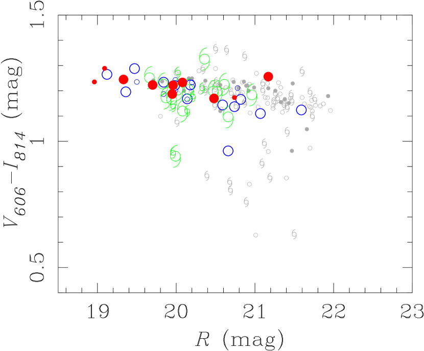
Figure 1.— Color-magnitude diagram of the cluster in $R$ and $V_{606}-I_{814}$, taken from Kelson et al. (2000b). All 194 confirmed cluster members in the HST imaging are shown. The red, blue, and green symbols represent those galaxies observed by Kelson et al. (2000b) for use in their study of the fundamental plane. Ellipticals are shown using red, filled circles. The S0 galaxies are shown using blue open circles. Spiral galaxies are shown in green. The light gray points were not observed in the high-resolution study of Kelson et al. (2000b). The red, blue, and green points are shown using two sizes. The larger ones mark those galaxies in the homogeneous sample (for which all eight of the indices used in the modeling are available; see §3). The E and S0 (red and blue) galaxies in the figure are discussed in this paper while the full fundamental plane sample of CL1358+62 will be discussed in a subsequent paper.

Without the ability to directly model the spectra of galaxies, one must measure and model spectral indices. One widely used system is the Lick/IDS system, created by Burstein et al. (1984) (and subsequently revised by Trager et al., 1998). To this day, the measurement and modeling of these line strengths remain the most useful means of assessing the bulk properties of the stellar populations in passively evolving galaxies.

Over the last several years several groups have expanded our ability to model these indices with more parameters than age, metallicity, and $\alpha$-enhancement. The models of Trager et al. (2000a),Thomas, Maraston, & Bender (2003a), and Schiavon (2005) allow one to probe specific elemental abundances, such as nitrogen, carbon, and calcium. Such models only make predictions for passively evolving stellar populations. Fortunately models of galaxy evolution involving star-formation are not needed in our study of massive cluster galaxies through intermediate redshifts, because such galaxies have been shown to be passively evolving (e.g., Kelson et al., 1997, 2000c; Wuyts et al., 2004). At higher redshifts, on-going star-formation may become increasingly important (e.g. Juneau et al., 2005), and more sophisticated models may then be required.

In our survey of galaxies in rich clusters at intermediate redshifts, the sample of galaxies with the highest signal-to-noise spectroscopy over the widest range of galaxy luminosities is that from our fundamental plane survey of CL1358+62 at $z=0.33$. Because of the depth and quality of that sample, we adopt it as the reference sample to which the other clusters in our survey will subsequently be compared (Kelson et al., 2006b).

Here we study the absorption lines of the E/S0 galaxies in that sample, using the models of Thomas, Maraston, & Bender (2003a) and Thomas, Maraston, & Korn (2004) to explore not only ages and metallicities, but additional stellar population parameters, namely the relative abundances of nitrogen, carbon, and calcium, along with the mean $\alpha$-enhancement. Because we are keenly interested in potential variations in the abundance ratios, and because the state-of-the art high-resolution models (Bruzual & Charlot, 2003) do not reproduce, in detail, the strengths of many features in the spectra of real galaxies (e.g. CN, Ca4227, Mg, H$\delta$, H$\gamma$; Gallazzi et al., 2005), we prefer to derive stellar population parameters from an analysis of absorption line indices. The Bruzual & Charlot (2003) SEDs are employed for other purposes and these are discussed below in the context of deriving broadening corrections to our data.

Many of the details regarding the processing of the data, and subsequent corrections, are discussed elsewhere (Kelson et al., 2000b, 2006a). However several of the key points are discussed below in §2 because of their crucial role in the analysis. We then describe our comparison of the absorption line strengths of the E/S0 galaxies to the models of Thomas, Maraston, & Bender (2003a) and Thomas, Maraston, & Korn (2004), in which we perform non-linear least-squares fits to each galaxy’s set of line strengths (see, also Proctor et al., 2004), but only for relative differences in the stellar population parameters. This allows us to explicitly avoid potentially large systematic uncertainties in the direct comparison of the data and models. This methodology is used in the rest of the survey and so is described in some detail. The resulting relative ages and patterns of fitted chemical abundances are described in §4 and then discussed further in §5. Our conclusions are summarized in §6. While our findings do not depend on the cosmology, we use the cosmological parameters $H0=72$ km/s/Mpc, $\Omega_{M}=0.27$, and $\Omega_{\Lambda}=0.73$, when such parameters are required (e.g. for corrections to the line strengths for any variation in the metric sizes of the apertures from which the spectra were obtained).

2. The Data

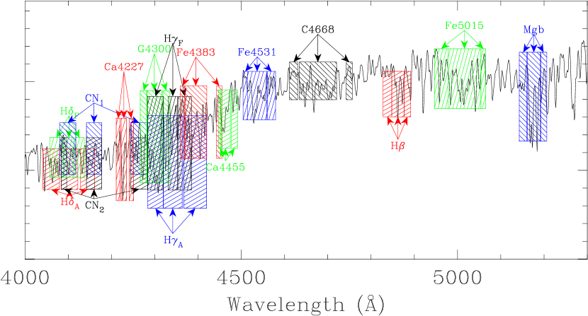
Figure 2.— Overlayed on a model spectrum of a 6 Gyr-old population (Bruzual & Charlot, 2003) is the set of Lick/IDS bandpasses used in this paper (Worthey et al., 1994; Trager et al., 1998)

As stated earlier, the galaxies in CL1358+62 were originally targeted as part of a survey to study the fundamental plane in intermediate redshift clusters (published by Kelson et al., 1997; van Dokkum et al., 1998b; Kelson et al., 2000c; Wuyts et al., 2004). The selection of the CL1358+62 spectroscopic sample, and data processing, were fully described in Kelson et al. (2000b), and we summarize it here.

The field of CL1358+62 was targeted for extensive imaging with the HST WFPC2. A two-color mosaic of the cluster CL1358+62 covering $64\,{\mathchoice{\vbox{\vbox{\hrule height=0.2pt\hbox{\vrule width=0.2pt,height=6.0pt\kern 6.0pt\vrule width=0.2pt} \hrule height=0.2pt}}}{\vbox{\vbox{\hrule height=0.2pt\hbox{\vrule width=0.2pt,height=6.0pt\kern 6.0pt\vrule width=0.2pt} \hrule height=0.2pt}}}{\vbox{\vbox{\hrule height=0.1pt\hbox{\vrule width=0.1pt,height=4.2pt\kern 4.2pt\vrule width=0.1pt} \hrule height=0.1pt}}}{\vbox{\vbox{\hrule height=0.1pt\hbox{\vrule width=0.1pt,height=3.0pt\kern 3.0pt\vrule width=0.1pt} \hrule height=0.1pt}}}}\,\,^{\prime}$ was constructed using 12 pointings. Of the spectroscopically confirmed members (Fisher et al., 1998), 194 fall within the field of view of the WFPC2 imaging. From this large catalog, we selected a sample for detailed study with the Low Resolution Imaging Spectrograph (LRIS; Oke et al., 1995) at the W.M. Keck Observatory. The high resolution of the HST imaging allowed us to derive structural parameters with the accuracy needed for the fundamental plane (Kelson et al., 2000a, c).

The sample used in the fundamental plane analysis was randomly selected from a catalog of known members within the field of the HST mosaic down to $R<21$ mag. Because the selection did not rely on morphological information, the galaxies span a range of morphologies, from ellipticals to spirals. In Figure 1, taken from Kelson et al. (2000b), we show the color-magnitude diagram for the spectroscopically confirmed cluster members within the HST mosaic. At the redshift of the cluster, $L^{*}$ corresponds to $R\sim 20.1$ mag (adopting the $M/L_{V}$ evolution as measured by Kelson et al., 2000c). There is clearly a tight color-magnitude relation in the cluster, fully analyzed in van Dokkum et al. (1998a). The entire catalog of spectroscopically confirmed cluster members within the HST mosaic is shown by the circles, and those selected for fundamental plane analysis are shown by the filled circles. As can be seen in the figure, the sample fairly represents the cluster population, minus the faint (and very blue) objects.

In Fisher et al. (1998) there are 108 members brighter than $R=21$ mag within the HST mosaic. Our high-resolution spectroscopic sample contains 52 of them. Three cluster galaxies fainter than the magnitude limit were added, bringing the total number of the sample to 55. The spectra were shown in Kelson et al. (2000b), and the signal-to-noise ratios ranged from about 15 per Å to 90 per Å. The 900/mm grating provided a typical resolution of $\sigma_{inst}\approx 60$ km/s. Details of the reductions to one-dimensional spectra were also given in Kelson et al. (2000b).

Below we describe the methods for measuring the absorption line strengths and velocity dispersions. The algorithm for deriving the latter is necessary because we employ portions of it in determining the corrections for Doppler and instrumental broadening, and for estimating the formal uncertainties in the line strengths. Fuller discussions of our measurements of the absorption line strengths, including the procedures to estimate formal errors, the procedures to correct the line strengths for the Doppler and instrumental broadenings, and the corrections for the different metric aperture sizes are contained in Kelson et al. (2006a).

2.1. Absorption Line Strengths

At this time the best understood and modeled diagnostics remain the spectral indices of the Lick/IDS system (Faber et al., 1985; Burstein et al., 1984; Burstein, Faber, & Gonzalez, 1986; Gorgas et al., 1993; Worthey et al., 1994), defined as a set of indices measuring the strengths of Balmer, metal, and molecular features. We adopted the Trager et al. (1998) definitions for the Lick/IDS indices, with the additional definitions of Worthey & Ottaviani (1997) for the indices of the higher order Balmer lines H$\delta$ and H$\gamma$. Each index is comprised of a blue continuum bandpass, a central index bandpass, and a red continuum bandpass.

The bandpasses of the blue indices are shown graphically in Figure 2. Note that the stellar absorption lines covered by each index are heavily blended in galaxy spectra as a result of Doppler broadening and smoothed further by the line-spread function of the instrument. In order to compare line indices from one galaxy to another, or from data taken with one instrumental set-up to data taken with another, the indices must be corrected to identical levels of intrinsic Doppler and instrumental broadenings, and these corrections are discussed below.

The absorption line strengths were measured using the following prescription:

The straight line between the mean fluxes in the two continuum bandpasses is defined as the local continuum, $C_{\lambda}$, within the index bandpass. The mean flux within a bandpass is written as:

$$F_{p}={1\over(\lambda_{2}-\lambda_{1})}\int_{\lambda_{1}}^{\lambda_{2}}F_{\lambda}d\lambda$$ (1)

Each index is then defined by the integral of the residual flux above and/or below the local continuum within the index bandpass (Worthey, 1994). For convenience we define

$$I_{p}={1\over(\lambda_{2}-\lambda_{1})}\int_{\lambda_{1}}^{\lambda_{2}}{F_{\lambda}\over C_{\lambda}}d\lambda$$ (2)

The metal and Balmer line strengths have units of Å and are commonly referred to as pseudo-equivalent widths, while molecular features are expressed as magnitudes:

$$X_{\rm ew} = \bigl{(}{\lambda_{2}-\lambda_{1}}\bigr{)}(1-I_{p})$$ (3)

$$X_{\rm mag} = -2.5\log I_{p}$$ (4)

The integrations are straightforward, with the contributions from partial pixels computed using linear interpolation.

2.2. Velocity Dispersions

Many scaling relations of early-type galaxies use galaxy velocity dispersion, $\sigma$, as the dependent variable (e.g. Faber & Jackson, 1976; Terlevich et al., 1981; Djorgovski & Davis, 1987; Dressler et al., 1987). Reliable measurement of velocity dispersion is also key to deriving reliable line strengths as the velocity dispersions are required to compute the Doppler corrections to the line strengths. The procedures used for deriving $\sigma$ are also used in our method to estimate the formal errors in the line strengths.

Our preferred method for measuring velocity dispersions is the direct-fitting method (described by Kelson et al., 2000b, though also see (Rix & White, 1992)), It has several advantages over techniques that operate in Fourier space (e.g. Tonry & Davis, 1979; Franx, Illingworth, & Heckman, 1989). Most importantly, when measuring velocity dispersions of high-redshift galaxies, non-uniform sources of noise become important, and these affected pixels should not be accorded uniform weight. By fitting spectra directly, one measures the velocity dispersion by shifting and broadening a template spectrum until the result matches each galaxy spectrum (Burbidge, Burbidge, & Fish, 1961; Rix & White, 1992). Mathematically, one has a galaxy spectrum, $G$, and a template spectrum, $T$, and one searches for the line-of-sight velocity distribution $B$, that is used to convolve $T$ such that $\chi^{2}$ is minimized: (Kelson et al., 2000b):

$$\chi^{2}=\bigl{|}\bigl{\{}G-\bigl{[}P_{M}(B(\sigma,v)\circ T)+\sum_{j=0}^{K}a_{j}H_{j}\bigr{]}\bigr{\}}\times W\bigr{|}^{2}.$$ (5)

Following Kelson et al. (2000b) we parameterize the line-of-sight velocity distribution as a Gaussian, $B(\sigma,v)$, in which $\sigma$ is the velocity dispersion, or second moment of the velocity distribution and, $v$ is the mean radial velocity, or first moment of the velocity distribution. The fit also includes two additional components: $P_{M}$, a low-order multiplicative polynomial that incorporates the difference between the instrumental response function in $G$ and $T$, and $\sum a_{j}H_{j}$ is an additive continuum function comprised of sines and cosines up to wavenumber $K$ (Kelson et al., 2000b). These sines and cosine continuum functions are equivalent to filtering low wavenumbers in the Fourier domain (see, e.g., Tonry & Davis, 1979).

The unique value of the direct-fitting method is contained in $W$, the weighting spectrum. We opt, as in Kelson et al. (2000b), to weight most pixels by the inverse of the noise, estimated from photon statistics and amplifier read noise. Just as in Kelson et al. (2000b), there are exceptions: (a) regions contaminated by galactic emission lines are given zero weight; (b) strong Balmer absorption lines are also given zero weight; and (c) pixels contaminated by poorly subtracted night-sky emission lines are also given zero weight. Nearly all of the early-type galaxies discussed in this paper have no (or very weak) emission. The BCG, however, does have emission lines and therefore it is the only galaxy in this paper for which this “masking” is important. The fitting was performed between $\sim 4250$Å and $\sim 5050$Å, in the rest-frame, employed 5th-order for the multiplicative polynomial, $P_{M}$, and sines and cosines up to $K=6$. The results, as shown by Kelson et al. (2000b), are sensitive to these choices only at the level of a few percent.

The template spectra spanned a range of late-type stars, as was also discussed previously in Kelson et al. (2000b). Ideally one might wish to employ spectra which represent more accurate models of the galaxy spectra. However, the current state-of-the-art high-resolution model spectra (Bruzual & Charlot, 2003) have lower resolution ($\sim 3$Å) than our instrumental setup ($\sim 1.7$Å). Therefore these model spectra are not suitable for providing accurate measurements of velocity dispersion in our lower-mass galaxies. If one derives velocity dispersions using the Bruzual & Charlot (2003) SEDs, the one must add, in quadrature, the difference in resolution to the result. Doing so, we find $<1\%$ systematic difference between those sigmas and the ones we obtained using the Kelson et al. (2000b) stellar templates, with a standard deviation of 2%. Furthermore, there is no statistically significant trend with velocity dispersion for galaxies with $\sigma>100$ km/s.

2.3. Absorption Line Strength Errors

Accurate estimates of the uncertainties in absorption line strengths require one to determine the variances within each index bandpass (e.g., González, 1993; Cardiel et al., 1998). One can adopt the expected noise due to photon statistics and amplifier read noise, but sources of noise become increasingly localized for high redshift galaxy spectra, with the bright OH lines and, potentially, fringing dominating the errors in flux. Furthermore, the noise can become correlated in adjacent pixels after the data are rebinned onto a simple wavelength scale (Cardiel et al., 1998).

We developed an approach that provides for a more robust determination of the line strengths and their errors, with less susceptibility to systematic errors. This approach requires neither the additional overhead of variance images nor any assessment of correlated noise in adjacent pixels. Furthermore, our method does not rely on the assumption that the “true” noise is well-represented by the theoretical expectation from photon statistics and the electronics noise. Tests with the data and simulations indicate that our methodology produces accurate estimates of line strength errors. We discuss the method here.

Deriving the random errors in absorption line strengths requires knowledge of the total variances in the continuum and index bandpasses. Given an observed galaxy spectrum $G$, the noise in a given pixel is simply $N=G-R$, where $R$ represents the underlying, noiseless spectrum of the galaxy. While there is no a priori knowledge of $R$, Equation 5 allows us to write

$$R\approx\widetilde{R}=P_{M}(B\circ T)+\sum_{j=0}^{K}a_{j}H_{j}$$ (6)

Using the model stellar population spectra of Bruzual & Charlot (2003), we generated the best-fit model SED for each galaxy. The model spectra were used, instead of our template stars, because they better reproduce the Balmer, metal, and molecular line strengths in $G$. One should note, however, that in searching for the best-fit SED, no unique best-fit age/metallicity pair could be found for any given galaxy: young, metal-rich model SEDs fit as well as old, metal-poor model SEDs in all cases, with complete degeneracy. Because individual line strengths are subject to a similar degeneracy between age and metallicity (e.g., Worthey, 1994), attempts to match the detailed spectra are subject to the mean correlation between age and metallicity because the computation of $\chi^{2}$ utilizes all of the spectral features simultaneously.

The approximation to $R$ provides an approximation to $N\approx\widetilde{N}$.

$$\widetilde{N}=G-\bigl{[}P_{M}(B\circ T)+\sum_{j=0}^{K}a_{j}H_{j}\bigr{]}$$ (7)

With $\widetilde{N}$ the variance in the mean flux, $F_{p}$, is

$$V_{F_{p}}={1\over{\lambda_{2}-\lambda_{1}}}\sum_{i}^{n}{\widetilde{N}_{i}}^{2}\Delta\lambda_{i}$$ (8)

where the summation is over the pixels within the given bandpass and $n$ is the number of pixels within the bandpass. For pixels of constant $\Delta\lambda$, this reduces to the familiar

$$V_{F_{p}}={1\over n}\sum_{i}^{n}{\widetilde{N}_{i}}^{2}$$ (9)

where the error in the mean flux is then

$$\varepsilon_{F_{p}}=\sqrt{{1\over n^{2}}\sum_{i}^{n}{\widetilde{N}_{i}}^{2}}$$ (10)

Note that partial pixels are included at the ends of the bandpass by linearly interpolating the fractional contribution of that pixel to the bandpass and adding those to the summation. For clarity we did not include them in the above equations.

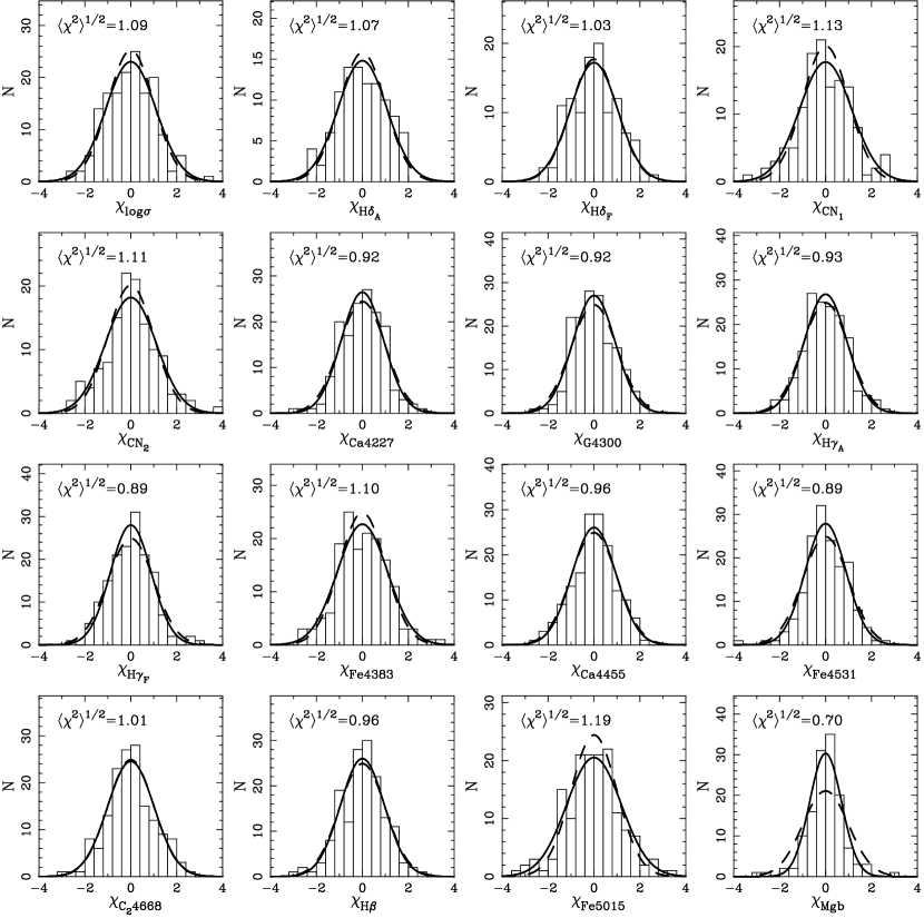
Figure 3.— Histograms showing the variance in the measurements of the indices from the individual exposures. Each galaxy’s spectrum was observed in three exposures and a comparison between the line strengths in the individual exposures provides an independent test of our estimates for the formal errors. The dashed curves show Gaussians with standard deviations of unity to illustrate the expected distribution of the data. The solid curves show Gaussians with standard deviations determined empirically and listed within each panel. Excluding Mg$b$, the mean standard deviation is 0.95, indicating that the formal errors in our line strengths have been properly estimated. The Mg$b$ bandpass suffers from telluric absorption and our correction to it is uncertain. As a result the residual telluric absorption reduces the variance between the individual observations.

With accurate estimates of the errors in the mean flux of each bandpasses the total uncertainties in the line strengths can be trivially computed by propagating the errors in a manner mathematically equivalent to González (1993). The key to our method is that the determination of the variances in each bandpass do not rely on simple photon statistics. In detail, the models may not provide perfect matches within the line strength bandpasses but these detailed departures from the models only become important when template-mismatch dominates the errors in the velocity dispersion fitting. In the original reference for these spectra (Kelson et al., 2000b), template-mismatch appears to become significant beyond $S/N>60$ per Å, but does not dominate the residuals between a galaxy spectrum and the model fit to it until one has significantly higher S/N ratios. Furthermore, by including functions in the fit for matching the continuum, broad mismatches are improved, such as for CN or C4668.

The accuracy of our error estimates was confirmed in two ways. First, we performed Monte Carlo simulations, in which we degraded model spectra to a range of $S/N$ ratios and remeasured the absorption line strengths. We found excellent agreement between our error estimates and the scatter in the measured line strengths about the input measurements.

The second approach we took to verify the validity of our error estimates involved exploiting the fact that each spectrum had originally been observed with three exposures. For each exposure we measured the indices and their formal errors and created histograms of the distributions of the indices about their weighted means. These are shown in Figure 3. In the figure, Gaussians with standard deviations of unity (the dashed lines) show the distributions one expects if our formal error estimates are consistent with the differences between the three separate observations per galaxy. The solid lines show Gaussians whose standard deviations are given in each panel and were determined empirically from the observed distribution of line strengths from the individual exposures. Excluding Mg$b$, the mean standard deviation of the histograms is 0.95, indicating that our errors, on average, are over-estimates by approximately 5%. Unfortunately, Mg$b$ is contaminated by telluric absorption at this redshift and our corrections to it are uncertain. Thus for that index the variance between the measurements appears to be systematically reduced, and, we infer, leads to an artificial reduction in $\langle\chi^{2}\rangle$ for its histogram (also see Kelson et al., 2006a, for examples of the spectra). Taken together, these tests indicate that our method for estimating the random errors in the absorption line strengths is accurate for spectra spanning the range of signal-to-noise ratios of these data.

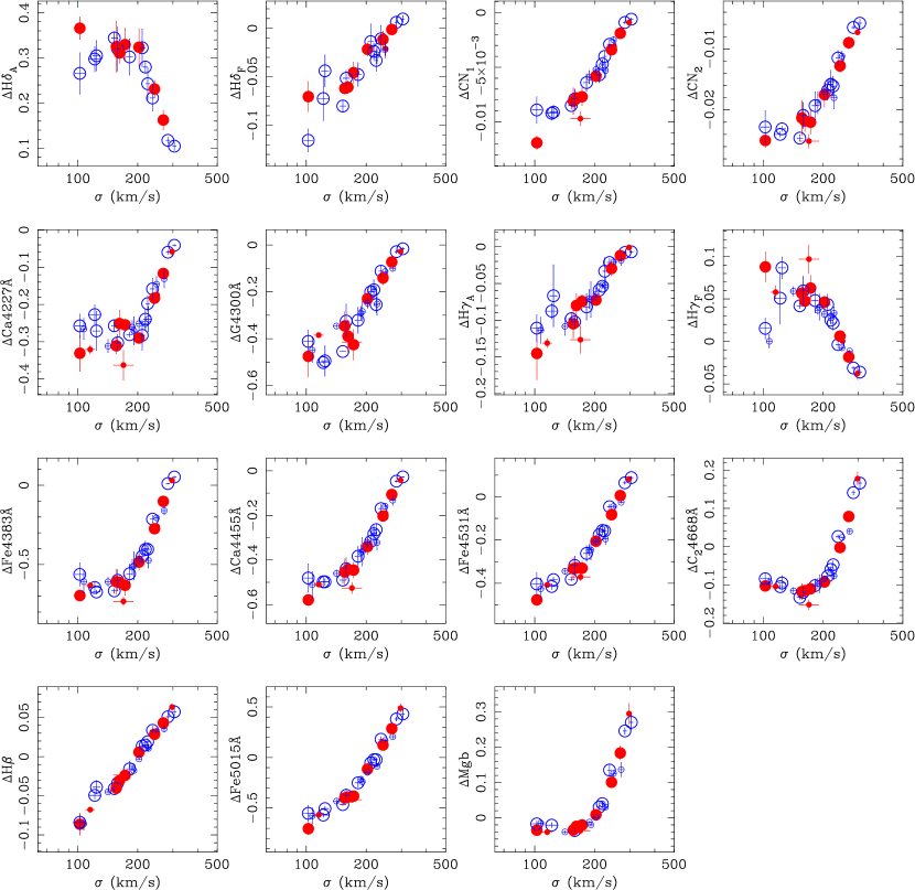
Figure 4.— Broadening corrections to the blue Lick indices for the E/S0s in CL1358+62 as a function of velocity dispersion. Symbols are as in Fig. 1. The increased scatter at low velocity dispersions arises because of an increase in the scatter of the ages and/or metallicities of the Bruzual & Charlot (2003) SEDs used to derive the corrections for each of the galaxies. Much of this increased scatter is not statistically significant, though the variations in the intrinsic strengths of the features, i.e. variations in the underlying SEDs, are important for indices such as H$\gamma_{F}$.

2.4. Correction for Instrumental and Doppler Broadening

In spectra of galaxies, the blending of the absorption lines significantly alters the continuum, and spectra with different intrinsic Doppler or instrumental broadenings will yield different pseudo-equivalent widths. Consequently, measurements of absorption line strengths must be corrected for both the internal motions of the stars and for the finite resolution of the spectrograph. While the system of line strengths could have been defined by spectra with arbitrary levels of intrinsic Doppler or instrumental broadening, the Lick/IDS system of indices is referenced to stars (i.e., spectra with zero Doppler broadening) observed through the IDS, for which the instrumental resolution was characterized in Worthey & Ottaviani (1997). It is important to note that this characterization of the IDS’s instrumental resolution has a very strong dependence on wavelength.

The broadening corrections were computed by measuring an index, $X$, three times for each galaxy: (1) $X|_{G}$, the index measured directly from the galaxy spectrum; (2) $X|_{B(\sigma)\circ T}$, the index measured from the template spectrum (or model SED; see previous section) broadened to the velocity dispersion of the galaxy and at the resolution of the galaxy’s spectrum; and (3) $X|_{T_{IDS}}$, the index measured from the template spectrum (or model SED) with a velocity dispersion of zero and convolved to the resolution of the Lick/IDS system (Worthey & Ottaviani, 1997). Thus, each galaxy’s corrected line strength $X_{cor}|_{G}$ can be recovered by

$$X_{cor}|_{G}=X|_{G}+\biggl{[}X|_{T_{IDS}}-X|_{B(\sigma)\circ T}\biggr{]}$$ (11)

There are two advantages to defining the broadening corrections in this way. First, smoothing the galaxy spectra to low spectral resolution dramatically, and non-trivially alters the statistics because of non-uniform sources of noise. Second, our definition of the broadening corrections allows for sign reversals that can occur as the pseudo-continua change with large differences in Doppler and instrumental broadening. In these cases, such as for the high-order Balmer lines, multiplicative corrections (e.g., González, 1993; Trager et al., 1998) can be problematic.

Because broadening corrections can be sensitive to the adopted template SED, we adopt the best-fit Bruzual & Charlot (2003) SED for $T$. By doing so the systematic error in the broadening corrections is minimized. However, the ages and metallicities of the best-fit Bruzual & Charlot (2003) SEDs are sensitive to the wavelength range of the fit. Therefore we derive broadening corrections using parameters derived from fitting over $\rm 4100\AA\ <\lambda<5000\AA$, $\rm 4200\AA\ <\lambda<4800\AA$, $\rm 4070\AA\ <\lambda<4800\AA$, and $\rm 4070\AA\ <\lambda<4500\AA$, in the restframe. We adopt the mean broadening correction from these four fits, and we use the scatter in their broadening corrections as estimates of the random errors in the corrections.

Fortunately, the large uncertainties in the SED ages ($\sim 0.15$ dex) and metallicities ($\sim 0.3$ dex) are strongly (anti)correlated such that the uncertainties in the broadening correction are small. For all of the indices, the errors in the broadening corrections are estimated to be at a typical level of $\pm 10\%$ of the correction itself; i.e., quite small. More importantly, the uncertainties in the corrections are typically $<3\%$ of the dynamic ranges of the line strengths, as estimated using the 68% widths of the distributions of the indices.

Our broadening corrections are plotted against galaxy velocity dispersion in Figure 4. At velocity dispersions $\sigma\lower 1.29167pt\hbox{$\scriptscriptstyle\;\buildrel<\over{\sim}\;$}150$ km/s, there is an increase in the scatter in the broadening corrections for several indices. Even though these increases in the scatter arise because of an increase in the scatter of the best-fit ages and/or metallicities of the Bruzual & Charlot (2003) SEDs, the increased scatter in the corrections is typically not statistically significant, given the uncertainties in the corrections themselves. A small number of galaxies fall off the primary loci of points for the narrow Balmer indices H$\delta_{F}$ and H$\gamma_{F}$. These galaxies, below the magnitude limit of the sample, do have larger values of these indices, though the wider H$\delta_{A}$ and H$\gamma_{A}$ indices, which will be used in our analysis below, do not show such large departures.

2.5. Correction for Aperture Size

In order to accurately compare samples of galaxies at different redshifts, one must be correct for the effects of observing the galaxies with different aperture sizes. Because this sample will be the reference dataset in our survey of distant clusters Kelson et al. (2006b), we correct the observed line strengths to an effective aperture consistent with the aperture used in the most distant cluster in our sample, MS1054–03, at $z$=0.83. In Kelson et al. (2006a) we detail our formalism for estimating the relationship between the internal line strength gradients in distant galaxies and the dependence of line strength measurements on aperture size.

Using estimates of the line strength gradients for the CL1358+62 sample galaxies, and the relationship between gradient, $\beta$, and aperture correction, $\Delta X$, derived in Kelson et al. (2006a), we have corrected the line strengths of the CL1358+62 galaxies to an aperture equivalent to a diameter $D_{\rm ref}=10.1$ kpc at the distance of MS1054–03 ($D_{ap}=1\hbox{${}^{\prime\prime}$\hbox to0.0pt{\hss.}}35$, using, again, $H0=72$ km/s/Mpc, $\Omega_{M}=0.27$, and $\Omega_{\Lambda}=0.73$). The corrections are defined to be $\Delta X=\beta\times f(D_{ap}/D_{\rm ref})$, where we derived $f(D_{ap}/D_{\rm ref})=0.075$ in Kelson et al. (2006a). The corrections for aperture size are small because the extraction aperture for the CL1358+62 galaxies was chosen to minimize the corrections. As a result, the errors in correcting the aperture to an equivalent aperture at the distance of MS1054–03 are small ($\hbox{${}_{<}\atop{{}^{\sim}}$}10\%$ of the correction).

The uncorrected line strengths for the full sample of galaxies in CL1358+62, are given in several tables of Kelson et al. (2006a). The line strengths of the elliptical and lenticular galaxies, corrected for both broadening and aperture size, are reproduced here in Tables 1 and 2. Though these are the data to be used in the discussions of the stellar populations below, these corrections do not affect the conclusions drawn in this paper.

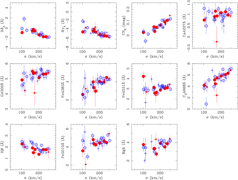
Figure 5.— The line strength-line width relations for E/S0s in the CL1358+62 sample of Kelson et al. (2000c). Ellipticals are shown as filled red circles and E/S0 and S0 galaxies as open blue circles. Note that the measurements of Mg$b$, not used in the fitting for the stellar population parameters, suffer from additional uncertainties arising from poor correction to telluric absorption. The small symbols represent those galaxies that are missing any of the eight required indices for the fitting, and as such belong to a larger inhomogeneous sample. The larger symbols show those galaxies which have all eight indices to be used in the stellar population fitting.

2.6. The Line Strength-Line Width Relations

The correlations between absorption line strengths and velocity dispersion has become a diagnostic for directly probing galaxy evolution (e.g. Ziegler & Bender, 1997; Kelson et al., 2001; Jørgensen et al., 2005). The strengths of the metal, molecular, and Balmer absorption features all correlate with velocity dispersion, and the full multi-dimensional locus of early-type galaxies in the space of velocity dispersion and line strengths has implications for scenarios of their formation, e.g., such as the timescale for the build-up of stellar mass. For example, the (H$\gamma_{A}$+H$\delta_{A}$)-$\sigma$ relation was studied to $z=0.83$ by Kelson et al. (2001) in an effort to directly trace the evolution of the high-order Balmer lines, at fixed velocity dispersion, with redshift.

Before proceeding to detailed modeling of the indices, we show the observed line strength-line width relations for the early-type galaxies in CL1358+62 in Figure 5. Note that the E and S0 galaxies follow statistically identical line strength-line width relations. This fact has consequences for the uniformity of their formation and enrichment histories, and we discuss this further below using simple models.

3. Fitting for the Relative Stellar Population Parameters

The models published in Thomas, Maraston, & Bender (2003a) and Thomas, Maraston, & Korn (2004) contain predictions for the Lick/IDS indices at locations in sparsely sampled “grid” of the six parameters: $\log t$, [Z/H], [$\alpha$/Fe] (mean $\alpha$ enhancement), [$\alpha$/N] (nitrogen enhancement or depletion on top of any enhancement of N as an $\alpha$ element), [$\alpha$/C] (same as [$\alpha$/N] but for carbon), and [$\alpha$/Ca] (for calcium). For clarity, when nitrogen is enhanced with respect to the ensemble of $\alpha$ elements, [$\alpha$/N] decreases. As a reminder, most published results on $\alpha$-enhancement stem from the measurement of indices sensitive to Mg. However, oxygen is the most abundant $\alpha$ element and will likely dominate the $\alpha$ sensitivity in the blue owing to the equilibrium between carbon, nitrogen, and oxygen.

The dependence of these spectral indices on the controlling parameters is non-linear and the inversion of observables to find the luminosity-weighted mean properties of stellar populations is non-trivial. In this section we detail the steps by which we determine the stellar population model parameters that best fit the observed line strengths.

Each of our galaxies in CL1358+62 has between eight and ten indices measured from its spectrum. For every galaxy, we wish to use all of the available data to constrain its star-formation and nucleosynthetic history, as described by the “simple” models. In principle our fit of a simple stellar population (SSP) to a given galaxy has up to six unknowns, and of order ten observables, suggesting that the process of inverting the observables should be straightforward. However, each Lick index measures the combined strength of many blended features in the spectrum of the underlying, unbroadened stellar population. These features are all sensitive to the ages, mean metallicities, and detailed abundance ratios of the stars (Burstein et al., 1984; Worthey et al., 1994; Worthey, 1994; Trager et al., 2000b; Cardiel et al., 2003; Thomas, Maraston, & Bender, 2003a; Thomas, Maraston, & Korn, 2004). To help illustrate these degeneracies, Table 3 lists the first partial derivatives of the model predictions (at a specific reference point, discussed below). These derivatives indicate that the process of fitting models to observed indices will lead to significant covariances between the fitted parameters. The derivatives given in the table are only valid at a single location in the six dimensional space of SSP parameters and the full dependencies of the model predictions on the SSP parameters is nonlinear. Below we describe how the nonlinearity of the models has been treated.

At this time we note that some derivatives are not listed. These are explicitly assumed to be zero, and we elaborate on the implications of this below, in the context of our method for fitting differential stellar population parameters. The unknown derivatives have occurred because either Thomas, Maraston, & Bender (2003a) specifically indicated that that particular sensitivity was negligible, or the models do not yet include the sensitivities of these indices to those abundance ratios (Tripicco & Bell, 1995; Thomas, Maraston, & Korn, 2004; Korn, Maraston, & Thomas, 2005). The next section discusses our treatment of these shortcomings.

In principle the wavelength coverage in our spectra allows us to utilize all of the blue Lick indices from H$\delta_{A}$ through Fe5015 in the fitting of stellar population parameters for most of the galaxies. Mg$b$ was observed for many galaxies but we do not use it because of the uncertainties introduced by the strong telluric absorption. The spectra of some galaxies also missed portions of the H$\delta$ and CN₁ continua or index passbands. In theory one could derive ages and metallicities for all of the galaxies, despite the absence of a few random indices from some galaxies. However, the dependencies of the parameters on the observables would not be uniform across the sample and the resulting ages and abundances would not be homogeneous.

In an effort to construct an homogeneous set of stellar population parameters, we opt to fit only those galaxies for which there exist measurements of H$\delta_{A}$, H$\gamma_{A}$, CN₂, Ca4227, G4300, Fe4383, Fe4531, and C4668 (H$\beta$ has been excluded from the fitting because it can be affected by emission). Out of the original sample of 55 galaxies, 33 of which were classified as E, E/S0, or S0 by Fabricant, Franx, & van Dokkum (2000) in the original Kelson et al. (2000b) sample, we are left with an homogeneous sample of 19 early-type galaxies for the detailed study of stellar populations. Our primary analysis will rely on this homogeneous sample. To help illustrate whether the fuller sample has comparable uniformity to the smaller, homogeneous sample, the remaining galaxies are included in some of the figures. As can be seen in Figure 5, these additional objects obey the same relations as the smaller subset, with no significant outliers.

3.1. Eliminating the Zero-point

Before fitting the indices to find the relative ages and abundances, one more issue requires resolution: systematic offsets between the system of measured indices and the model system, defined to be equivalent to the Lick system (Burstein et al., 1984; Trager et al., 1998). There are two distinct issues here: (1) actual differences between the observations that form the basis of the system of model indices and the indices measured from our spectra; and (2) unknown dependencies of indices on any of the abundance ratios. We have attempted to correct for differences between the model and observed systems of indices using the procedures described earlier, but significant systematic offsets between the model predictions and the data may remain. Such systematic differences between the systems of the models and our data severely hamper our ability to infer the absolute ages and chemical make-up of the stellar populations in our sample. Separate from differences in the systems of the modeled and observed indices, intrinsic calibration uncertainties exist for the model indices themselves. For example, the higher order Balmer lines defined by Worthey & Ottaviani (1997), may have calibration, or zero-point uncertainties of up to $\raise 1.29167pt\hbox{$\scriptscriptstyle\sim$}1$Å (Trager, 2002).

The other systematic effect, that of ignored, or even unknown dependencies of the line strength predictions on any of the various abundance ratios, is also very important. Recently Thomas, Maraston, & Korn (2004) have determined the sensitivities of the high-order Balmer lines to [$\alpha$/Fe], and those authors argued that past discrepancies between ages derived from the different Balmer lines can be attributed to the previously uncalibrated dependencies of those features on [$\alpha$/Fe]. However, other elemental dependencies, such as a dependence of H$\gamma_{A}$ on nitrogen or carbon, are also likely to be important (Schiavon et al., 2002).

We eliminate these two sources of systematic error by zero-pointing the models to our data. Doing so ensures that every index yields the same age, metallicity, etc. This serves to eliminate any zero-point uncertainties in the indices, arising from calibration errors or from unknown zeroth-order dependencies of the line strengths on all of the abundance parameters. The chief penalty incurred by recalibrating the models is the loss of the zero-points for $\log t$, [Z/H], [$\alpha$/Fe], etc.. More specifically, the model’s stellar population parameters are no longer absolute but are relative. Fortunately we are most interested in deriving accurate relative measures of age and abundance, and the absolute values are simply not important for this paper or for our survey of the properties of cluster galaxies as a function of look-back time.

The recalibration is performed by adopting a set of stellar population parameters for a reference point in the space of observables. This reference point is defined by the mean massive early-type galaxy in CL1358+62, computed, for each index, using the means of the line strengths for the most massive E/S0s in the cluster. We adopt a mean age of 7 Gyr (i.e., $z_{f}=2.4$; Kelson et al., 2001) for the reference point, based largely in the results from previously published studies of the evolution of E/S0 galaxies. (Kelson et al., 1997; van Dokkum et al., 1998b; Kelson et al., 2000c; van Dokkum & Stanford, 2003; Holden et al., 2004, 2005, and others). We adopt abundances of [Z/H] = 0.3; $[\alpha/{\rm Fe}]=0.2$; and $[\alpha/{\rm N}]=[\alpha/{\rm C}]=[\alpha/{\rm Ca}]=0$ because work on nearby ellipticals has shown that the most massive of such galaxies typically have super-solar metallicity and $\alpha$-enhancements between $0.2<[\alpha/{\rm Fe}]<0.3$ (e.g., Trager et al., 2000b). Within the range of values defined by previous work on nearby galaxies, our key results are not sensitive to changes in the adoption of these specific parameters. In Appendix A, we show that our key results are insensitive to uncertainties in the adopted SSP parameters of the recalibration.

The recalibration of the models is performed in the following fashion: (1) model line strengths are generated for the reference SSP given above; (2) mean line strengths are computed using the 9 E/S0 galaxies with $\sigma>200$ km/s; and (3) arithmetic differences between these mean line strengths and the reference model line strengths are then used as zero-point corrections to the models when the fitting is performed. By doing so, we ensure that the data will always fall within the bounds of the model grid, and the location of the $\chi^{2}$ minimum for a given galaxy will be easily accessible in a downhill search beginning at the reference point. As has been pointed out by other authors, the largest systematic error in the location of the $\chi^{2}$ minimum arises from uncertainties in the zero-points of the models (vs one’s observations). By eliminating this major, non-Gaussian source of uncertainty, the fit for the relative population parameters can now be performed by minimizing $\chi^{2}$, with the expectation that now the covariance matrices can be used to estimate formal uncertainties.

This last point is important: even if our assumed zero-point stellar population parameters are wrong (and they probably are), the derivatives in the 6-dimensional model grid will be correct to first order, and thus the relative offsets $\Delta\log t$, $\Delta$[Z/H], …, will be correct to second order. If we had assumed that the models and our data are on the same system, then large systematic errors in the calibration would have translated into large uncertainties in the absolute values of the stellar population parameters. Furthermore, because different indices have different (or unknown) dependencies on several of the abundance ratios, these systematic uncertainties would have led to large errors in the ages and abundances.

Essentially such systematic uncertainties in the zero-points of our measurements result in different absolute ages or abundances for each index. By adjusting the zero-points of the six-dimensional grid for a given index, one eliminates the zeroth order term in the dependence of that index on the abundance ratios. For indices whose dependencies on abundance ratios have been modeled, we know that the derivatives vary slowly, and that the mixed second derivatives are small. Taken together, the errors in the relative stellar population parameters essentially have only second-order dependencies on the abundance ratios.

If the total systematic error between the calibration of the observations and models had been ignored, we would not be able to correctly estimate formal uncertainties, even for relative measures of age and abundance. Bogus correlations between the stellar population parameters would have appeared, and underlying correlations between parameters might have been masked. These issues are made more explicit in Appendix A. All of these issues were also explicitly verified when we incorporated the upgraded models, in which the [$\alpha$/Fe]-dependence of the H$\gamma$ and H$\delta$ indices were included, and our results on the differential properties of the stellar populations did not change in any statistically significant way.

The model line strengths at the reference point are given as $X_{\rm model}$ in Table 4. The mean (adopted) line strengths for the reference point are given as $X_{\rm\langle CL1358\rangle}$. The difference, or zero-point corrections, are given by $\Delta_{X}$. Again, the Appendix A discusses the impact of ignoring this zero-point recalibration.

3.2. $\chi^{2}$ Minimization

The derivation of the stellar population parameters for a given galaxy is performed by searching through the six dimensional space of parameters to find the set that minimizes $\chi^{2}=\sum[(X_{\rm model}+\Delta_{X}-X)/\sigma_{X}]^{2}$ (also see Proctor et al., 2004), where $X\in\{$ H$\delta_{A}$, CN₂, Ca4227Å, G4300Å, H$\gamma_{A}$, Fe4383Å, Fe4531Å, and, C4668Å}, $\sigma_{X}$ is the formal error in $X$, $X_{\rm model}$ is the model prediction for index $X$, and $\Delta_{X}$ is the zero-point correction for the index, as described above. In order to linearize the minimization of $\chi^{2}$, smooth approximations to the model grids are required, and to this end the discrete model grids were replaced with multivariate B-splines. The model indices are fit by bicubic B-splines in both $\log t$ and [Z/H], where the knot coefficients are themselves represented as low-order polynomial functions of [$\alpha$/Fe], [$\alpha$/N], [$\alpha$/C], and [$\alpha$/Ca]. Constructed in this way, the original multidimensional grids are reproduced exactly, and the interpolating function has well-behaved derivatives everywhere the bivariate B-spline is defined: $0\leq\log t\leq 1.3$ (Gyr) and $-2\leq{\rm[Z/H]}\leq 1$. The Thomas, Maraston, & Bender (2003a) models are defined between $-2.25\leq{\rm[Z/H]}\leq 0.67$. Fortunately none of the sample discussed here have fitted [Z/H] values outside of this range. However, any galaxies that would have been fit using very large metallicities, e.g., [Z/H]$>0.67$, would have properties extrapolated from the grid.

The $\chi^{2}$ minimization is performed using a modified Levenberg-Marquardt algorithm (Garbow, Hillstrom, & More, 1980). For single stellar populations, the mapping of parameters to observables is unique. Therefore, we begin each search at the reference point, at old ages, solar metallicity, and solar abundance ratios. From that portion of the grid, the best-fit stellar population parameters are accessible by any efficient gradient search algorithm.

The result of a fit is a set of stellar population parameters defined relative to the mean of massive E/S0 galaxies in the cluster. These differential SSP parameters are referred to by $\Delta\log t$, $\Delta$[Z/H], $\Delta$[$\alpha$/Fe], …. Note that we are fitting all of the available data, while others (e.g. Cardiel et al., 2003) have suggested that one can reduce the number of observables to include only those that are most sensitive to the desired stellar population parameters. Our methodology does not require such an analysis. Because we have eliminated the systematic uncertainty in the zero-points, and have reliable estimates of the formal errors in the line strengths, the Jacobian correctly accounts for the sensitivity of the parameters to all of the measurements (normalized by their uncertainties).

4. The Relative Ages and Chemical Abundances

The properties of the stellar populations of the 19 early-type galaxies are found by fitting to only eight of the available observables. And while the models do allow one to fit for six parameters, it would be foolhardy to do so, given the uncertainties in our measurements and the degeneracies in the models. Therefore we employ a series of constrained models. The results of the fitting will be discussed within the context of finding the minimum number of parameters required to define the family of early-type galaxies.

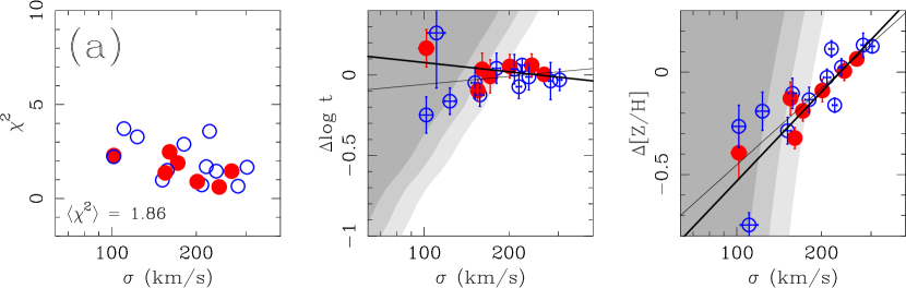
Figure 6.— Stellar population parameters as a function of velocity dispersion for ellipticals (filled red circles) and E/S0 and S0 galaxies (open blue circles) for three different classes of models: (a) where only relative age and metallicity are fit ($\Delta\log t$-$\Delta$[Z/H]); (b) where relative age, metallicity ,and $\alpha$-enhancement are fit ($\Delta\log t$-$\Delta$[Z/H]-$\Delta$[$\alpha$/Fe]); and (c) where relative age, metallicity, $\alpha$-enhancement, and nitrogen-enhancement are fit ($\Delta\log t$-$\Delta$[Z/H]-$\Delta$[$\alpha$/Fe]-$\Delta$[$\alpha$/N]). Only those galaxies with all eight observables are shown. The left-most panels show the reduced $\chi^{2}$ for each galaxy, also plotted against galaxy velocity dispersion. The mean reduced $\chi^{2}$ values are also given in these panels. There are several key features to note: (1) There appears no statistically significant correlation of age with velocity dispersion; (2) there is a clear $\Delta$[Z/H]-$\log\sigma$ correlation; and (3) our correlations of $\Delta$[$\alpha$/Fe] with $\log\sigma$ are marginally significant and they even appear to be anti-correlated when nitrogen is allowed to vary; and (4) The addition of $\Delta$[$\alpha$/N] as a fitted parameter significantly improves the fits to the observed line strengths. The darkest gray region shows the location of the $R=21$ mag selection cut, using the $R$-band Faber-Jackson relation in the cluster. The lighter shades of gray show the +1- and +2-$\sigma$ scatter about the Faber-Jackson relation. In plotting the abundance ratios, we assume the $M/L$ ratios have zero dependency on the specific abundance ratio in order to show the selection. Within these gray regions, the selection effects become important and the sample becomes non-random. As a result, we do not include those galaxies within these biased regions when fitting for population trends with $\sigma$. The thin and thick solid lines show the correlations obtained when fitting using galaxies with velocity dispersions greater than the mean dispersion at $R=21$ mag (134 km/s), and the mean plus one standard deviation (158 km/s), respectively. The abundance trends are insensitive to the selection biases, while apparent correlations of age with velocity dispersion are biased strongly by those galaxies at the limit of the sample. As a result, there is no significant evidence for a correlation of stellar population age with $\sigma$.

4.1. Models with Variable Ages

Here we explore several sets of models in which the relative ages are fit, and in which the parameters controlling the relative abundance ratios are optionally kept frozen. These models will be used to explore to what extent the SSP ages vary among the early-type galaxies in this sample. Figure 6(a) shows results when one fits only for $\Delta\log t$ and $\Delta$[Z/H], and keeps the other four parameters fixed. The filled red circles denote the ellipticals; the open blue circles the E/S0 and S0 galaxies. The morphologies, again, are taken from Fabricant, Franx, & van Dokkum (2000). Because the models have been recalibrated to the data, each index should yield the same ages and abundances. However, the different indices have different sensitivities so data missing for particularly indices can bias the results for those galaxies. Therefore, only those galaxies in the homogeneous sample, with all eight observables, are shown and all discussions of correlations and statistical variations will refer only to these galaxies.

In each of the figures for this section, we plot the best-fit relative stellar population parameters against galaxy velocity dispersion, and also include a panel showing the reduced $\chi^{2}$ of the fit for each galaxy. In the plots of relative age, or metallicity, vs. velocity dispersion, we show the approximate location of magnitude selection cut using three gray tones. The darkest gray region shows the region of velocity dispersions for galaxies below the mean dispersion at $R=21$ mag, using the Faber-Jackson relation of the full sample. The +1- and +2-$\sigma$ scatter of the $R$-velocity dispersion correlation is indicated by the lighter gray strips. In these regions the galaxy selection is no longer random and the sample becomes biased. Therefore, we can not include those galaxies in any calculation of correlations of the parameters with redshift.

In each figure we show the effects of the selection using the thin and thick solid lines, derived by fitting correlations using those galaxies with $\sigma>$ 134, 158 km/s, respectively. These cuts in velocity dispersion represent the mean dispersion, and the mean dispersion plus one standard deviation, at $R=21$ mag. In principle, 50% and 32% of the underlying sample of galaxies at the magnitude limit of $R=21$ mag are lost. Those galaxies at the limit which are over-luminous for their velocity dispersion, either because they are younger or metal poor, can make it into the sample and bias the observed population trends. In fitting for correlations, we opt not to weight using the uncertainties because the measurement errors are significantly correlated with $\sigma$. Uncertainties in the fitted slopes were computed using the “bootstrap” method (with 5000 random samples). We discuss any specific correlations in more detail below.

For the models in which only $\Delta\log t$ and $\Delta$[Z/H] vary, the mean $\chi^{2}$ per degree of freedom for the two-parameter models was $\langle\chi^{2}\rangle=1.86\gg 1$, indicating that such models, in which only these two parameters vary, are not complete descriptors of the stellar populations. However, despite the poor quality of the fitting, the [Z/H]-$\sigma$ relation is apparent. Discussions of the significance of any correlations with $\sigma$ are deferred until below, when fits to the data with lower $\langle\chi^{2}\rangle$ are derived.

In fitting the line strengths we find that the two parameters $\Delta\log t$ and $\Delta\rm[Z/H]$ are insufficient for describing the observations. Therefore, we proceed to add additional parameters, one-by-one. Because of the previously published work incorporating $\alpha$/Fe as a key parameter in the stellar populations of early-type galaxies (e.g., Jørgensen, 1999; Trager et al., 2000b; Proctor et al., 2004a; Thomas et al., 2005), we now allow $\Delta$[$\alpha$/Fe] to vary in the fitting. In Fig. 6(b), these results are shown, again plotted against velocity dispersion. For purposes of illustration, the gray regions of exclusion are plotted assuming that the $M/L$ ratios have zero dependence on the abundance ratios. With $\langle\chi^{2}\rangle=1.92$ it appears that $\alpha$-enhancement, by itself, does not serve to improve the fits to the blue Lick indices. Furthermore, it suggests that $\alpha$/Fe is not an important parameter for defining the sequence of E/S0s in CL1358+62. The ages appear to be uniform and the $\Delta$[Z/H]-$\log\sigma$ correlation is only slightly flatter than in Fig. 6(a). These models indicate that $\alpha$/Fe is a constant in these galaxies, and not a strong function of velocity dispersion.

These models shown in Fig. 6(b) are directly comparable to many previously published studies of early-type galaxies (e.g. Kuntschner, 1998; Trager et al., 2000b; Thomas et al., 2005; Ziegler et al., 2005). A linear least-squares fit to the relative $\alpha$-enhancement as a function of $\log\sigma$ gives a slope of $-0.01\pm 0.18$ dex/dex (the thick line in the figure), compared to the [$\alpha$/Fe] $\propto 0.33\log\sigma$ found by Trager et al. (2000b) or [$\alpha$/Fe] $\propto 0.28\log\sigma$ found by Thomas et al. (2005). While we do not find a statistically significant correlation of $\Delta$[$\alpha$/Fe] in our 3-parameter models, the difference between our result and theirs is discrepant at the 2-$\sigma$ level (even without knowing what the uncertainties in their slope estimates are, and with our comparatively small sample). Further discussion comparing our constraints on [$\alpha$/Fe] with previous results is reserved for §5.1. Nevertheless, adding $\Delta$[$\alpha$/Fe] to the fitting of the blue indices did not reduce $\langle\chi^{2}\rangle$; surely other abundance ratios are more important.

The Thomas, Maraston, & Bender (2003a) models allow three other abundance ratios to be varied. In previously published analyses of line strengths, there has been evidence for variable nitrogen abundance ratios among old stellar populations, and (Burstein et al., 1984; Briley, Cohen, & Stetson, 2002, 2004a) among early-type galaxies specifically (e.g. Carretero et al., 2004). We therefore investigated the impact of the $\Delta$[$\alpha$/N] relative abundance ratios, and the results are shown in Figure 6(c). First, note the significantly lower mean $\chi^{2}$ per degree of freedom, $\langle\chi^{2}\rangle=1.16$, indicating that nitrogen is a key factor in fitting the blue Lick indices (in particular the cyanogen index). Second, there is a strong correlation of the nitrogen abundance ratio with galaxy velocity dispersion. The origins of this correlation will be explored in a later section.

In the models shown in Figure 6, the slope of the correlation of relative age with velocity dispersion is very sensitive to selection biases. Excluding galaxies below $\sigma<158$ km/s, one obtains $\Delta\log t\propto(0.06\pm 0.19)\log\sigma$. If one cuts the sample at the mean dispersion at $R=21$ mag ($\sigma<134$ km/s), one would expect that galaxies which are “young” for their mass/dispersion would make it into the sample, while older galaxies drop out, thus producing a bias of younger ages at lower velocity dispersion. In fact, this bias appears to be present, as one finds a slope of $\Delta\log t\propto(0.38\pm 0.18)\log\sigma$. This bias is not minimized by selecting only those galaxies with velocity dispersions greater than the mean dispersion at the magnitude limit of the sample, but by selecting only those galaxies with dispersions greater than the mean plus at least one standard deviation of the relation that transforms the magnitude limit to a cut along the abscissa. The larger the scatter in the transformation of the magnitude cut to a cut in the dependent variable, the greater the bias in any correlation is.

Because of the above arguments, we conclude there is no significant evidence for a correlation of stellar population age with $\sigma$, down to the limit of our sample. Furthermore, we find no significant difference between the ages of the S0 and elliptical galaxies down to our magnitude limit. Note that this result is consistent with what was found in our analysis of the fundamental plane (Kelson et al., 2000c).

The best fits to the data in which ages are allowed to vary are shown in Fig. 6(c). These data indicate that the stellar populations of the early-type galaxies not only have remarkably uniform ages at fixed velocity dispersion, but that they also follow a tight $\Delta$[Z/H]-$\log\sigma$ correlation. The resulting distributions of $\Delta\log t$, $\Delta$[Z/H], $\Delta$[$\alpha$/Fe], and $\Delta$[$\alpha$/N] with velocity dispersion can be summarized by the following:

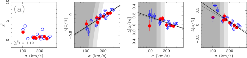
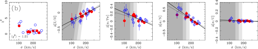
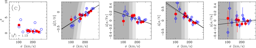
Figure 7.— Same as in Figure 6 but where ages are assumed to be constant. (a) parameters from fitting only for $\Delta$[Z/H], $\Delta$[$\alpha$/Fe], and $\Delta$[$\alpha$/N]; (b) parameters from fitting only for $\Delta$[Z/H], $\Delta$[$\alpha$/Fe], $\Delta$[$\alpha$/N], and $\Delta$[$\alpha$/C]; and (c) parameters from fitting only for $\Delta$[Z/H], $\Delta$[$\alpha$/Fe], $\Delta$[$\alpha$/N], and $\Delta$[$\alpha$/Ca]. No improvements are found by allowing the Ca and C abundance ratios to vary. We find no significant correlation of these abundance ratios with velocity dispersion. The ramifications of the correlations of the nitrogen and carbon abundance ratios with velocity dispersion are discussed in §5.3.

$\bullet$ The scatter in relative ages, above the limit of the sample, is 0.06 dex. The scatter expected from the formal errors is $0.09$ dex, suggesting that the formal errors on the relative ages have been overestimated by a third. The observed scatter is consistent with the low scatter in mass-to-light ratios, at fixed $\sigma$, found in Kelson et al. (2000c). There is no significant correlation of relative age with velocity dispersion, down to the limit of the sample, consistent with the lack of evolution of the fundamental plane slope to this redshift (Kelson et al., 2000c).

$\bullet$ No difference in the relative ages and abundance patterns of Es and S0s is seen in CL1358+62, contrary to what was seen in Fornax by Kuntschner (1998). This is presumably because the Es and S0s in our sample span similar ranges of velocity dispersions, while the S0s in Kuntschner (1998) all have $\sigma<100$ km/s, and, as such, belong to a larger, generally inhomogeneous set of early-type galaxies (e.g. Jørgensen, Franx, & Kjærgaard, 1995; Caldwell & Rose, 1997; Kelson et al., 2000c; Caldwell, Rose, & Concannon, 2003).

$\bullet$ A steep, tight correlation of $\Delta$[Z/H] with velocity dispersion is found, with a slope of $0.86\pm 0.17$ dex/dex. This is about twice as steep as that seen in other samples of early-type galaxies (e.g. Trager et al., 2000b) and we investigate the implications for the color-magnitude relation below. The scatter in $\Delta$[Z/H], at fixed $\sigma$, is $0.06$ dex, where the scatter expected from the formal errors is $0.05$ dex.

$\bullet$ About 30% larger scatter is seen in $\Delta$[$\alpha$/Fe] than the $0.04$ dex expected from the formal errors. There appears to be a mild anti-correlation of $\Delta$[$\alpha$/Fe] with velocity dispersion, with a slope of $-0.44\pm 0.25$ dex/dex. Using those galaxies with $\sigma>134$ km/s, one obtains $-0.28\pm 0.15$ dex/dex, indicating potential sensitivity to the selection. The inclusion of the nitrogen abundance ratio in the fitting does have an impact on the best-fit values for $\Delta$[$\alpha$/Fe], with many of the blue indices providing leverage on [$\alpha$/Fe] (see Table 3 and Thomas, Maraston, & Bender, 2003a; Thomas, Maraston, & Korn, 2004). Without variable nitrogen abundance ratios, one obtains $\Delta$[$\alpha$/Fe] $\propto(-0.01\pm 0.18)\log\sigma$. Such $\alpha$-enhancement patterns differ from previously published correlations of $\Delta$[$\alpha$/Fe] with velocity dispersion (see, e.g. González, 1993; Trager et al., 2000b; Mehlert et al., 2003; Thomas et al., 2005), though earlier work relied on redder Lick indices (e.g. Mg$b$), employed models in which the nitrogen was not free to vary. We discuss the implications of these $\Delta$[$\alpha$/Fe] estimates on the Mg-$\sigma$ relation below.

$\bullet$ A steep anti-correlation of $\Delta$[$\alpha$/N] with velocity dispersion is found, with a slope of $-1.36\pm 0.32$ dex/dex. Using those galaxies with $\sigma>134$ km/s, one obtains $-1.17\pm 0.22$ dex/dex. Given the results for $\alpha$/Fe, we can restate the correlation of nitrogen enhancement with velocity dispersion as $[{\rm N/Fe}]\propto(0.94\pm 0.24)\log\sigma$, or $[{\rm N/H}]\propto(1.78\pm 0.25)\log\sigma$. The implications of the apparent nitrogen-$\sigma$ correlation will be discussed further below, though at a basic level the nitrogen abundance ratio appears to play an important role in dictating the behavior of many blue Lick indices, especially given its impact on the fits for [$\alpha$/Fe]. The scatter in $\Delta$[$\alpha$/N], at fixed $\sigma$, is 0.08 dex where the scatter expected from the errors is 0.06 dex.

4.2. Models with Variable Carbon and Calcium

The results of the fits in the previous section indicate that the ages of the early-types show no statistical variation down to the limit of our selection. Therefore we now fit models in which we forced $\Delta\log t=0$. Fixing the relative ages does not lead to an increase in reduced $\langle\chi^{2}\rangle$, consistent with the scatter in relative ages arising from the formal errors alone. Note that freezing the ages introduces no changes to the correlations of $\Delta$[Z/H], $\Delta$[$\alpha$/Fe], or $\Delta$[$\alpha$/N] with $\log\sigma$ discussed in the previous section. This is shown graphically in Figure 7(a). Note, too, that the mean $\chi^{2}$ per degree of freedom has actually decreased, providing further proof that fitting for the ages does not contribute any statistically significant information about the stellar populations.

Since the relative ages can be constrained without affecting the other parameters, we now explore whether $\Delta$[$\alpha$/C] and $\Delta$[$\alpha$/Ca] have any significant variation among the E/S0s in CL1358+62. Figures 7(b) and (c) show that these additional variables do not improve the quality of the fits to the blue Lick indices, and that the carbon and calcium abundance ratios show no statistically significant variation or correlation with $\log\sigma$. We also verified that the inclusion of these abundance ratios has no effect on the correlations of $\Delta$[Z/H], $\Delta$[$\alpha$/Fe], and $\Delta$[$\alpha$/N] with velocity dispersion shown above.

Given the extreme sensitivity of the C4668 index to both [Z/H] and [$\alpha$/C], we find these results quite remarkable. First, the lack of a correlation of the carbon abundance ratio with velocity dispersion indicates that the broadening corrections were accurate (fitting the uncorrected line strengths leads to an anti-correlation of $\Delta[\alpha/{\rm C}]$ with $\log\sigma$). In the context of the steep correlation of nitrogen abundance with velocity dispersion, constant carbon abundance ratios have important ramifications, to be discussed in the next section. Lastly, though the constraints on the calcium abundances are not strong, we see no evidence for a trend of $\Delta$[$\alpha$/Ca] (or, by extension, $\Delta$[Ca/Fe]) with velocity dispersion, contrary to what has been published by previous authors (Saglia et al., 2002; Cenarro et al., 2003; Falcón-Barroso et al., 2003; Michielsen et al., 2003; Thomas, Maraston, & Bender, 2003b).

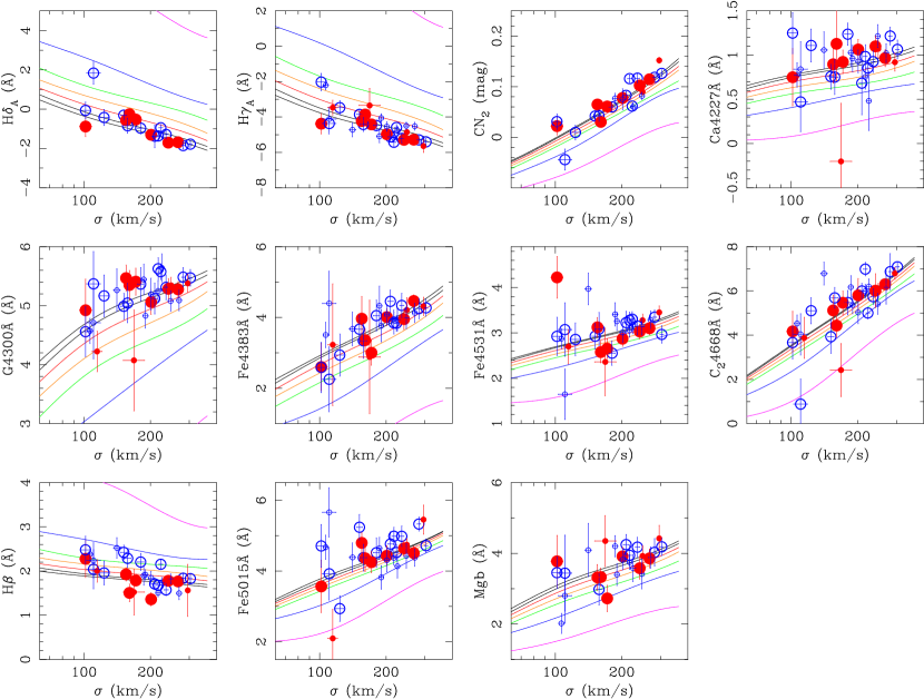
Figure 8.— The line strength-line width relations for E/S0s in CL1358+62. Symbols are as in Figure 5. The solid lines show curves of constant age and constant $\alpha$/Fe, defined by projecting the $\Delta$[Z/H]-, and $\Delta$[$\alpha$/N]-$\sigma$ relations. The ages range from 1 Gyr to 7 Gyr (violet, blue, green, orange, etc.) in increments of 1 Gyr. Several items are worth noting: (1) while H$\beta$, Fe5015, and Mg$b$ were not used in the fitting, the fitted correlations of stellar population parameters with velocity dispersion reproduce the observed H$\beta$-, Fe5015-, and Mg$b$-$\sigma$ relations in CL1358+62 (though Mg$b$ has some residual contamination of telluric absorption); (2) we also show all the E/S0s in the sample, including those galaxies that did not have observations of all of the fitted indices and were not included in the analysis of the homogeneous set of 19 E/S0s discussed in the text; and (3) the slopes of the line strength-line width relations are sensitive to the ages of the galaxies, even when there is no variation of age with velocity dispersion. The Thomas, Maraston, & Bender (2003a) (and Thomas, Maraston, & Korn, 2004) stellar population models do an excellent job of describing the relative properties of the E/S0s in this cluster.

5. Summary of the Model Fitting and Implications

The models explored in this paper indicate: (1) that the ages of the elliptical and lenticular galaxies in CL1358+62 are remarkably homogeneous, consistent with the analysis of the fundamental plane of these galaxies (Kelson et al., 2000c); and (2) the stellar populations in these galaxies obey tight, well-defined [Z/H]-, and [$\alpha$/N]-$\sigma$ relations. Together these trends, when propagated through stellar population models, should reproduce all of the observed early-type galaxy scaling relations in CL1358+62 and to this end we show the observed line strength-line width relations for the sample in Figure 8. Note that the figure also includes those galaxies that did not satisfy our criterion of having measurements for all of the indices fit in the previous discussions, showing a total of 33 E/S0s. This full sample is inhomogeneous in the sense that any galaxy’s stellar population parameters would not necessarily derive from an identical set of indices. Note that along with the eight fitted indices we have also included H$\beta$, Fe5015Å, and Mg$b$ in the figure.

5.1. The Line Strength-Line Width Projections

In the individual line strength-line width diagrams we project the metallicity- and nitrogen-$\sigma$ relations, assuming no correlation of $\alpha$/Fe with velocity dispersion. The lines show loci of constant ages ranging from 1 Gyr to 7 Gyr (the latter essentially the defined age for the reference point used in recalibrating the models to the data; see §3.1). The oldest isochrones clearly reproduce the observed line strength-line width relations well in CL1358+62, and it is worth noting that the slopes of the isochrones are predicted to evolve with age. This “evolution” arises from the nonlinearity of the model grids. The implication is that any observed evolution in the slopes of line strength-line width relations with redshift should not necessarily be taken as proof that stellar population ages vary along the sequence of early-type galaxies.

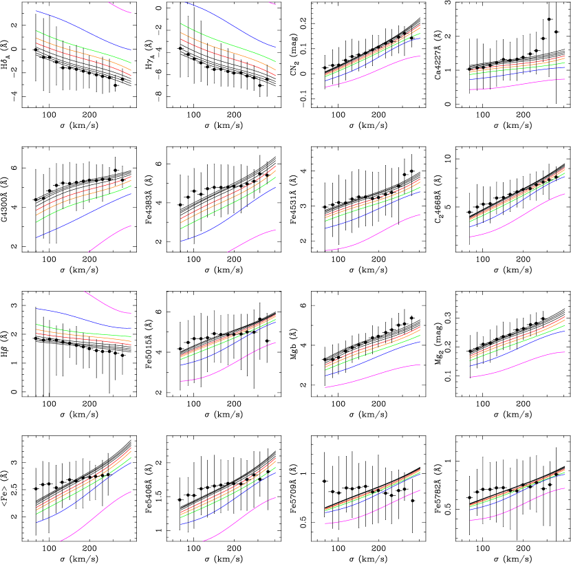
Figure 9.— A comparison of isochrones following the [Z/H]- and [$\alpha$/N]-$\sigma$ relations of the text with selected data from the survey of nearby clusters by Nelan et al. (2005). The points show the median line strengths of those galaxies with OIII equivalent widths less than the median of the sample, binned in velocity dispersion in units of 0.05 dex. The vertical bars show the bounds within which 90% of the sample are distributed. The predicted loci of galaxies agree well with the distribution of galaxies in the nearby clusters for many of the indices. The data of Nelan et al. (2005) show mildly flatter line strength-line width relations for the narrow atomic indices Fe4383, Fe5015, $\langle\rm Fe\rangle$, Fe5406, Fe5709, and Fe5782 in contrast to the excellent match to Fe4383 in Fig. 8. These discrepancies, as well as the divergence of Ca4227 at large dispersion, may be due to differences in the treatment of the broadening corrections as these are the narrowest indices.

Previous analyses of redder Lick indices explicitly relied on Mg line strengths, and strong correlations of [$\alpha$/Fe] with velocity dispersion have been inferred from Mg₂ or Mg$b$ (e.g. Terlevich et al., 1981; González, 1993; Gorgas et al., 1993; Trager et al., 1998; Kuntschner et al., 2001; Sánchez-Blázquez, 2004; Thomas et al., 2005). However, our data simply do not reproduce the long-standing correlation of $\alpha$-enhancement with $\sigma$. The blue line strength-line width relations of the E/S0s in CL13562 are fit well with no correlation, or perhaps even with a mild anti-correlation [$\alpha$/Fe] with $\log\sigma$. Furthermore, we note that despite explicitly excluding H$\beta$, Fe5015, and Mg$b$ from the fitting, their line strength-line width relations are well described by the projections of the abundance-velocity dispersion relations found with the bluer indices (though our Mg$b$ observations have larger scatter due to uncertainties in the corrections for telluric absorption).

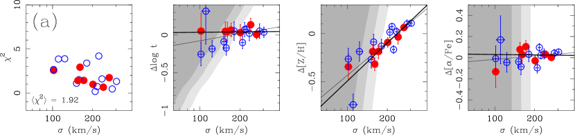
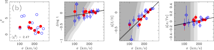
Figure 10.— A comparison of the best-fit parameters $\Delta\log t$, $\Delta$[Z/H], $\Delta$[$\alpha$/Fe] (with no additional nitrogen enhancement) using (a) the line strengths corrected for instrumental and Doppler broadenings using the method in §2.4; (b) the line strengths determined using a traditional approach to correcting the effects of instrumental and Doppler broadenings. Subtle differences in the treatment of the broadening corrections lead to different inferred correlations of $\alpha$-enhancement with velocity dispersion. In (a), the best-fit slope is $[\alpha/{\rm Fe}]\propto(-0.01\pm 0.18)\log\sigma$, while in (b), the best-fit slope is $[\alpha/{\rm Fe}]\propto(+0.27\pm 0.13)\log\sigma$, more consistent with previously published results.

Our estimates of $\alpha$/Fe have implications for the origin of the Mg₂-, Mg$b$-, and $\langle\rm Fe\rangle$-$\sigma$ relations (Thomas et al., 2005, e.g.). Using the models we can recast the metallicity- and nitrogen-$\sigma$ correlations as Mg-$\sigma$ relations and test whether our results are consistent with previous measurements of its slope (though the nitrogen has no impact on the Mg indices in the current incarnations of the models). After passively evolving these relations to the present epoch, we find Mg${}_{2}\propto(0.23\pm 0.05)\log\sigma$, in excellent agreement with that found nearby (typical slopes nearby range from 0.17 to 0.23 mag/dex; Worthey & Collobert, 2003). For Mg$b$, the Thomas, Maraston, & Bender (2003a) and Thomas, Maraston, & Korn (2004) models predict that Mg$b$ is about twice as sensitive to changes in $\alpha$/Fe, so a comparison to Mg$b$ should provide a stronger test of the consistency of our results with previously published data. We infer Mg$b\propto(2.8\pm 0.7)\log\sigma$, consistent with the Mg$b\propto 2.8\log\sigma$ typically seen (see Worthey & Collobert, 2003). Fitting the Mg$b$ data of the full inhomogeneous sample directly, we obtain Mg$b\propto(2.1\pm 0.8)\log\sigma$ (see Fig. 8).

Because our results are consistent with the Mg$b$-$\sigma$ (and Mg₂-$\sigma$) relation, we now explore potential sources of the discrepancy over $\alpha$/Fe. In Figure 9 our [Z/H]- and [$\alpha$/N]-$\sigma$ correlations have been propagated through the models and plotted over data taken in a survey of nearby clusters from Nelan et al. (2005). Those authors observed more than 4000 red-sequence galaxies in 93 low-redshift clusters. Because of the large number of galaxies in their survey, and the low typical signal-to-noise ratio of their spectra, we bin their data in intervals of 0.05 dex, and use only those galaxies with minimal detected OIII emission. The vertical bars mark the bounds within which 90% of the galaxies fall. The points show the median line strength within each bin.

Overall the comparison between the Nelan et al. (2005) data and the predicted line strength-line width relations is quite good. However there are particularly interesting discrepancies: the relations for Fe4383, Fe5015, and $\langle\rm Fe\rangle$, Fe5406, Fe5709, Fe5782. For these indices, our best-fit stellar population trends produce steeper slopes than observed in the Nelan et al. (2005) data. Because $\langle\rm Fe\rangle$ has historically been one of the primary constraints on metallicity, we conclude that the shallow slope of the $\langle\rm Fe\rangle$-$\sigma$ relation of Nelan et al. (2005) is characteristic of the kinds of relations that have led to flatter [Fe/H]-$\sigma$ relations than indicated by our data. Such a flat [Fe/H]-$\sigma$ relation invariably necessitates a positive correlation of [$\alpha$/Fe] with velocity dispersion in order to match the slope of the Mg$b$-$\sigma$ relation. As can be seen in Fig. 8, our Fe4383-$\sigma$ relation (and Fe5015-$\sigma$, though with larger scatter) has a slope that agrees with the projection of the models, thus, in tandem with the other indices, negating the need for a significant correlation of $\alpha$/Fe with velocity dispersion. Clearly the primary source of the discrepancy in $\alpha$/Fe comes from the narrow Fe indices. Note, too, the divergence of Ca4227 at large values of $\sigma$.

These discrepant indices are some of the narrowest in the Lick system, and because the remaining indices (those that require very small corrections) are matched very well by our abundance patterns, one must suspect that the discrepancy in $\alpha$/Fe-$\sigma$ arises from differences in the treatment of the corrections for instrumental and Doppler broadening. These narrow indices have had large, systematic corrections for Doppler broadening applied to them by Nelan et al. (2005) (see, e.g., Poggianti et al., 2001, for plots of such corrections as functions of velocity dispersion). Systematic errors in such corrections can modify the inferred slopes of line strength-line width relations.

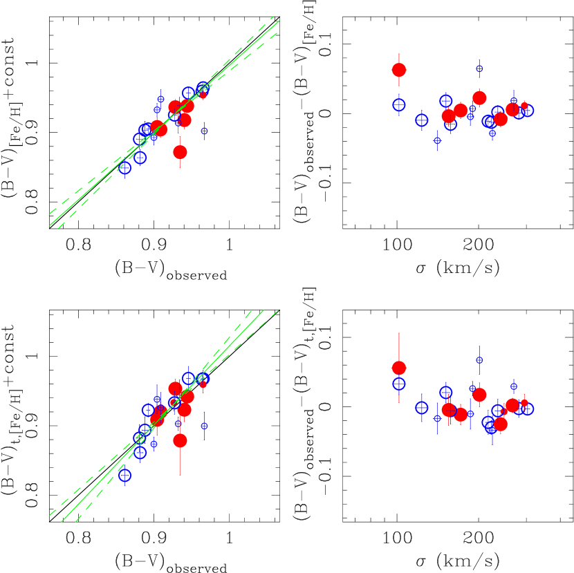
Figure 11.— A comparison of observed restframe $(B-V)_{\rm observed}$ colors (Kelson et al., 2000a, c) with those predicted using the best-fit stellar population parameters (Bruzual & Charlot, 2003). The top panels show predicted colors derived when age was kept constant. The bottom panels show the predicted colors when age was allowed to vary. In the left-hand panels the black solid line indicates a slope of unity. When only the abundances were allowed to vary, the best-fit slope is $(B-V)_{\hbox{\small[Z/H]}}\propto(0.97\pm 0.11)(B-V)_{\rm observed}$, shown by the green solid line (where the 1-$\sigma$ uncertainties are shown using the green dashed lines). When age is allowed to vary one obtains $(B-V)_{\hbox{\small t,[Z/H]}}\propto(1.14\pm 0.16)(B-V)_{\rm observed}$, also shown in green. The effects of including age are small because of (1) the statistically insignificant variations in age in the sample, and (2) the large covariances between [Z/H] and $\log t$ and the age-metallicity degeneracy in $(B-V)$ colors. The differences between the observed and predicted colors are shown plotted against velocity dispersion in the right-hand panels. The residuals in the colors are remarkably small, consistent with the formal uncertainties.

We tested whether the different $\alpha$/Fe-$\sigma$ correlation was an inherent property of the sample or whether the treatment of the corrections played a role. For the first test we derived line strengths using the traditional method, i.e. first smoothing the spectra to the resolution of the IDS, then measuring the indices, and finally applying multiplicative corrections to these measurements. These velocity dispersion corrections were constructed using an old, metal-rich Bruzual & Charlot (2003) model SED. These line strengths were propagated through the machinery to derive new stellar population parameters and the results are compared in Figure 10 to the parameters found earlier. As can be seen in Fig. 10(b), we recovered $\Delta$[$\alpha$/Fe] $\propto(+0.27\pm 0.13)\log\sigma$, in much better agreement with previously published correlations. In this test, the corrections were computed using a single template. Using the best-fit Bruzual & Charlot (2003) SED for each galaxy instead of a single template, we find no significant change in the slope of the inferred correlation (though the scatter is larger).

Given this discrepancy, we performed a second test of our broadening corrections by smoothing the galaxy spectra to have intrinsic broadenings equivalent to the Lick/IDS resolution with zero velocity dispersion, i.e. by subtracting, in quadrature, the velocity dispersion from the IDS resolution. We remeasured the indices in these spectra and compared them to our broadening-corrected indices derived earlier. We found no statistically significant systematic differences between these measurements and the measurements corrected in §2.4, for the line strengths of those galaxies with velocity dispersions less than the IDS resolution at the wavelength of a given central passband. Therefore we conclude that our treatment of the broadening corrections has not introduced any gross systematic errors as a function of velocity dispersion.

Lastly, it is worth re-emphasizing that our diagnostics of $\alpha$-enhancements differ from those traditionally used. For example, our spectral coverage does not provide direct constraints on magnesium abundances. The blue indices should have stronger (though indirect) sensitivities to oxygen abundances, primarily through the CNO equilibrium in the atmospheres of cool giants. Because oxygen is the dominant $\alpha$ element, our absence of a correlation of $\alpha$/Fe with velocity dispersion may be a more accurate descriptor of the behavior of $\alpha$ elements than indicated by Mg alone (though we note the excellent match to the slopes of published Mg-$\sigma$ relations). In other words, our $\alpha$/Fe results may simply reflect more on a uniformity in O/Fe than in Mg/Fe, not to mention our empirically constrained uniformity in the carbon and calcium abundance ratios.

While the broadening corrections appear to play an important role in the determinations of $\alpha$/Fe in the 3-parameter fitting, these corrections become less important when including the nitrogen enhancement. When using the line strengths corrected for broadening via the traditional method, we obtain similar results to those shown in Figure 6(c) for the 4-parameter fitting of age, metallicity, $\alpha$/Fe, and N/$\alpha$. In §5.3 the inferred nitrogen-$\sigma$ correlation will be discussed in more detail, coming to the conclusion that it has a natural origin.

In the next section we show that the observed colors of the galaxies match those predicted by the stellar population parameters that we have derived.

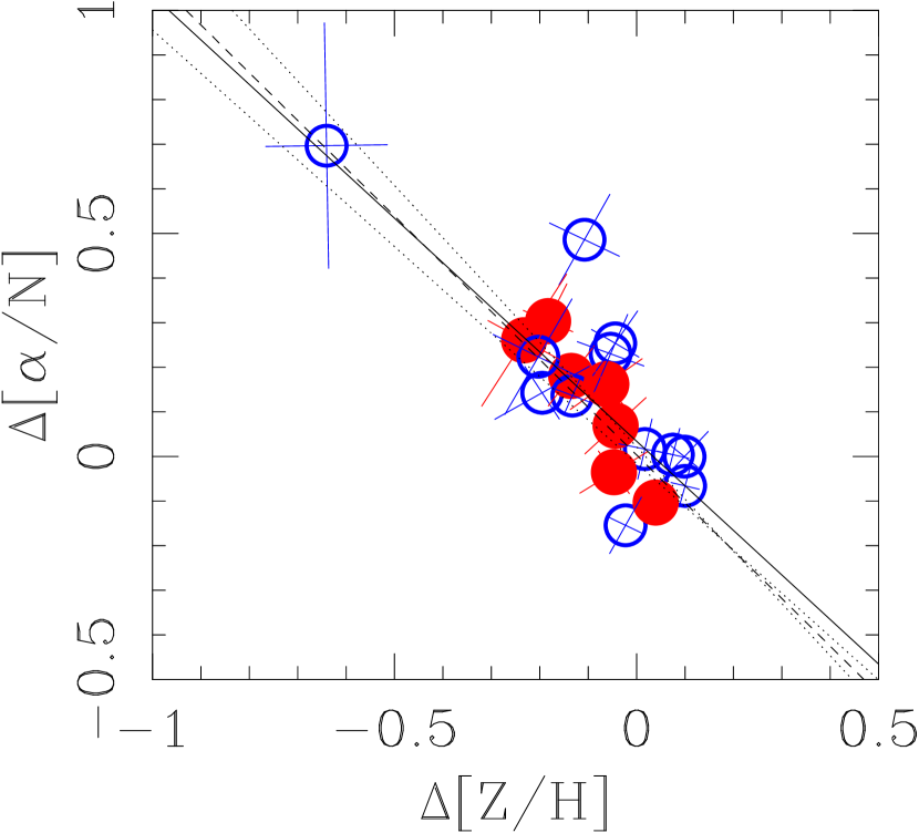
Figure 12.— The correlation of $\Delta[\alpha/{\rm N}]$ and $\Delta[{\rm Z/H}]$. For simple models of chemical enrichment (Köppen & Edmunds, 1999; Henry, Edmunds, & Köppen, 2000; Köppen & Hensler, 2005) in which abundances are dominated by secondary nitrogen, one expects the relation to follow $\Delta[\alpha/{\rm N}]=-\Delta[{\rm Z/H}]$, shown by the solid line. We fit for the best-fit linear relation, using those galaxies with $\sigma>134$ km/s, by minimizing the squares of the residuals parallel to both axes of the error ellipses simultaneously. The resulting best-fit slope is $(-1.07\pm 0.10)$ dex/dex, shown by the dashed and dotted lines. The agreement between the stellar population parameters and the prediction of simple chemical evolutionary models is striking. Note that this slope was derived using galaxies above the limit of the selection, and thus excluded, for example, galaxy 493 with the lowest metallicity and highest nitrogen abundance.

5.2. The Color-Magnitude Relation

The [Z/H]-$\sigma$ correlation has strong implications for the color-magnitude relation. We explore these using the WFPC2 data published by van Dokkum et al. (1998a) and Kelson et al. (2000a). These images were convolved with Gaussians to mimic the seeing in our spectroscopy. Then $\rm(F606W-F814W)$ colors were measured within circular apertures similar to the apertures used for the spectral extractions. The colors were transformed to restframe Johnson colors, $(B-V)_{\rm observed}$. In this section we compare these observed colors to those predicted by the Bruzual & Charlot (2003) stellar population models using ages and metallicities from our analysis. In order to eliminate any systematic errors in the photometric transformation, in the calibration, or in the uncertainties in the absolute ages and metallicities, we applied an offset to the colors computed using the biweight estimator of Beers, Flynn, & Gebhardt (1990), much like what was done earlier for the line strength fitting.

Figure 11 shows a comparison of these predicted colors with the observed $(B-V)_{\rm observed}$ colors. When the ages were kept constant, we refer to the predicted colors as $(B-V)_{\hbox{\small[Z/H]}}$. When the ages were allowed to vary in the fit, the predicted colors are referred to as $(B-V)_{\hbox{\small t,[Z/H]}}$.

In the left-hand panels one finds that both sets of predicted colors match the observed colors well. Simple fits to the comparisons yield $(B-V)_{\hbox{\small[Z/H]}}\propto(0.97\pm 0.11)(B-V)_{\rm observed}$, and $(B-V)_{\hbox{\small t,[Z/H]}}\propto(1.14\pm 0.16)(B-V)_{\rm observed}$, and these are shown using the green lines. The solid black line indicates a slope of unity. Because colors suffer from an age-metallicity degeneracy similar to that which plagues the absorption line strengths, the comparison of the colors only serves as a sanity check — stellar populations are indeed redder as they become older or more metal-rich, and in the correct proportion to the changes in spectroscopic ages or metallicities. In other words, one gains no additional leverage on the stellar population parameters by fitting $(B-V)$ colors with the absorption line strengths.

Simply put, the fitted ages and metallicities reproduce the color-velocity dispersion relations remarkably well. In the right-hand panels we plot the color residuals against $\sigma$, and the very low scatter, $\pm 0.02$ mag, is consistent with the formal uncertainties.

Had the ages and metallicities from Figure 10(b) been used, the slopes of the correlations between the predicted and observed colors would have resulted in slopes of $(B-V)_{\hbox{\small[Z/H]}}\propto(1.25\pm 0.10)(B-V)_{\rm observed}$, and $(B-V)_{\hbox{\small t,[Z/H]}}\propto(1.50\pm 0.17)(B-V)_{\rm observed}$, with significantly larger scatter. This is because a significant, positive correlation of $\alpha$-enhancement with velocity dispersion decreases the slope of the [Z/H]-$\sigma$ correlation to the point that the color-velocity dispersion relation can no longer be matched.

In summary, the colors predicted by our population parameters are in excellent agreement with the observed colors, when measured in the appropriate aperture. This remarkable consistency between the colors and the spectroscopic properties of these galaxies also implies that dust is not an important contributor to the colors of early-type galaxies.

5.3. The Nitrogen Relation

In fitting the Thomas, Maraston, & Bender (2003a) models to the blue line strengths, we found a strong apparent correlation of nitrogen enhancement with velocity dispersion. However, there appears to be no associated correlation (or anti-correlation) with the carbon abundance ratio. The lack of concordance between the nitrogen and carbon enhancements was not expected. Taken together with our inability to reproduce the previously published correlation between [$\alpha$/Fe] and $\log\sigma$, our results would seem to indicate either fundamental problems with the stellar population models, or something truly fundamental about the formation and enrichment histories of galaxies.

Certainly, uncertainties in the models are important (see e.g. Gratton, Sneden, & Caretta, 2004, for a review of unexplained C and N variations among globular clusters). The nitrogen- and carbon-sensitive indices, are affected by mixing from first dredge-up, by other mixing processes as well (again, see Gratton, Sneden, & Caretta, 2004, for a thorough summary and detailed references), and by the unknown abundances of oxygen, which are a wholly separate canard on their own (Bensby, Feltzing, & Lundström, 2004; Proctor et al., 2004; Thomas et al., 2005). Recent work on understanding the carbon and nitrogen abundances in Galactic and globular clusters continue to confound (e.g. Aoki & Tsuji, 1997; Bellman et al., 2001; Briley, Cohen, & Stetson, 2002, 2004a), though it appears likely that both pollution by early generations of intermediate-mass asymptotic giant branch (AGB) stars (Briley et al., 2004b, e.g.) and additional mixing processes (e.g. Boothroyd & Sackmann, 1999) occur. Taken all together, one cannot rule out if the deduced N/C correlation with velocity dispersion is an artifact arising from an absence of processes that modify the atmospheric abundance ratios in the models, processes that are themselves sensitive to metallicity (e.g. Charbonnel, 1994; Bensby, Feltzing, & Lundström, 2004).

Recalibration of the models to the data eliminated several systematic errors, as illustrated in Appendix A, and as a result, the relative measures of age and abundance are probably quite reasonable. However, the N/C ratios may yet be reflecting limitations in the stellar libraries and fitting functions (Worthey, 1994; Thomas, Maraston, & Bender, 2003a; Thomas, Maraston, & Korn, 2004), in that the parameter space of second derivatives of the indices has not yet been fully explored and modeled (Tripicco & Bell, 1995; Korn, Maraston, & Thomas, 2005). Sufficiently large, but unmodeled, non-linearities in the underlying sensitivities of the indices could be invoked to eliminate the nitrogen abundance trends but the efforts to calibrate the models using the integrated light of globular clusters (e.g. Schiavon et al., 2002; Thomas, Maraston, & Bender, 2003a; Proctor et al., 2004) provide some confidence in our results.

It is worth noting that the more common line strength-line width relations, such as Mg-$\sigma$, appear to be well-described without any need for a correlation of $\alpha$-enhancement with velocity dispersion, all while the blue Lick indices are fit quite well. This self-consistency did, however, come at a cost: that of throwing away the zero-points of the models and the absolute measures of abundance and age. Had we not done so, the reduced $\chi^{2}$ on individual galaxies increase by factors of 2–7! Taken together with the large systematic uncertainties shown in the appendix, we have much greater confidence in the relative measures of abundance derived above than in estimates of absolute abundances.

The steep correlation of the nitrogen abundance ratio with velocity dispersion has interesting implications, but perhaps not for the most obvious reason. Naively one might invoke a physical correlation between gravitational potential and the timescales and/or efficiency of star-formation (e.g. Henry & Worthey, 1999; Worthey, 1998; Henry, Edmunds, & Köppen, 2000) given the sensitivities of nitrogen abundances to these parameters for closed-box models. However, the underlying correlation for nitrogen is probably not with velocity dispersion per se but with mean metallicity: secondary nitrogen is produced in intermediate-mass AGB stars (e.g. Henry, Edmunds, & Köppen, 2000) and the yields are metallicity-dependent (Marigo et al., 1998). Closed-box (and partially closed-box) models of chemical enrichment with modest or high metallicities have N/O ratios dominated by secondary nitrogen such that $\Delta{\rm[N/O]}\propto\Delta{\rm[O/H]}$ (e.g. Köppen & Edmunds, 1999; Henry, Edmunds, & Köppen, 2000; Köppen & Hensler, 2005). The dependency of the yields on metallicity sets the absolute zero-point of the logarithmic relation, but one expects the relation between relative nitrogen abundance ratios and mean metallicities to have unity slope. From the tables in Henry, Edmunds, & Köppen (2000), the carbon yields of AGB stars do not appear to be particularly sensitive to metallicity; presumably this is why our carbon abundance ratios do not correlate with velocity dispersion (or metallicity) in the same way that nitrogen does.

The hypothesis that the $\alpha$/N-$\sigma$ relation is due to secondary nitrogen can be tested because [N/O] is predicted to correlate with [O/H]. Within the context of our data, [$\alpha$/N] is simply a surrogate for [O/N]. Furthermore, even though oxygen abundances cannot be directly measured, our findings of $\Delta[\alpha/{\rm Fe}]\sim 0$ (or $\Delta[{\rm O/Fe}]\sim 0$) imply that we can approximate $\Delta{\rm[Z/H]}\sim\Delta{\rm[O/H]}$. In Figure 12, the relative nitrogen abundance ratios $\Delta[\alpha/{\rm N}]$ against $\Delta[{\rm Z/H}]$. Finding the best-fit relation between $\Delta[\alpha/{\rm N}]$ and $\Delta[{\rm Z/H}]$ is complicated by the correlated errors in the derived abundances so we chose to minimize the squares of the residuals parallel to both axes of the error ellipses simultaneously. We find that the slope of the correlation is $(-1.07\pm 0.10)$ dex/dex, shown by the dashed and dotted lines in the figure. Using other approaches to fit the correlation led to similar results. We therefore conclude that our data are consistent with the hypothesis that the [$\alpha$/N]-$\sigma$ correlation arises from the dependence of yields of secondary nitrogen on metallicity.

The stellar populations of the E/S0 galaxies in CL1358+62 have essentially been reduced to a one-parameter family, obeying a $[{\rm Z/H}]$-$\sigma$ relation. While the presence of (secondary) nitrogen in proportion to the metallicity indicates that the galaxies experienced star-formation over an extended period of time, absolute calibration of the abundances are required in order to derive constraints on the timescales of astration. Even without absolute calibrations, it bears repeating: the populations of both lenticulars and ellipticals have statistically identical relative ages, span similar ranges of metallicity, obey identical [Z/H]-$\sigma$ relations, and show strong evidence for the presence of secondary nitrogen.

Our results conclusively show that cluster S0s did not form their stars at significantly later epochs than cluster ellipticals of the same mass, and the presence of secondary nitrogen indicates that both Es and S0s formed from ancestors with extended star-formation histories. If our $\alpha$/Fe results are correct, then this star-formation must have been sufficiently extended, within a given galaxy, such that the relative proportions of by-products of Type Ia to Type II supernovae are effectively constant, and not strongly dependent on galaxy mass. Furthermore, if the gravitational potential is an important factor in the retention or ejection of enriched materials (e.g. Burke, 1968, and much subsequent work), then material from all energetic sources of enrichment have roughly comparable efficiencies of ejection from the host galaxies, either because of generally low probabilities of ejection, or because the enriched interstellar gas is well-mixed before it either forms the next generations of stars or escapes from its host.

This produces an apparent contradiction with the observed evolution in the morphology-density relation (Dressler et al., 1997; Postman et al., 2005), in which fewer S0s exist at higher redshift (though see Holden et al., 2006), even though the timescales and mechanisms with which S0s form must be very similar to the timescales mechanisms for the formation of ellipticals of the same mass.

Ultimately, the chemical signatures, and any evolution thereof, must be placed in the context of cosmological models. In $\Lambda$CDM, galaxies form hierarchically, through multiple generations of mergers (Kauffmann et al., 1993, 1999; Romeo et al., 2005; Lanzoni et al., 2005; Tran et al., 2005). Unfortunately, multiple major merger events can have a large impact on the observed scaling relations (e.g. Kaviraj et al., 2005), such as the line strength-line width relations analyzed here. Furthermore, (e.g. Juneau et al., 2005) directly measured the star-formation rates of galaxies with these masses over redshifts of $0.8<z<2$ and found that their star-formation has essentially ceased by $z\lower 1.29167pt\hbox{$\scriptscriptstyle\;\buildrel>\over{\sim}\;$}1.5$. In a subsequent paper we will try to address these issues by analyzing the stellar populations of both early- and late-type galaxies in a sequence of five clusters from $z=0$ to $z=0.83$, referencing them to the galaxies presented in this paper. Together it is hoped that these five clusters can provide a more detailed picture of the formation histories of cluster galaxies than can be derived from a snapshot at a single epoch.

6. Conclusions

We have measured absorption line strengths for galaxies in the cluster CL1358+62 using the spectra published in Kelson et al. (2000b). A homogeneous population of early-type galaxies has been analyzed, with the full selection of galaxies in Kelson et al. (2000b) to be discussed in a subsequent paper. The largest source of systematic errors that plague the analysis of absorption lines has been eliminated by matching the stellar populations models (Thomas, Maraston, & Bender, 2003a; Thomas, Maraston, & Korn, 2004) to the mean observed line strengths of the most massive early-type galaxies in CL1358+62. Furthermore, not only does a recalibration of the models allow for accurate differential measurements of the stellar population parameters, but the topology of the $\chi^{2}$ minimum can be used to accurately estimate formal errors.

Using only those E/S0 galaxies which have accurate measurements of eight blue Lick/IDS indices (H$\delta_{A}$, H$\gamma_{A}$, CN₂, Ca4227, G4300, Fe4383, Fe4531, and C4668), we fit for the relative measures of age and chemical abundances. The fitting has resulted in homogeneous sets of stellar population parameters relative to the reference point used in resetting the model zero-point.

The key results can be summarized as follows:

(1) The populations of the E and S0 galaxies are statistically identical in their age and abundance patterns, down to the magnitude limit of $R=21$ mag, consistent with what was found using the fundamental plane (Kelson et al., 2000c). Beyond the magnitude limit, selection biases become important.

(2) The observed scatter in relative ages is 0.06 dex, where the scatter expected from measurement errors is 0.09 dex. The scatter in ages is consistent with that inferred from the color-magnitude relation (van Dokkum et al., 1998a), and from the fundamental plane (Kelson et al., 2000c).

(3) We find a tight correlation between relative metallicity and velocity dispersion, with a slope of $0.86\pm 0.17$ dex/dex. The scatter about this relation is 0.06 dex, where the scatter expected from the formal errors is 0.05 dex. The observed $B-V$ colors are also consistent with the inferred ages and metallicities.

(4) The scatter in relative $\alpha$-enhancement is only 30% larger than expected from the formal errors alone. When the nitrogen abundance ratio is allowed to vary, we find a mild anti-correlation of $\Delta$[$\alpha$/Fe] with $\log\sigma$, but with a significance less than $<2\sigma$. While we find little evidence for a significant correlation (or variation) of [$\alpha$/Fe] with velocity dispersion, the slope of the local Mg-$\sigma$ relation can be reproduced by our $\Delta$[Z/H]-$\sigma$ correlation. Thomas et al. (2005) argued that Mg$b$-$\sigma$ arises mostly from the correlation of metallicity with velocity dispersion. Our results go beyond that and suggest that no variation of $\alpha$/Fe is required. The discrepancy between our conclusions and previously published work on this topic arises from our steeper [Z/H]-$\sigma$ relation. This discrepancy may be due to the treatment of the broadening corrections, in particular for the narrow Lick iron indices, though more detailed analysis is required to verify this hypothesis. Previous work (e.g. Trager et al., 2000b) indicated that cluster E/S0s form a three-parameter family of objects, with [Z/H] and $\alpha$/Fe correlated with velocity dispersion. Historically, models with variable ratios of Type I and Type II supernovae and subsequent galactic winds have been invoked to explain such a complex family of objects. Elimination of the correlation of $\alpha$-enhancement with velocity dispersion would greatly simplify models of E/S0 formation.

(5) We find that the enhancement of nitrogen is strongly correlated with velocity dispersion, while carbon abundance appears to show no variation. This N-$\sigma$ correlation has not been observed before. This new correlation originates either in deficiencies in the stellar population models, or implies new physics to be incorporated into our understanding of E/S0 formation and evolution. The most likely explanation is one in which the nitrogen abundance ratios do not arise from mechanisms specifically tied to $\sigma$, but that the nitrogen-enhancement is correlated with metallicity. In other words, the nitrogen is secondary in origin, and the progenitors of E/S0 galaxies experienced significantly extended star-formation.

These data form the only sample of early-type galaxies in which these particular abundance patterns have been found, so far. In all other respects the sample shows the uniform age distribution and a steep correlation of mean metallicity with velocity dispersion inferred from other diagnostics.

While models which include variable abundance ratios (e.g. Trager et al., 2000b; Thomas, Maraston, & Bender, 2003a; Thomas, Maraston, & Korn, 2004) are relatively immature, their development has been encouraging, and the data are already well-fit by such models. The blue Lick indices appear to be powerful diagnostics of stellar population ages and provide excellent, self-consistent fits to the metal lines, even if the resulting abundance ratios run counter to much of the previous literature. Despite these discrepancies, the observed line strength-line width relations of nearby galaxies, published by Nelan et al. (2005), are recovered, with some notable exceptions. Those relations that match well do bolster our faith in these findings. However, nearly all of the iron line strength-line width relations are not matched well, and the published data on nearby galaxies have had large multiplicative Doppler corrections applied. We suggest that perhaps past treatment of these corrections may be in error. That the $(B-V)$ colors are consistent with our stellar population parameters not only reinforces our conclusions, but also indicates that dust is not an important component in the optical SEDs of early-type galaxies.

The results on enhancements (over Fe) of $\alpha$, nitrogen, and carbon have important implications. While it remains to be seen whether the carbon- and nitrogen-sensitive indices are being modeled correctly, the nitrogen enhancement-velocity dispersion correlation agrees very well with the correlation of [N/Z] with [Z/H] expected to arise from secondary production of nitrogen by AGB stars. Taken together, our differential stellar population parameters suggest that these massive early-type galaxies form a family with only a single parameter: galaxy velocity dispersion (or possible mass).

The uniform ages and simple trends of metallicity with velocity dispersion appear to contradict the observation that fewer S0s exist at higher redshift (Dressler et al., 1997; Postman et al., 2005). We conclude that the timescales and mechanisms with which the populations in S0s form are statistically identical to that of ellipticals of the same mass. Early-type galaxies, now shown to have significant self-enrichment and extended star-formation histories, must be reconciled with hierarchical formation (e.g. Kauffmann et al., 1993) in a $\Lambda$CDM universe. The uniform ages and tight mass-metallicity relation may not be compatible with significant merging and histories of extended star-formation.

In a subsequent paper, we will employ our machinery for measuring these age and abundance patterns in a range of clusters from $z=0$ to $z=0.83$. With comparisons of the properties of cluster galaxies over a range of redshifts, we will test the universality of some of the conclusions presented here, quantify changes in the stellar population parameters with cluster redshift (see, e.g., Kelson et al., 2001; Jørgensen et al., 2005; Barr et al., 2005), and attempt to reconcile the above results with a coherent picture of the formation and evolution of galaxies in rich clusters.

Appendix A The Effects of the Systematic Recalibration

A.1. Differential versus Absolute Population Parameters

In this section we show several figures to illustrate the effects of recalibrating the models to our data. In particular we compare figures shown earlier to variants in which this step is ignored.

Figure 13 shows the parameters of the best-fit models, in which age, metallicity, $\alpha$-enhancement, and nitrogen enhancement are allowed to vary. Figure 13(a) is identical to Fig. 6(c). In Figure 13(b) we show the parameters derived when the zero-point uncertainties are ignored and the models and data are assumed to be on the same system. Similar trends are seen in both the differential and absolute parameters. However the absolute parameters, derived when the recalibration is skipped, have 30–40% larger scatter. These systematic uncertainties appear not to destroy the general trends of the SSP parameters with velocity dispersion but artificially inflate the inhomogeneities in the inferred properties of the stellar populations.

In Figure 14 we show another comparison of the differential and absolute analyses, in particular investigating the effects on parameter-parameter correlations. For this discussion we exclude those galaxies below $\sigma=134$ km/s to reduce the impact of the luminosity-selection bias. In the left-hand panels we show the relative ages and nitrogen enhancements plotted against relative metallicity. No significant correlation exists between the relative ages and relative metallicity. The significant correlation between relative nitrogen enhancements and metallicity was discussed earlier. If one ignores the recalibration of the models to our data, one obtains an anti-correlation between age and metallicity with a slope of $-0.76\pm 0.10$ dex/dex (shown by the dashed and dotted lines). Note that this artificially induced slope obeys the famed “3/4” rule of Worthey (1994) because the systematic errors in our line strengths couple with the average age-metallicity degeneracy of the indices.

Furthermore, in the absolute analysis the correlation between nitrogen enhancement and metallicity effectively disappears. Because Fig. 13(b) shows the strong [Z/H]-$\sigma$ and [N/$\alpha$]-$\sigma$ correlations, a lack of an observed correlation between [Z/H] and [N/$\alpha$] would therefore have masked the true nature of the [N/$\alpha$]-$\sigma$ correlation. Note that while the general trends of the SSP parameters with velocity dispersion were preserved when the recalibration was ignored, the systematic errors in the calibration had resulted in larger errors in the SSP parameters. These errors appeared in Figure 13(b) as larger scatter and increased inhomogeneity. However, these added errors can be both correlated and uncorrelated, possibly imposing apparent (anti)correlations between age and metallicity, or erasing underlying correlations between metallicity and abundance ratios.

For samples of galaxies at high redshift, it remains technical challenge to ensure that absorption line strengths from the models and data have no systematic offsets. Extreme care must be taken to eliminate all sources of systematic error in order to utilize the models’ absolute scales of age and abundance. Fortunately, these large systematic sources of error can be eliminated if one is only interested in the relative properties of galaxies within an homogeneous sample.

A.2. Uncertainties in the Adopted Model Zero-point

In §3.1 we adopted a set of parameters describing the mean stellar population of the most massive E/S0 galaxies in CL1358+62. These parameters are reprinted as Model 0 in Table 5. Here we investigate some of the effects one obtains by varying the parameters of this reference point. Table 5 lists the standard parameters and the three additional variations, Models A, B, and C. These variations are not meant as formal uncertainties in age, [Z/H], or $\alpha$-enhancement, but were specifically chosen to be significantly larger than the uncertainties in those parameters. As a result, the general effects on our results may be considered very conservative systematic uncertainties in our conclusions. Also note that models in which the reference point has solar metallicity and solar $\alpha$/Fe have been ruled out by many authors.

Figure 15 shows the best-fit relative stellar population parameters plotted against velocity dispersion, just as in Figure 6(c). No change in slope in any of the correlations of SSP parameters with velocity dispersion is statistically significant. Because the true uncertainties in the zero-point are likely to be much smaller than the range probed by our variations in age, metallicity, and $\alpha$-enhancement, we conclude that our results are not sensitive to systematic uncertainties in the recalibration.

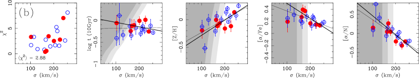
Figure 13.— The effects of ignoring the model recalibration on the stellar population parameters as functions of velocity dispersion for ellipticals (filled red circles) and E/S0 and S0 galaxies (open blue circles). Only those galaxies with all eight observables are shown. (a) $\Delta\log t$-$\Delta$[Z/H]-$\Delta$[$\alpha$/Fe]-$\Delta$[$\alpha$/N] models. (b) $\log t$-[Z/H]-[$\alpha$/Fe]-[$\alpha$/N] models. The left-most panels show the reduced $\chi^{2}$ for each galaxy, also plotted against galaxy velocity dispersion. The mean reduced $\chi^{2}$ values are also given in these panels. While the general trends shown in Figure 6 are clearly visible, the scatter about the correlations is 30–40% larger when the models are not recalibrated to the data.

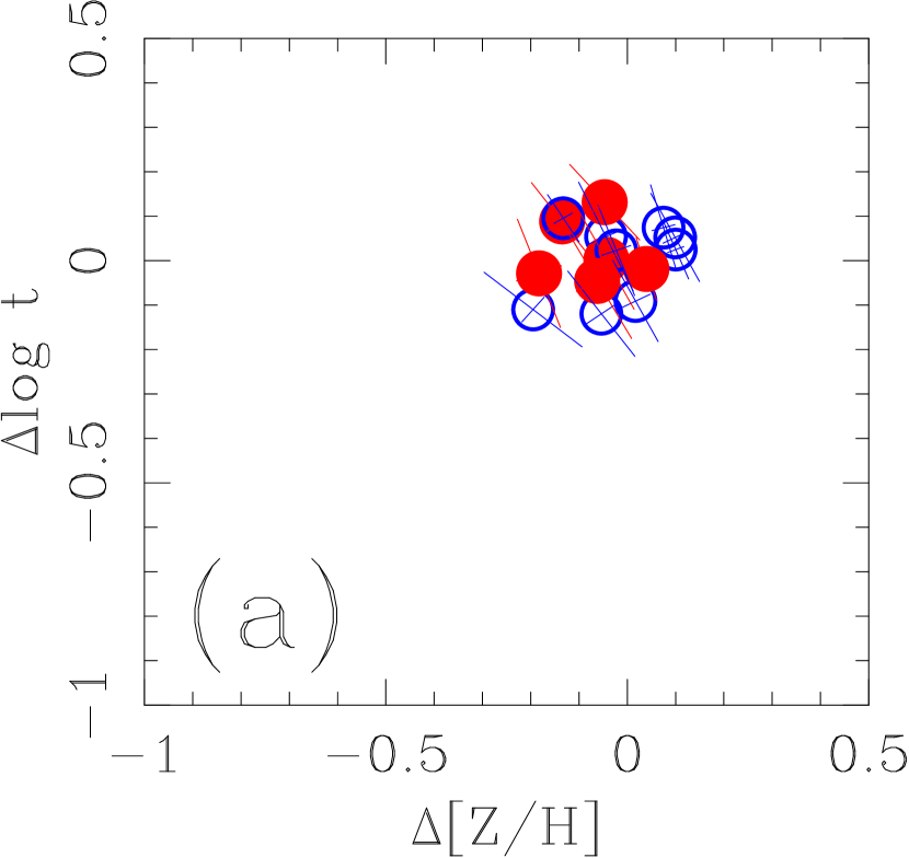
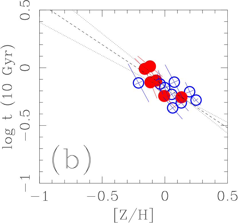
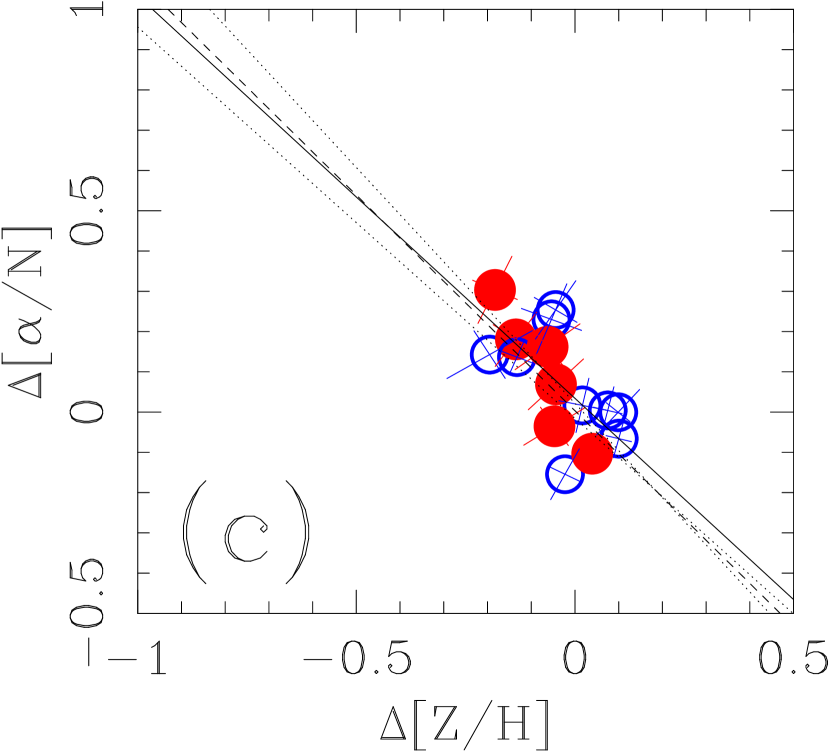
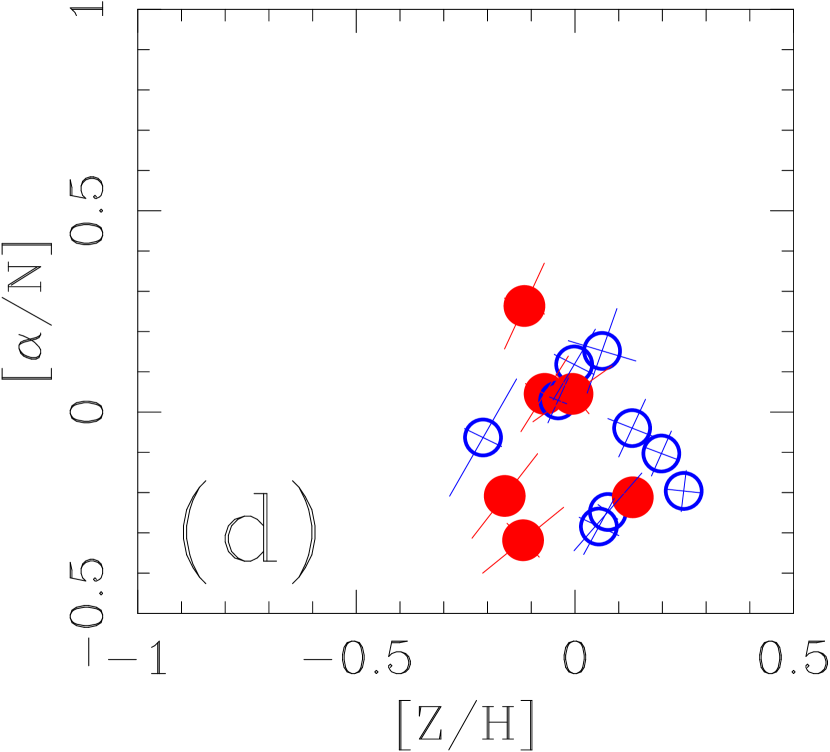
Figure 14.— The relative and absolute age-metallicity and nitrogen-metallicity diagrams for those E/S0 galaxies with $\sigma>134$ km/s. (a) and (c) show the results from the differential fitting. (b) and (d) show the parameters derived assuming no zero-point correction. When the models are not recalibrated to the data, the results are quite striking: (1) a “statistically” significant anti-correlation between $\log t$ and [Z/H] appears, with a slope of $-0.74\pm 0.13$ dex/dex (shown by the dashed and dotted lines); and (2) the nitrogen-metallicity correlation completely disappears, masking the true nature of the nitrogen enhancements. Systematic uncertainties in the calibrations of our indices would have obscured the true nature of early-type stellar populations. Note that the induced correlation between the absolute ages and metallicities obeys the famed “3/4” rule (Worthey, 1994).

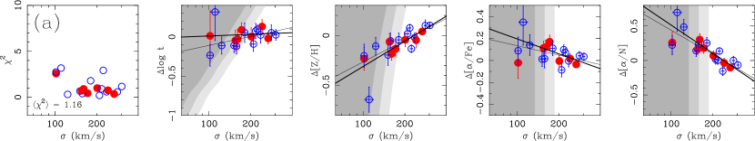
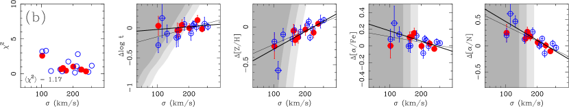
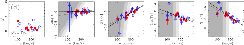
Figure 15.— The effects of varying the model zero-point on the relative stellar population parameters as functions of velocity dispersion. In (a), (b), (c), and (d) we show the results using the zero-points defined by Models 0, A, B, and C, respectively, defined in Table 5. Note that (a) is identical to Fig. 6(c). The general trends, and scatter about these trends, are insensitive to these large changes in the adopted zero-point. Because the variations in the recalibration probed here are much larger than the true uncertainties in the reference parameters, we conclude that our results are insensitive to systematic errors in the recalibration.

Table 1Corrected Velocity Dispersions and Balmer Line Strengths

ID	Type	$\log\sigma$	H$\delta_{A}$	H$\delta_{F}$	H$\gamma_{A}$	H$\gamma_{F}$	H$\beta$
095	S0	$2.321\pm 0.013$	$-1.37\pm 0.57$	$0.22\pm 0.17$	$-5.11\pm 0.30$	$-1.50\pm 0.17$	$1.72\pm 0.13$
135	S0	$2.180\pm 0.014$	$-0.35\pm 0.28$	$1.01\pm 0.18$	$-3.83\pm 0.27$	$-0.62\pm 0.16$	$2.43\pm 0.16$
182	S0	$2.091\pm 0.018$	$-0.35\pm 0.40$	$0.38\pm 0.27$	$-3.49\pm 0.40$	$-0.63\pm 0.23$	$1.87\pm 0.27$
211	S0	$2.257\pm 0.015$	$-0.97\pm 0.29$	$0.51\pm 0.19$	$-4.47\pm 0.31$	$-0.93\pm 0.19$	$2.21\pm 0.19$
212	E	$2.235\pm 0.014$	$-0.52\pm 0.28$	$0.52\pm 0.20$	$-4.41\pm 0.23$	$-0.70\pm 0.13$	$1.79\pm 0.13$
215	S0	$2.198\pm 0.015$	$-0.88\pm 0.38$	$0.50\pm 0.25$	$-4.41\pm 0.39$	$-1.09\pm 0.24$	$2.29\pm 0.21$
233	E/S0	$2.348\pm 0.008$	$-0.97\pm 0.17$	$0.92\pm 0.10$	$-4.60\pm 0.17$	$-0.88\pm 0.10$	$2.15\pm 0.09$
236	S0	$2.271\pm 0.012$	$\cdots$	$\cdots$	$-5.10\pm 0.37$	$-0.83\pm 0.18$	$1.86\pm 0.21$
242	E	$2.304\pm 0.011$	$-1.27\pm 0.22$	$0.51\pm 0.14$	$-4.97\pm 0.25$	$-1.44\pm 0.16$	$1.37\pm 0.14$
256	E	$2.395\pm 0.007$	$\cdots$	$0.43\pm 0.10$	$-4.85\pm 0.16$	$-1.14\pm 0.08$	$1.75\pm 0.08$
269	E/S0	$2.482\pm 0.008$	$-1.78\pm 0.16$	$0.21\pm 0.10$	$-5.45\pm 0.20$	$-1.37\pm 0.11$	$1.84\pm 0.08$
292	S0	$2.028\pm 0.012$	$\cdots$	$\cdots$	$-2.21\pm 0.25$	$0.66\pm 0.16$	$2.38\pm 0.16$
298	S0	$2.449\pm 0.008$	$-1.86\pm 0.19$	$0.51\pm 0.12$	$-5.29\pm 0.21$	$-1.39\pm 0.13$	$1.85\pm 0.09$
300	S0	$2.372\pm 0.010$	$-1.29\pm 0.21$	$0.61\pm 0.15$	$-5.21\pm 0.26$	$-1.50\pm 0.15$	$1.58\pm 0.13$
303	E	$2.191\pm 0.011$	$-0.55\pm 0.22$	$0.80\pm 0.13$	$-4.21\pm 0.26$	$-0.70\pm 0.15$	$1.94\pm 0.15$
309	E/S0	$2.336\pm 0.009$	$-1.31\pm 0.20$	$0.37\pm 0.13$	$-5.49\pm 0.24$	$-1.51\pm 0.14$	$1.69\pm 0.10$
353	E/S0	$2.336\pm 0.008$	$\cdots$	$\cdots$	$-5.18\pm 0.21$	$-1.41\pm 0.11$	$1.52\pm 0.09$
359	S0	$2.279\pm 0.010$	$\cdots$	$\cdots$	$-4.09\pm 0.25$	$-0.73\pm 0.15$	$1.92\pm 0.12$
360	E	$2.226\pm 0.048$	$\cdots$	$\cdots$	$-3.32\pm 0.97$	$-1.08\pm 0.63$	$1.52\pm 0.52$
375	E	$2.470\pm 0.010$	$\cdots$	$\cdots$	$-5.69\pm 0.35$	$-1.92\pm 0.30$	$1.54\pm 0.58$
381	E/S0	$2.304\pm 0.011$	$\cdots$	$\cdots$	$-4.54\pm 0.26$	$-0.95\pm 0.15$	$1.83\pm 0.15$
391	E/S0	$2.392\pm 0.011$	$\cdots$	$0.74\pm 0.23$	$-4.49\pm 0.21$	$-0.96\pm 0.13$	$1.83\pm 0.11$
408	S0	$2.352\pm 0.011$	$\cdots$	$0.80\pm 0.18$	$-4.77\pm 0.26$	$-1.10\pm 0.14$	$1.75\pm 0.11$
409	E	$2.008\pm 0.027$	$-0.85\pm 0.51$	$0.69\pm 0.29$	$-4.39\pm 0.58$	$-0.62\pm 0.34$	$2.39\pm 0.41$
410	S0	$2.149\pm 0.015$	$\cdots$	$\cdots$	$-4.71\pm 0.41$	$-0.99\pm 0.23$	$2.54\pm 0.23$
412	E	$2.206\pm 0.016$	$-0.30\pm 0.27$	$0.76\pm 0.18$	$-3.85\pm 0.27$	$-0.56\pm 0.18$	$1.52\pm 0.20$
463	S0	$2.431\pm 0.010$	$\cdots$	$\cdots$	$-4.52\pm 0.22$	$-0.97\pm 0.13$	$1.51\pm 0.14$
481	S0	$2.007\pm 0.022$	$-0.04\pm 0.42$	$1.73\pm 0.25$	$-2.03\pm 0.48$	$0.14\pm 0.32$	$2.47\pm 0.31$
493	E/S0	$2.043\pm 0.031$	$1.85\pm 0.57$	$1.99\pm 0.38$	$-4.38\pm 0.60$	$-0.94\pm 0.36$	$2.03\pm 0.44$
531	E	$2.426\pm 0.008$	$-1.68\pm 0.12$	$0.35\pm 0.09$	$-5.30\pm 0.17$	$-1.37\pm 0.09$	$1.77\pm 0.08$
534	E	$2.060\pm 0.022$	$\cdots$	$\cdots$	$-3.51\pm 0.43$	$-0.35\pm 0.26$	$2.00\pm 0.26$
536	E	$2.382\pm 0.009$	$-1.68\pm 0.20$	$0.56\pm 0.13$	$-5.28\pm 0.22$	$-1.45\pm 0.13$	$1.79\pm 0.10$

Table 2Corrected Molecular and Metal Line Strengths

ID	CN1	CN2	Ca4227Å	G4300Å	Fe4383Å	Ca4455Å	Fe4531Å	C4668Å	Fe5015Å	Mg$b$
095	$0.06\pm 0.01$	$0.08\pm 0.01$	$0.69\pm 0.34$	$5.11\pm 0.26$	$4.47\pm 0.32$	$1.04\pm 0.19$	$3.24\pm 0.25$	$6.02\pm 0.35$	$4.83\pm 0.34$	$4.27\pm 0.29$
135	$0.01\pm 0.01$	$0.04\pm 0.01$	$0.75\pm 0.15$	$5.02\pm 0.23$	$3.73\pm 0.39$	$1.00\pm 0.22$	$2.97\pm 0.28$	$3.95\pm 0.76$	$5.32\pm 0.38$	$\cdots$
182	$-0.03\pm 0.01$	$0.01\pm 0.01$	$1.09\pm 0.17$	$5.12\pm 0.36$	$2.87\pm 0.60$	$0.43\pm 0.34$	$2.81\pm 0.36$	$5.07\pm 0.57$	$2.88\pm 0.39$	$\cdots$
211	$0.03\pm 0.01$	$0.06\pm 0.01$	$1.27\pm 0.12$	$5.35\pm 0.28$	$4.05\pm 0.44$	$1.12\pm 0.36$	$2.57\pm 0.27$	$5.29\pm 0.55$	$4.48\pm 0.41$	$\cdots$
212	$0.03\pm 0.01$	$0.06\pm 0.01$	$0.91\pm 0.13$	$5.41\pm 0.21$	$2.98\pm 0.34$	$0.87\pm 0.20$	$2.65\pm 0.22$	$5.45\pm 0.53$	$4.29\pm 0.29$	$2.74\pm 0.38$
215	$0.02\pm 0.01$	$0.04\pm 0.01$	$0.78\pm 0.19$	$4.99\pm 0.33$	$3.30\pm 0.48$	$0.89\pm 0.27$	$3.07\pm 0.37$	$5.68\pm 0.47$	$4.38\pm 0.36$	$2.99\pm 0.43$
233	$0.03\pm 0.01$	$0.06\pm 0.01$	$0.87\pm 0.08$	$5.61\pm 0.13$	$3.88\pm 0.21$	$1.07\pm 0.11$	$3.34\pm 0.16$	$5.06\pm 0.26$	$4.58\pm 0.22$	$\cdots$
236	$0.04\pm 0.01$	$0.07\pm 0.01$	$0.96\pm 0.17$	$5.43\pm 0.26$	$4.27\pm 0.55$	$1.05\pm 0.21$	$3.39\pm 0.25$	$6.14\pm 0.51$	$4.64\pm 0.31$	$4.20\pm 0.30$
242	$0.05\pm 0.01$	$0.08\pm 0.01$	$1.06\pm 0.11$	$5.05\pm 0.20$	$4.01\pm 0.23$	$1.18\pm 0.15$	$2.87\pm 0.17$	$5.79\pm 0.77$	$4.48\pm 0.28$	$3.99\pm 0.26$
256	$0.06\pm 0.01$	$0.09\pm 0.01$	$1.08\pm 0.11$	$5.35\pm 0.14$	$4.24\pm 0.36$	$1.19\pm 0.29$	$3.31\pm 0.14$	$6.11\pm 0.27$	$4.83\pm 0.17$	$3.96\pm 0.29$
269	$0.10\pm 0.01$	$0.13\pm 0.01$	$1.09\pm 0.09$	$5.49\pm 0.14$	$4.43\pm 0.24$	$1.17\pm 0.11$	$3.00\pm 0.19$	$7.16\pm 0.24$	$4.85\pm 0.19$	$4.31\pm 0.24$
292	$\cdots$	$\cdots$	$0.76\pm 0.14$	$4.55\pm 0.21$	$3.38\pm 0.36$	$0.70\pm 0.27$	$2.86\pm 0.21$	$4.52\pm 0.39$	$4.67\pm 0.33$	$2.02\pm 0.28$
298	$0.08\pm 0.01$	$0.12\pm 0.01$	$1.24\pm 0.12$	$5.51\pm 0.16$	$4.33\pm 0.29$	$1.21\pm 0.12$	$3.41\pm 0.17$	$6.97\pm 0.81$	$5.45\pm 0.20$	$4.18\pm 0.40$
300	$0.07\pm 0.01$	$0.12\pm 0.01$	$0.92\pm 0.11$	$5.30\pm 0.21$	$4.34\pm 0.35$	$1.43\pm 0.37$	$3.15\pm 0.19$	$5.75\pm 0.36$	$5.03\pm 0.29$	$4.20\pm 0.27$
303	$0.04\pm 0.01$	$0.06\pm 0.01$	$0.92\pm 0.20$	$5.42\pm 0.20$	$3.90\pm 0.62$	$1.07\pm 0.32$	$3.12\pm 0.21$	$5.15\pm 0.70$	$4.80\pm 0.27$	$3.32\pm 0.37$
309	$0.08\pm 0.01$	$0.12\pm 0.01$	$0.97\pm 0.12$	$5.61\pm 0.19$	$3.75\pm 0.32$	$0.75\pm 0.25$	$3.27\pm 0.18$	$7.00\pm 0.32$	$5.04\pm 0.24$	$4.00\pm 0.27$
353	$\cdots$	$\cdots$	$0.75\pm 0.12$	$5.25\pm 0.16$	$3.95\pm 0.26$	$0.88\pm 0.16$	$3.06\pm 0.16$	$6.04\pm 0.31$	$4.43\pm 0.21$	$3.78\pm 0.20$
359	$\cdots$	$\cdots$	$0.85\pm 0.14$	$4.79\pm 0.21$	$3.73\pm 0.46$	$1.05\pm 0.32$	$3.25\pm 0.20$	$5.36\pm 0.39$	$3.84\pm 0.33$	$3.40\pm 0.32$
360	$\cdots$	$\cdots$	$-0.15\pm 0.66$	$4.10\pm 0.86$	$2.95\pm 1.61$	$1.13\pm 0.92$	$2.40\pm 0.75$	$2.44\pm 1.20$	$8.18\pm 0.89$	$4.36\pm 0.72$
375	$0.12\pm 0.01$	$0.15\pm 0.01$	$0.95\pm 0.10$	$5.40\pm 0.15$	$4.37\pm 0.26$	$1.19\pm 0.09$	$3.48\pm 0.14$	$6.82\pm 0.27$	$5.50\pm 0.41$	$4.45\pm 0.37$
381	$0.04\pm 0.03$	$0.07\pm 0.02$	$0.91\pm 0.12$	$5.15\pm 0.27$	$4.02\pm 0.29$	$0.99\pm 0.18$	$2.98\pm 0.22$	$5.00\pm 0.50$	$4.31\pm 0.34$	$3.87\pm 0.29$
391	$0.05\pm 0.01$	$0.08\pm 0.01$	$1.22\pm 0.14$	$5.07\pm 0.18$	$4.00\pm 0.32$	$1.02\pm 0.24$	$3.15\pm 0.19$	$5.41\pm 0.48$	$4.50\pm 0.36$	$3.54\pm 0.43$
408	$0.03\pm 0.01$	$0.06\pm 0.01$	$0.46\pm 0.33$	$5.66\pm 0.23$	$3.94\pm 0.32$	$1.10\pm 0.28$	$3.19\pm 0.20$	$6.20\pm 0.34$	$4.18\pm 0.33$	$3.66\pm 0.39$
409	$-0.01\pm 0.01$	$0.02\pm 0.02$	$0.76\pm 0.32$	$4.88\pm 0.53$	$2.55\pm 0.68$	$0.71\pm 0.40$	$4.19\pm 0.46$	$4.07\pm 0.92$	$3.57\pm 0.75$	$4.24\pm 0.70$
410	$\cdots$	$\cdots$	$1.08\pm 0.21$	$5.18\pm 0.36$	$3.62\pm 0.48$	$1.21\pm 0.29$	$3.93\pm 0.34$	$6.75\pm 0.52$	$4.35\pm 0.41$	$4.28\pm 0.75$
412	$0.01\pm 0.01$	$0.03\pm 0.01$	$1.19\pm 0.40$	$5.32\pm 0.24$	$3.30\pm 0.32$	$0.95\pm 0.27$	$2.57\pm 0.23$	$4.42\pm 0.52$	$4.38\pm 0.39$	$3.35\pm 0.24$
463	$\cdots$	$\cdots$	$1.02\pm 0.11$	$5.10\pm 0.18$	$4.16\pm 0.28$	$1.09\pm 0.17$	$3.31\pm 0.19$	$6.20\pm 0.75$	$4.46\pm 0.24$	$3.99\pm 0.30$
481	$-0.01\pm 0.01$	$0.03\pm 0.01$	$1.23\pm 0.23$	$4.49\pm 0.42$	$2.53\pm 0.71$	$1.14\pm 0.39$	$2.87\pm 0.42$	$3.66\pm 0.75$	$4.64\pm 0.60$	$3.47\pm 0.45$
493	$-0.07\pm 0.02$	$-0.04\pm 0.02$	$0.44\pm 0.34$	$5.41\pm 0.56$	$2.28\pm 0.94$	$1.39\pm 0.55$	$3.06\pm 0.59$	$0.88\pm 1.14$	$3.99\pm 0.74$	$3.59\pm 1.07$
531	$0.08\pm 0.00$	$0.12\pm 0.00$	$0.99\pm 0.09$	$5.33\pm 0.14$	$4.54\pm 0.18$	$1.16\pm 0.09$	$3.15\pm 0.14$	$6.35\pm 0.22$	$4.63\pm 0.20$	$4.37\pm 0.23$
534	$\cdots$	$\cdots$	$\cdots$	$4.15\pm 0.35$	$3.07\pm 1.72$	$\cdots$	$2.60\pm 0.38$	$3.80\pm 0.92$	$1.93\pm 0.85$	$\cdots$
536	$0.07\pm 0.01$	$0.10\pm 0.01$	$1.11\pm 0.11$	$5.30\pm 0.17$	$3.99\pm 0.29$	$1.16\pm 0.13$	$3.06\pm 0.16$	$6.04\pm 0.77$	$4.74\pm 0.23$	$3.88\pm 0.28$

Table 3First Partial Derivatives of the Models

$X$	$\partial X\over\partial\log t$	$\partial X\over\partial[{\rm Z/H}]$	$\partial X\over\partial[\alpha{\rm/Fe}]$	$\partial X\over\partial[\alpha/{\rm N}]$	$\partial X\over\partial[\alpha/{\rm C}]$	$\partial X\over\partial[\alpha/{\rm Ca}]$
H$\delta_{F}$	$-1.813$	$-1.356$	$2.064$	$\ldots$	$\ldots$	$\ldots$
H$\delta_{A}$	$-4.299$	$-4.185$	$4.743$	$\ldots$	$\ldots$	$\ldots$
CN1	$0.122$	$0.198$	$0.058$	$-0.147$	$-0.474$	$\ldots$
CN2	$0.126$	$0.213$	$0.066$	$-0.164$	$-0.507$	$\ldots$
Ca4227	$1.000$	$1.444$	$-0.034$	$0.421$	$2.259$	$-1.767$
G4300	$1.462$	$1.748$	$1.584$	$\ldots$	$-4.779$	$\ldots$
H$\gamma_{F}$	$-2.612$	$-2.232$	$1.181$	$\ldots$	$\ldots$	$\ldots$
H$\gamma_{A}$	$-4.229$	$-4.637$	$3.788$	$\ldots$	$\ldots$	$\ldots$
Fe4383	$2.156$	$4.920$	$-4.488$	$\ldots$	$\ldots$	$\ldots$
Ca4455	$0.693$	$1.434$	$0.104$	$\ldots$	$\ldots$	$\ldots$
Fe4531	$0.973$	$2.084$	$-1.013$	$\ldots$	$\ldots$	$\ldots$
C4668	$2.142$	$8.953$	$1.209$	$\ldots$	$-50.216$	$\ldots$
H$\beta$	$-1.154$	$-0.629$	$0.289$	$\ldots$	$\ldots$	$\ldots$
Fe5015	$1.001$	$3.208$	$-1.574$	$\ldots$	$\ldots$	$\ldots$
Mg$b$	$1.761$	$3.183$	$2.123$	$\ldots$	$\ldots$	$\ldots$

Note. — The partial derivatives given above are computed by adding 0.3 dex to the adopted reference parameters $\{\log t,[{\rm Z/H}],[\alpha{\rm/Fe}],[\alpha/{\rm N}],[\alpha/{\rm C}],[\alpha/{\rm Ca}]\}=\{-0.15,0.3,0.2,0,0,0\}$. Note that we define age in units of $10^{10}$ yr, and thus the reference age is equivalent to $t=7$ Gyr, or a redshift of formation of $z_{f}=2.4$ (Kelson et al., 2001). Thus $\partial X/\partial p\equiv\Delta X/0.3$, where $p\in\{\log t,[{\rm Z/H}],[\alpha{\rm/Fe}],[\alpha/{\rm N}],[\alpha/{\rm C}],[\alpha/{\rm Ca}]\}$. Where the partial derivatives are not given, and assumed to be identically zero, Thomas, Maraston, & Bender (2003a) and Thomas, Maraston, & Korn (2004) had either reported, qualitatively, that the index was insensitive to changes in the relevant parameter, or the model cannot contain information on the sensitivity of the index to the parameter because they did not (or could not) include it in their analyses. This fact helps to underscore the importance of zero-pointing the model to a fiducial observed dataset as it removes the importance of such unknown/undefined dependences to zeroth order. The Thomas, Maraston, & Bender (2003a) and Thomas, Maraston, & Korn (2004) set of predictions is highly non-linear such that at other locations in the 6D parameter domain these derivatives are not valid. As a result, the above partial derivatives should only illustrate a broad sensitivity of the indices to changes in the model parameters.

Table 4The Zero-point Offsets for Recalibrating the Models to the Data

$X$	$X_{\rm model}$	$X_{\rm\langle CL1358\rangle}$	$\Delta_{X}$	units
H$\delta_{F}$	$0.261$	$0.519$	$0.258$	Å
H$\delta_{A}$	$-2.109$	$-1.468$	$0.641$	Å
CN1	$0.080$	$0.060$	$-0.020$	mag
CN2	$0.113$	$0.094$	$-0.020$	mag
Ca4227	$1.432$	$0.958$	$-0.474$	Å
G4300	$6.042$	$5.326$	$-0.716$	Å
H$\gamma_{F}$	$-1.461$	$-1.265$	$0.196$	Å
H$\gamma_{A}$	$-5.829$	$-5.004$	$0.825$	Å
Fe4383	$5.496$	$4.138$	$-1.358$	Å
Ca4455	$1.945$	$1.096$	$-0.848$	Å
Fe4531	$3.573$	$3.166$	$-0.407$	Å
C4668	$7.228$	$6.074$	$-1.154$	Å
H$\beta$	$1.755$	$1.729$	$-0.025$	Å
Fe5015	$5.855$	$4.690$	$-1.165$	Å
Mg$b$	$4.422$	$4.000$	$-0.422$	Å

Note. — The model values given above are computed at the adopted reference parameters $\{\log t,[{\rm Z/H}],[\alpha{\rm/Fe}],[\alpha/{\rm N}],[\alpha/{\rm C}],[\alpha/{\rm Ca}]\}=\{-0.15,0.3,0.2,0,0,0\}$. Note that we define age in units of $10^{10}$ yr, and thus the reference age is equivalent to $t=7$ Gyr, or a redshift of formation of $z_{f}=2.4$ (Kelson et al., 2001).

Table 5Tested Variations in the Zero-point of the Models

Model	$\log[t/(10\hbox{ Gyr})]$	[Z/H]	[$\alpha$/Fe]	[$\alpha$/N]	[$\alpha$/C]	[$\alpha$/Ca]
0a	$-0.15$	$0.30$	$0.20$	$0.00$	$0.00$	$0.00$
A	$\,\,\ 0.00$	$0.30$	$0.30$	$0.00$	$0.00$	$0.00$
B	$-0.15$	$0.30$	$0.00$	$0.00$	$0.00$	$0.00$
C	$-0.15$	$0.00$	$0.00$	$0.00$	$0.00$	$0.00$

Note. — ^aThe zero-point used in the analysis presented in the paper.

References

- Aoki & Tsuji (1997) Aoki, W., & Tsuji, T. 1997, A&A, 328, 175
- Barr et al. (2005) Barr, J., Davies, R., Jørgensen, I., Bergmann, M., & Crampton, D. 2005, AJ, 130, 445
- Baum (1959) Baum, W. A. 1959, PASP, 71, 106
- Beers, Flynn, & Gebhardt (1990) Beers, T. C., Flynn, K., & Gebhardt, K. 1990, AJ, 100, 32
- Bellman et al. (2001) Bellman, S., Briley, M. M., Smith, G. H., & Claver, C. F. 2001, PASP, 113, 326
- Bensby, Feltzing, & Lundström (2004) Bensby, T., Feltzing, S., & Lundström, I. 2004, A&A, 415, 155
- Blakeslee et al. (2006) Blakeslee, J. P., et al. 2006, ApJ, 644, 30
- Boothroyd & Sackmann (1999) Boothroyd, A. I., & Sackmann, I.-J. 1999, ApJ, 510, 232
- Bower, Lucey, & Ellis (1992) Bower, R.G., Lucey, J.R., & Ellis, R.S. 1992, MNRAS, 254, 601
- Briley, Cohen, & Stetson (2002) Briley, M. M., Cohen, J. G., & Stetson, P. B. 2002, ApJ, 579, L17
- Briley, Cohen, & Stetson (2004a) Briley, M. M., Cohen, J. G., & Stetson, P. B. 2004a, AJ, 127, 1579
- Briley et al. (2004b) Briley, M. M., Harbeck, D., Smith, G. H., & Grebel, E. K. 2004b, AJ, 127, 1588
- Bruzual & Charlot (2003) Bruzual, G. & Charlot, S. 2003, MNRAS, 344, 1000
- Burbidge, Burbidge, & Fish (1961) Burbidge, E. M., Burbidge, G. R., & Fish, R. A. 1961, ApJ, 133, 393
- Burke (1968) Burke, J. A. 1968, MNRAS, 140, 241
- Burstein et al. (1984) Burstein, D., Faber, S. M., Gaskell, C. M., & Krumm, N. 1984, ApJ, 287, 586
- Burstein, Faber, & Gonzalez (1986) Burstein, D., Faber, S. M., & Gonzalez, J. J. 1986, AJ, 91, 1130
- Caldwell & Rose (1997) Caldwell, N., & Rose, J. A. 1997, AJ, 113, 492
- Caldwell, Rose, & Concannon (2003) Caldwell, N., Rose, J. A., & Concannon, K. D. 2003, AJ, 125, 2891
- Cardiel et al. (1998) Cardiel, N., Gorgas, J., Cenarro, J, & González, J.J. 1998, A&AS, 127, 597
- Cardiel et al. (2003) Cardiel, N., Gorgas, J., Sánchez-Blázquez, P., Cenarro, A. J., Pedraz, S., Bruzual, G., & Klement, J. 2003, A&A, 409, 511
- Carretero et al. (2004) Carretero, C., Vazdekis, A., Beckman, J. E., Sánchez-Blázquez, P., & Gorgas, J. 2004, ApJ, 609, L45
- Cenarro et al. (2003) Cenarro, A. J., Gorgas, J., Vazdekis, A., Cardiel, N., & Peletier, R. F. 2003, MNRAS, 339, L12
- Cenarro et al. (2004) Cenarro, A. J., Sánchez-Blázquez, P., Cardiel, N., & Gorgas, J. 2004, ApJ, 614, L101
- Charbonnel (1994) Charbonnel, C. 1994, A&A, 282, 811
- Djorgovski & Davis (1987) Djorgovski S., & Davis M. 1987, ApJ, 313, 59
- Dressler et al. (1987) Dressler, A., Lynden-Bell, D., Burstein, D., Davies, R.L., Faber, S.M, Terlevich, R.J. & Wegner, G 1987, ApJ, 313, 42
- Dressler et al. (1997) Dressler, A., Oemler, A., Jr., Couch, W. J., Smail, I., Ellis, R. S., Barger, A., Butcher, H., Poggianti, B. M., & Sharples, R. M. 1997, ApJ, 490, 577
- Faber (1972) Faber, S. M. 1972, A&A, 20, 361
- Faber & Jackson (1976) Faber, S.M. & Jackson, R.E. 1976, ApJ, 204, 668
- Faber et al. (1985) Faber, S. M., Friel, E.D., Burstein, D., & Gaskell, C. M., 1985, ApJS, 57, 711
- Fabricant, Franx, & van Dokkum (2000) Fabricant, D., Franx, M., & van Dokkum, P. 2000, ApJ, 539, 577
- Falcón-Barroso et al. (2003) Falcón-Barroso, J., Peletier, R. F., Vazdekis, A., & Balcells, M. 2003, ApJ, 588, L17
- Fisher, Franx, & Illingworth (1996) Fisher, D., Franx, M., & Illingworth, G. 1996, ApJ, 459, 110
- Fisher et al. (1998) Fisher, D., Fabricant, D., Franx, M., & van Dokkum P.G. 1998, ApJ, 498, 195
- Franx, Illingworth, & Heckman (1989) Franx M., Illingworth, G., & Heckman, T. 1989, AJ, 98, 538
- Gallazzi et al. (2005) Gallazzi, A., Charlot, S., Brinchmann, J., White, S. D. M., & Tremonti, C. A. 2005, MNRAS, 362, 41
- Garbow, Hillstrom, & More (1980) Garbow, B.S., Hillstrom, K.E., & More, J.J., 1980, http://www.netlib.org/minpack/
- González (1993) González, J.J. 1993, Ph.D. thesis, Univ. Calif., Santa Cruz
- Gorgas et al. (1993) Gorgas, J., Faber, S. M., Burstein, D., González, J. J., Courteau, S., & Prosser, C. 1993, ApJS, 86, 153
- Gratton, Sneden, & Caretta (2004) Gratton, R., Sneden, C., & Carretta, E. 2004, ARA&A, 42, 385
- Henry & Worthey (1999) Henry, R. B. C. & Worthey, G. 1999, PASP, 111, 919
- Henry, Edmunds, & Köppen (2000) Henry, R. B. C., Edmunds, M. G., & Köppen, J. 2000, ApJ, 541, 660
- Holden et al. (2004) Holden, B. P., Stanford, S. A., Eisenhardt, P., & Dickinson, M. 2004, AJ, 127, 2484
- Holden et al. (2005) Holden, B. P., et al. 2005, ApJ, 620, L83
- Holden et al. (2006) Holden, B. P., et al. 2006, ApJ, 642, L123
- Jørgensen, Franx, & Kjærgaard (1995) Jørgensen I., Franx M., & Kjærgaard P. 1995, MNRAS, 276, 1341
- Jørgensen (1997) Jørgensen, I. 1997, MNRAS, 288, 161
- Jørgensen (1999) Jørgensen, I. 1999, MNRAS, 306, 607
- Jørgensen et al. (2005) Jørgensen, I., Bergmann, M., Davies, R., Barr, J., Takamiya, M., & Crampton, D. 2005, AJ, 129, 1249
- Jørgensen et al. (2006) Jørgensen, I., Chiboucas, K., Flint, K., Bergmann, M., Barr, J., & Davies, R. 2006, ApJ, 639, L9
- Juneau et al. (2005) Juneau, S., et al. 2005, ApJ, 619, L135
- Kauffmann et al. (1993) Kauffmann, G., White, S. D. M., & Guiderdoni, B. 1993, MNRAS, 264, 201
- Kauffmann et al. (1999) Kauffmann, G., Colberg, J. M., Diaferio, A., & White, S. D. M. 1999, MNRAS, 303, 188
- Kaviraj et al. (2005) Kaviraj, S., Devriendt, J. E. G., Ferreras, I., & Yi, S. K. 2005, MNRAS, 360, 60
- Kelson et al. (1997) Kelson, D.D., van Dokkum, P.G., Franx, M., Illingworth, G.D., & Fabricant, D. 1997, ApJ, 478, L13
- Kelson et al. (2000a) Kelson, D.D., Illingworth, G.D., van Dokkum, P.G., & Franx, M. 2000a, ApJ, 531, 137
- Kelson et al. (2000b) Kelson, D.D., Illingworth, G.D., van Dokkum, P.G., & Franx, M. 2000b, ApJ, 531, 159
- Kelson et al. (2000c) Kelson, D.D., Illingworth, G.D., van Dokkum, P.G., & Franx, M. 2000c, ApJ, 531, 184
- Kelson et al. (2001) Kelson, D. D., Illingworth, G. D., Franx, M., & van Dokkum, P. G. 2001, ApJ, 552, L17
- Kelson et al. (2006a) Kelson, D.D., et al. 2006a, in prep
- Kelson et al. (2006b) Kelson, D.D., et al. 2006b, in prep
- Köppen & Edmunds (1999) Köppen, J., & Edmunds, M. G. 1999, MNRAS, 306, 317
- Köppen & Hensler (2005) Köppen, J., & Hensler, G. 2005, A&A, 434, 531
- Korn, Maraston, & Thomas (2005) Korn, A. J., Maraston, C., & Thomas, D. 2005, A&A, 438, 685
- Kuntschner (1998) Kuntschner, H. 1998, Ph.D. Thesis, University of Durham, United Kingdom
- Kuntschner (2000) Kuntschner, H. 2000, MNRAS, 315, 184
- Kuntschner et al. (2001) Kuntschner, H., Lucey, J. R., Smith, R. J., Hudson, M. J., & Davies, R. L. 2001, MNRAS, 323, 615
- Lanzoni et al. (2005) Lanzoni, B., Guiderdoni, B., Mamon, G. A., Devriendt, J., & Hatton, S. 2005, MNRAS, 361, 369
- Marigo et al. (1998) Marigo, P., Bressan, A., & Chiosi, C. 1998, A&A, 331, 564
- Mehlert et al. (2003) Mehlert, D., Thomas, D., Saglia, R. P., Bender, R., & Wegner, G. 2003, A&A, 407, 423
- Michielsen et al. (2003) Michielsen, D., De Rijcke, S., Dejonghe, H., Zeilinger, W. W., & Hau, G. K. T. 2003, ApJ, 597, L21
- Minkowski (1962) Minkowski, R. 1962, IAU Symp. 15: Problems of Extra-Galactic Research, 15, 112
- Moran et al. (2005) Moran, S. M., Ellis, R. S., Treu, T., Smail, I., Dressler, A., Coil, A. L., & Smith, G. P. 2005, ApJ, 634, 977
- Morgan & Mayall (1957) Morgan, W. W., & Mayall, N. U. 1957, PASP, 69, 291
- Nelan et al. (2005) Nelan, J. E., Smith, R. J., Hudson, M. J., Wegner, G. A., Lucey, J. R., Moore, S. A. W., Quinney, S. J., & Suntzeff, N. B. 2005, ApJ, 632, 137
- Oke et al. (1995) Oke, J.B., et al. 1995, PASP, 107, 375
- Poggianti et al. (2001) Poggianti, B. M., et al. 2001, ApJ, 562, 689
- Postman et al. (2005) Postman, M., et al. 2005, ApJ, 623, 721
- Proctor et al. (2004a) Proctor, R. N., Forbes, D. A., Hau, G. K. T., Beasley, M. A., De Silva, G. M., Contreras, R., & Terlevich, A. I. 2004a, MNRAS, 349, 1381
- Proctor et al. (2004) Proctor, R. N., Forbes, D. A., & Beasley, M. A. 2004b, MNRAS, 355, 1327
- Rix & White (1992) Rix, H.-W. & White, S.D.M. 1992, MNRAS, 254, 389
- Romeo et al. (2005) Romeo, A. D., Portinari, L., & Sommer-Larsen, J. 2005, MNRAS, 361, 983
- Rood (1969) Rood, H. J. 1969, ApJ, 158, 657
- Saglia et al. (1993) Saglia, R. P., Bertschinger, E., Baggley, G., Burstein, D., Colless, M., Davies, R. L., McMahan, R. K., & Wegner, G. 1993, MNRAS, 264, 961
- Saglia et al. (2002) Saglia, R. P., Maraston, C., Thomas, D., Bender, R., & Colless, M. 2002, ApJ, 579, L13
- Sánchez-Blázquez (2004) Sánchez-Blázquez, P. 2004, Ph.D. Thesis, Universidad Complutense de Madrid, Spain
- Schiavon et al. (2002) Schiavon, T.P., Faber, S.M., Castilho, B.V., & Rose, J. A. 2002, ApJ, 580, 850
- Schiavon, Caldwell, & Rose (2004) Schiavon, R. P., Caldwell, N., & Rose, J. A. 2004, AJ, 127, 1513
- Schiavon (2005) Schiavon, R. P., 2005, ApJS, submitted
- Stanford, Eisenhardt, & Dickinson (1998) Stanford, S.A., Eisenhardt, P.R., & Dickinson, M. 1998, ApJ, 492, 461
- Terlevich et al. (1981) Terlevich, R., Davies, R.L., Faber, S.M. & Burstein, D. 1981, MNRAS, 196, 381
- Thomas, Maraston, & Bender (2003a) Thomas, D., Maraston, C., & Bender, R. 2003a, MNRAS, 339, 897
- Thomas, Maraston, & Bender (2003b) Thomas, D., Maraston, C., & Bender, R. 2003b, MNRAS, 343, 279
- Thomas, Maraston, & Korn (2004) Thomas, D., Maraston, C., & Korn, A. 2004, MNRAS, 351, L19
- Thomas et al. (2005) Thomas, D., Maraston, C., Bender, R., & de Oliveira, C. M. 2005, ApJ, 621, 673
- Tonry & Davis (1979) Tonry, J. & Davis, M. 1979, AJ, 84, 1511
- Trager et al. (1998) Trager, S.C., Worthey, G., Faber, S.M., Burstein, D., González, J.J. 1998, ApJS, 116, 1
- Trager et al. (2000a) Trager, S.C., Faber, S.M., Worthey, G., & González, J.J.2000a, AJ, 119, 1645
- Trager et al. (2000b) Trager, S.C., Faber, S.M., González, J.J., & Worthey, G. 2000b, AJ, 120, 165
- Trager (2002) Trager, S.C., 2002, private communication
- Tran et al. (2005) Tran, K.-V. H., van Dokkum, P., Franx, M., Illingworth, G. D., Kelson, D. D., & Schreiber, N. M. F. 2005, ApJ, 627, L25
- Tripicco & Bell (1995) Tripicco, M.J. & Bell, R.A. 1995, AJ, 110, 3035
- van Dokkum et al. (1998a) van Dokkum, P. G., Franx, M., Kelson, D. D., Illingworth, G. D., Fisher, D., & Fabricant, D. 1998a, ApJ, 500, 714
- van Dokkum et al. (1998b) van Dokkum, P. G., Franx, M., Kelson, D. D., and Illingworth, G. D., 1998b, ApJ, 504, L17
- van Dokkum & Stanford (2003) van Dokkum, P. G., & Stanford, S. A. 2003, ApJ, 585, 78
- Vazdekis (1999) Vazdekis, A. 1999, ApJ, 513, 224
- Vazdekis et al. (1996) Vazdekis, A., Casuso, E., Peletier, R.F., Beckman, J.E. 1996, ApJS, 106, 307
- Worthey (1994) Worthey, G. 1994, ApJS, 95, 107
- Worthey et al. (1994) Worthey, G., Faber, S. M., Gonzalez, J. J., & Burstein, D. 1994, ApJS, 94, 687
- Worthey & Ottaviani (1997) Worthey, G. & Ottavianni, D.L. 1997, ApJS, 111, 377
- Worthey (1998) Worthey, G. 1998, PASP, 110, 888
- Worthey & Collobert (2003) Worthey, G. & Collobert, M. 2003, ApJ, 586, 17
- Wuyts et al. (2004) Wuyts, S., van Dokkum, P.G., Kelson, D.D., Franx, M., & Illingworth, G.D. 2004, ApJ, 605, 677
- Ziegler & Bender (1997) Ziegler, B. L., & Bender, R. 1997, MNRAS, 291, 527
- Ziegler et al. (2005) Ziegler, B. L., Thomas, D., Böhm, A., Bender, R., Fritz, A., & Maraston, C. 2005, A&A, 433, 519