Numerical Simulations of the Lyman-$\alpha$ forest – A comparison of Gadget-2 and Enzo

Abstract

We compare simulations of the Lyman-$\alpha$ forest performed with two different hydrodynamical codes, Gadget-2 and Enzo. A comparison of the dark matter power spectrum for simulations run with identical initial conditions show differences of 1-3% at the scales relevant for quantitative studies of the Lyman-$\alpha$ forest. This allows a meaningful comparison of the effect of the different implementations of the hydrodynamic part of the two codes. Using the same cooling and heating algorithm in both codes the differences in the temperature and the density probability distribution function are of the order of 10 %. The differences are comparable to the effects of boxsize and resolution on these statistics. When self-converged results for each code are taken into account the differences in the flux power spectrum – the statistics most widely used for estimating the matter power spectrum and cosmological parameters from Lyman-$\alpha$ forest data – are about 5%. This is again comparable to the effects of boxsize and resolution. Numerical uncertainties due to a particular implementation of solving the hydrodynamic or gravitational equations appear therefore to contribute only moderately to the error budget in estimates of the flux power spectrum from numerical simulations. We further find that the differences in the flux power spectrum for Enzo simulations run with and without adaptive mesh refinement are also of order 5% or smaller. The latter require 10 times less CPU time making the CPU time requirement similar to that of a version of Gadget-2 that is optimised for Lyman-$\alpha$ forest simulations.

1 Introduction

There is now a well established paradigm for the origin of the Lyman-$\alpha$ forest, the ubiquitous absorption lines due to neutral hydrogen in the spectra of high-redshift quasars. The absorption blue-wards of 1216 $\AA$ is predominantly due to density fluctuations in the intervening warm ($\sim 10^{4}$ K) photoionized inter-galactic medium (IGM) on scales larger than the Jeans length of the gas (see Rauch (1998) for a review). Numerical simulations were instrumental in establishing the new paradigm in the 1990s (Cen et al. (1994), Zhang et al. (1995), Hernquist et al. (1996), Theuns et al. (1998), Zhang et al. (1997)). The Lyman-$\alpha$ forest and the associated metal absorption probe the thermal and ionization history of the IGM as well as the interplay of galaxies and the IGM from which they are formed. More recently the Lyman-$\alpha$ forest has also been established as a means of quantitative measurement of the underlying matter distribution and thus a variety of cosmological parameters (e.g. Croft et al. (1998), Croft et al. (2002), Viel et al. (2004), Seljak et al. (2005), Viel & Haehnelt (2006), Seljak et al. (2006); Viel, Haehnelt & Lewis (2006)). Numerical simulations thereby play a crucial role in inferring the linear matter power spectrum and other derived quantities from the Lyman-$\alpha$ forest data. With increasing sample sizes statistical errors of measurements of the flux distributions have reached the percent level and the error budget is dominated by systematic uncertainties (Viel, Haehnelt & Springel (2004), McDonald et al. (2005) ). Uncertainties due to numerical simulations contribute significantly to the error budget and the accuracy with which the flux distribution for given input physics and cosmological parameters can be simulated has become important. Most studies so far have used convergence tests to assess uncertainties due to the numerical simulations and direct comparisons of cosmological hydrodynamical simulation performed with different codes have been rare. The differences between hydro-dynamical simulations of galaxy clusters with a wide range of different codes/methods have been studied in the Santa Barbara cluster project (Frenk et al. 1999). Recently O’Shea et al. (2005) performed a comparison between the grid based adaptive mesh refinement (AMR) code Enzo and the smoothed particle hydrodynamics (SPH) code Gadget-2. However, little has been done in this respect for hydrodynamical simulations of the Lyman-$\alpha$ forest data (see Theuns et al. (1998) for a notable exception of a comparison between two SPH codes) Some comparisons of hydrodynamical simulations with approximate simulations of the Lyman-$\alpha$ forest data have been performed by McDonald et al. (2005),Zhan et al. (2005) and Viel, Haehnelt & Springel (2006). We present here a comparison of hydrodynamical simulations of the Lyman-$\alpha$ forest with Enzo and Gadget-2 which concentrates on the statistical properties of the flux distribution.
We are therefore mostly interested in properties of the moderate to low over-density gas which is responsible for Lyman-$\alpha$ forest absorption. Of particular interest is the probability distribution of the gas density, the temperature, the resulting flux distribution and the flux power spectrum. A major difference between grid-based and SPH codes is their treatment of shocks and their effects on the temperature distribution. We will also examine these differences.
The plan of the paper is as follows. In §2 we describe the Enzo code and the Gadget-2 code and the different ways in which the codes solve the gravitational and hydrodynamics equations. In §2.4 we describe the simulation set used in the comparisons. In §3 we investigate how physical properties of both codes compare, in particular the gas distribution and the 1-D flux power spectrum. Finally in §3.3 we will look at the performance of each code in terms of CPU time consumption.

2 Hydrodynamical simulations of the Lyman-$\alpha$ forest

2.1 Grid-based simulations vs. SPH simulations

The physical state of the gas responsible for the Lyman-$\alpha$ forest is largely governed by the competing processes of photoionisation and adiabatic cooling due to expansion. The low over-density gas obeys a tight temperature - density relation, (e.g. Katz et al. (1996), Hui & Gnedin (1997) ) which can be approximated by

$$T=T_{0}\Big{(}{\rho_{b}\over\overline{\rho}_{b}}\Big{)}^{\gamma-1}$$ (1)

where $\rho_{b}$ and $\overline{\rho}_{b}$ are the baryon density and mean baryon density respectively, $T$ is the temperature, $T_{0}$ and $1<\gamma<1.6$ are parameters which depend on the reionisation history model and the spectral shape of the UV background. Typical temperatures of the photoionized IGM are in the range 10000-20000 K. The optical depth for Lyman-$\alpha$ absorption is proportional to the neutral hydrogen density, (Gunn & Peterson, 1965), which, since the gas is in photoionisation equilibrium, is proportional to the square of the density times the recombination rate,

$$\tau\propto\Big{(}{\rho_{b}\over\overline{\rho}_{b}}\Big{)}^{2}T^{-0.7}=A\Big{(}{\rho_{b}\over\overline{\rho}_{b}}\Big{)}^{\beta}$$ (2)

where $\beta=2.7-0.7\gamma$. The factor A depends on the redshift, baryon density, temperature at the mean density, Hubble constant and the photoionisation rate. The optical depth is a faithful tracer of the matter distribution on scales larger than the Jeans length of the photoionized IGM. Even though the density field is only mildly non-linear on the relevant scales the thermal effects, the peculiar velocities and the non-linear relation between flux and optical depth make hydrodynamical simulations mandatory for accurate predictions of the statistical properties of the flux distribution in the Lyman-$\alpha$ forest. Cosmological hydrodynamical simulations come in two basic flavours, SPH (Lucy 1977, Gingold & Monaghan 1977) and grid based codes. SPH codes like Gadget-2 use particles to represent the baryonic fluid. SPH is a Lagrangian method and hence the resolution is concentrated in regions of high density. Grid based codes like Enzo, use a grid of cells to represent the gas properties. One of the options in Enzo is an adaptive refinement of the grid where the grid resolution is increased in regions of high density resulting in a large dynamic range. Both codes have been used to study the Lyman-$\alpha$ forest (e.g Viel, Haehnelt & Springel (2004), Tytler et al. (2004), Bolton et al. (2005), Jena et al. (2005), McDonald et al. (2005)). SPH simulations of the Lyman-$\alpha$ forest in particular have been very successful but in principle one may think that a grid based code could offer better resolution of the low density IGM than SPH codes because in SPH simulations the resolution in low density regions decreases when the gravitational clustering of the matter distribution becomes non-linear and high density regions start to form. Grid-based codes could also offer a more accurate treatment of shocks which are relevant for the thermal state of the IGM. We will now briefly describe the methods implemented in Enzo and Gadget-2 to solve the gravitational and hydrodynamical equations.

Particle number/Rootgridsize	Boxsize ($h^{-1}$ Mpc)	SDR
Enzo AMR Grid
$50^{3}$	15.0      30.0      60.0	800
$100^{3}$	15.0      30.0      60.0	1600
$200^{3}$	15.0      30.0      60.0	3200
Enzo Static Grid
$50^{3}$	15.0      30.0      60.0	50
$100^{3}$	15.0      30.0      60.0	100
$200^{3}$	15.0      30.0      60.0	200
$400^{3}$	15.0      30.0      60.0	400
Gadget-2
$50^{3}$	15.0      30.0      60.0	800
$100^{3}$	15.0        30.0       60.0	1600
$200^{3}$	15.0       30.0      60.0	3200
Gadget-2 (star formation)
$400^{3}$	15.0       30.0      60.0	6400

Table 1: Spatial parameters and spatial dynamic range (SDR) for the Enzo AMR simulations, the Enzo static grid simulations and the Gadget-2 simulations with and without star formation. The particle numbers for Gadget-2 and the rootgridsize for Enzo is shown in the left hand column. In the Gadget-2 simulations the number of DM particles and SPH particles is equal and for the Enzo simulations the number of DM particles is equal to the rootgridsize.

2.2 Enzo 

Enzo is a Eulerian adaptive mesh refinement code originally developed by Greg Bryan and Mike Norman at the University of Illinois (Bryan & Norman 1995b, Bryan & Norman 1997, Norman & Bryan 1999, O’Shea et al. 2004). The hydrodynamics solver employs the Piecewise Parabolic method combined with a non-linear Riemann solver for shock capturing. The Eulerian AMR scheme was first developed by Berger & Oliger (1984) and later refined by Berger & Colella (1989) to solve the hydrodynamical equations for an ideal gas. Bryan & Norman 1997 adopted such a scheme for cosmological simulations. The gravity solver in Enzo uses a N-Body particle mesh technique (Efstathiou et al. 1985, Hockney & Eastwood 1988).
We have used the publicly available version of Enzo (Enzo -1.0.1) which we have modified to use the Gadget-2 equilibrium chemistry solver as discussed in §2.2.2.

2.2.1 Enzo gravity solver

The gravity solver in Enzo employs an adaptive particle-mesh algorithm. The potential is solved on a periodic root grid using Fast Fourier Transforms. In order to accurately account for the sub grids a multi-grid relaxation technique is used (see e.g. Norman & Bryan 1999). The force resolution is typically twice as coarse as the grid resolution.

Figure 1: Left Panel: Top: The DM power spectrum of the Enzo AMR simulations with a rootgridsize of $200^{3}$. The arrows indicate the Nyquist frequency for the rootgrid for the 60 $h^{-1}$ Mpc , 30 $h^{-1}$ Mpc and 15 $h^{-1}$ Mpc boxes (comoving) from left to right. Bottom: The fractional difference between the Enzo simulations with and without AMR [(Enzo(AMR) - Enzo(static) ) / Enzo(AMR) ]. Right Panel: The fractional difference between the DM power spectrum of simulations with Gadget-2 and Enzo(AMR) [(Gadget-2 - Enzo(AMR) ) / Gadget-2 ]. All results are for $z=3.0$.

2.2.2 Enzo hydrodynamics solver

Enzo uses the Piecewise parabolic method (PPM), (Woodward & Colella, 1984) for solving the hydrodynamic equations. A complete description of this method is not possible here and we will only give short description (see Bryan et al. (1995) for more details). PPM is a higher order accurate version of Godunov’s method with a third order accurate piecewise parabolic monotonic interpolation and a non-linear Riemann solver for shock capturing. The method is second order accurate in space and time and explicitly conserves energy mass flux and momentum. It uses a dual energy formalism which allows the calculation of both the thermal energy and the total energy of the gas at each time step. This ensures a correct internal energy and the correct entropy jump at shock fronts and the correct temperature and pressure in hypersonic flows. This represents a major difference with respect to SPH codes which employ an artificial viscosity to capture shocks (see Springel & Hernquist (2002)).
In addition to solving the ideal gas dynamics Enzo also has several cooling and heating routines. For the cooling both non-equilibrium and equilibrium cooling functions are available.

We will use here a modified version of Enzo, which, uses the Gadget-2 equilibrium chemistry solver for hydrogen and helium with a uniform ultra-violet(UV) background based on the models of Haardt & Madau (1996).

2.2.3 The adaptive mesh refinement

The AMR ability of Enzo introduces finer and finer grids into areas of high density thus allowing maximum resolution where it is actually needed at a minimum computational expense. This ability to dynamically refine the resolution is essential for accurately tracking the non-linear collapse of rapidly evolving density fields. For Lyman-$\alpha$ forest simulations the resolution in high density regions is less important and we investigate here simulations with and without AMR. With AMR the hydrodynamical equations are initially solved on a uniform grid, the solutions are monitored and the patches of the initially uniform grid are refined if certain refinement criteria are met. Parent grids then produce child grids. For cosmological studies a refinement factor of 2 is normally used. This means that a child grid will have cells which have twice the spatial resolution of the parent grid. It is also worth noting that grids at the same level will have the same timestep but that this timestep may be different for grids at a different level of refinement. For Lyman-$\alpha$ forest simulations it is not obvious how important the use of the AMR option is. Most of the absorption especially at high redshift is by gas of moderate (over)density. Note that previous studies of the Lyman-$\alpha$ forest with grid-based codes have generally not used AMR methods (e.g. Jena et al. 2005, McDonald et al. 2005). However as shown by Viel et al. (2004) the few strong absorption systems caused by dense regions contribute significantly to the flux power spectrum at all scales. We will investigate this further in §3.2.4.

2.3 Gadget-2 

Gadget-2 (Springel 2005), the updated version of Gadget-1 (Springel 2001) is a parallel TreePM-SPH code. On the scales relevant for the Lyman-$\alpha$ forest Gadget-2 in its TREEPM mode is similar to a PM code with some extra resolution due to the Tree part of the algorithm on small and intermediate scales. The gravitational components of Gadget-2 and Enzo are therefore somewhat similar on large scales most relevant for the Lyman-$\alpha$ forest. The hydrodynamical components are, however, very different.
We have used a version of Gadget-2 which is similar to the publicly available version as of August 2006. The only exceptions are that we have used a Gadget-2 equilibrium cooling algorithm supplied to us by the authors of Gadget-2 , and that some of the simulations discussed in sections §2.4 and §3.2.4, were run with a version of Gadget-2 optimised for speed for Lyman-$\alpha$ forest simulations where gas with an overdensity $>$ 1000 and a temperature $<$ $10^{5}$ K is turned into collisionless star particles (see Viel et al. 2004 for more details).

2.3.1 The Gadget-2 gravity solver

We have used a version of Gadget-2 which employs a TreePM algorithm to solve the gravitational equations (Xu 1995, Bode et al. 2000, Bagla & Ray 2003). The TreePM algorithm is a hybrid of the tree (Barnes & Hut, 1986) and particle mesh methods (Efstathiou et al. 1985, Hockney & Eastwood 1988). It utilises the best elements of both making the gravitational force determination more accurate and efficient. The potential is split into two components $\phi_{k}=\phi^{\rm long}_{k}+\phi^{\rm short}_{k}$, where

$$\phi^{\rm long}_{k}=\phi_{k}exp(-k^{2}r^{2}_{s})$$ (3)

and $r_{s}$ is the spatial scale of the force split which is usually set to a little larger than the mesh spacing. For the simulations performed here we used the Gadget-2 default value of $r_{s}$ equal to 1.25 times the mesh spacing and a mesh spacing equal to the cube root of the total number of dark matter particles. The long range force is then computed using mesh methods making the long range force almost exact. The short range force is computed using a tree algorithm which calculates the gravitational particle-particle forces on small and intermediate scales in an efficient manner.
In order to conserve the symplectic nature of the leap-frog time integration for the case of individual timesteps the Hamiltonian is separated into a kinetic part and a long range and short range potential. Gadget-2 then evolves all particles using individual timesteps hence reducing the computational overhead that would be associated with evolving all the particles using the minimum allowed timestep. The splitting of the time integration is similar to what is done in the TreePM algorithm (see Springel 2005 for more details). TreePM codes offer an excellent compromise between speed and accuracy.

2.3.2 The Gadget-2 Hydrodynamics solver

The Gadget-2 hydrodynamics solver uses the SPH formalism. SPH can be thought of as a discretisation of a fluid which is then represented by particles. Continuous fluid properties are then defined using kernel interpolation. The particles sample the gas in a Lagrangian sense thus making SPH methods very powerful for following structure formation in cosmological simulations.
The thermodynamic state of each fluid element can either be defined in terms of its thermal energy per unit mass, $u_{i}$, or its entropy per unit mass, $s_{i}$. In Gadget-2 the entropy per unit mass, $s_{i}$, is used (see Springel & Hernquist(2002)). The code conserves both energy and entropy even when fully adaptive smoothing lengths are used. This represents a major change in methods between Gadget-1 and Gadget-2 which is investigated in O’Shea et al. (2005).
A potential drawback of SPH is the approximate way in which it captures shocks by use of an artificial viscosity (see Springel (2005) for more details).
The large differences in the methodology of the hydro-solvers make a comparison of Lyman-$\alpha$ forest simulation with both codes very interesting for a test of the sensitivity of these simulations to a particular numerical method.

Figure 2: Left Panel: A comparison of the Enzo(AMR only) and Gadget-2 gas temperature over-density relation at $z=3$ for the $(15,200)$ simulations. The diamonds represent the Enzo simulation while pluses represent the Gadget-2 simulation. 10000 values from each simulation are plotted. Right Panel: PDF of the volume-weighted gas temperature distribution for the $(15,200)$ simulations with Enzo with and without AMR and Gadget-2 with and without simplified star formation. All the results are at $z=3.0$.

2.4 Simulation parameters

We have performed simulations with parameters of the concordance cosmological model with $\Omega_{\Lambda}=0.74,\Omega_{\rm m}=0.26,\Omega_{\rm b}=0.0463,\sigma_{8}=0.85,n=0.95$ and $h$ = 0.72. These simulation parameters correspond to the ’B2’ model of Viel et al. (2004). Identical initial conditions were used for the simulations with both codes. Enzo was run with the implementation of the Gadget-2 equilibrium chemistry so that cooling and heating were also treated in the same way. Theuns et al. (1998), Viel et al. (2004), McDonald et al. (2005), Jena et al. (2005) and Bolton et al. (2005) have investigated the effect of box size and resolution of hydrodynamical simulations on a variety of statistics of the Lyman-$\alpha$ forest flux distribution most importantly the flux probability distribution, the effective optical depth and the flux power spectrum. Unfortunately it is currently not possible to run hydrodynamical simulations for which these statistics are fully converged especially not for a large parameter space. Convergence and box size studies are therefore essential for quantitative studies of the Lyman-$\alpha$ forest. Generally compromises have to be made and the application of corrections and an analysis of the corresponding errors are necessary. Our aim is here to investigate how the uncertainties between codes employing different hydrodynamical methods compare to other errors in a quantitative analysis. We have thus ran simulations with up to four different numbers of basic resolution elements (number of particles and grid cells, respectively) and for three different box sizes. The Enzo simulations were run without AMR and with up to 4 levels of grid refinement. We have chosen a refinement level of 4 so as to match Spatial Dynamic Range (SDR) of SPH calculations currently used in calculating the flux statistics of the Lyman-$\alpha$ forest. The simulation parameters are summarised in Table 1. Note that only the higher resolution simulations resolve the Jeans mass well. We will come back to this later.
The SPH nature of the Gadget-2 simulations leads to a varying resolution similar to that of an AMR code. In order to get a feel for how the resolution of the different simulations compare, the last column of Table 1 gives the SDR. For the SPH simulation the SDR is calculated as ${\rm SDR}$ = L/$\epsilon$ where $\epsilon$ is the gravitational softening length and is calculated before the simulation begins by dividing the boxsize L by the number of particles along one axis times some constant factor.
The Enzo simulations were run with a static grid and with AMR. For Enzo the SDR is calculated as ${\rm SDR}={N_{\rm root}\times 2^{l}}$, where $N_{\rm root}$, is the size of the root grid in 1D and $l$ is the refinement factor. In the static grid simulations the grids are fixed throughout the simulation without any refinement. As a result the spatial resolution in high density regions will be comparatively poor in these simulations. Most of the absorption in the Lyman-$\alpha$ forest is, however, produced by regions of low or moderate density. As we will see later the differences in the statistics of the flux distribution between simulations with and without AMR are therefore actually moderate. The static grid simulations would be comparable in resolution to a Gadget-2 simulation with a softening length equal to the mean inter-particle spacing.
Unfortunately the improved resolution of the AMR simulations comes at the expense of a significant increase in computational time. For the AMR simulations we set the maximum refinement level to 4 beyond which an artificial pressure support is introduced to prevent further collapse. We thereby experimented with the values of the parameters for the minimum pressure support and checked that the thermodyamic properties of the cells in question were not affected. The mesh-refinement criterion was set to the standard values of 4 for the dark matter (DM) and 8 for the baryons (see O’Shea et al. (2005) for more details). This means that a grid will refine when its DM density reaches a factor 4 greater than the root DM density or when its baryonic density reaches a factor of 8 greater than the root baryonic density. To make contact with the simulations used in actual measurements of the matter power spectrum from Lyman-$\alpha$ forest data we also investigated some of the simulations used in Viel et al. (2004). These simulations employ a simplified star formation criterion that turns all gas with an over-density, with respect to the mean baryonic density, $>1000$ and temperature $<10^{5}$ K into collisionless star particles. This substantially reduces the required computational time by eliminating the short dynamic time scales associated with high density gas and significantly speeds up Lyman-$\alpha$ forest simulations with Gadget-2. The effect on the statistics of the flux distribution has been shown to be small (see Viel et al. (2004)) and we have labelled these simulations as Gadget-2 (stars).
Most of these simulations have very large particle numbers ($2\times 400^{3}$). Unfortunately for these simulations only a comparison with the Enzo static grid simulations is feasible with our limited computational resources.

Figure 3: PDF of the volume-weighted gas density distribution for simulations with Enzo with and without AMR and Gadget-2 with and without simplified star formation. The panels are for simulations with a boxsize of $15h^{-1}$,$30h^{-1}$ and $60h^{-1}$ Mpc (comoving) from left to right. All the results are at $z=3.0$.

We will concentrate our comparison on simulation outputs at $z=3$ the centre of the redshift range $2<z<4$ relevant for quantitative measurements of the matter power spectrum studies from Lyman-$\alpha$ forest data, but will briefly discuss simulations of the Lyman-$\alpha$ flux power spectrum at $z=2$ and $z=4$ in §3.2.4.

Figure 4: PDF of the flux distribution for simulations with Enzo with and without AMR and Gadget-2 with and without simplified star formation. The panels are for simulations with a boxsize of $15h^{-1}$,$30h^{-1}$ and $60h^{-1}$ Mpc (comoving) from left to right with $200^{3}$ particles/rootgridsize. The bottom panel shows the fractional differences between the Enzo(AMR) simulation and the Gadget-2 simulation (solid curve), the Enzo(AMR) and Enzo(static) simulations(dotted curve) and between the Gadget-2 simulations with and without star formation (dashed curve in the left panel) All the results are at $z=3.0$.

3 Code Comparisons

3.1 The dark matter distribution

We start with a comparison of the DM distribution. O’Shea et al. (2005) have recently performed such a comparison and found moderate differences but note that we are interested in a different application of the code than investigated in O’Shea et al. (2005). The most relevant statistical property of the matter distribution is the power spectrum $P(k)=<|\delta_{k}|^{2}>$, where $\delta_{k}$ is the Fourier transform of the density field. O’Shea found very good agreement at large scales with deviations at small scales.
The left panel of Figure 1 shows the DM power spectrum of the Enzo(AMR) simulation in the form $\Delta^{2}(k)=P(k)k^{3}$ for three simulations with a $200^{3}$ root grid but different box sizes at $z=3$. The bottom panel in the left panel of Figure 1 shows the percentage difference between simulations with and without AMR in the form [(Enzo(AMR) - Enzo(static) ) / Enzo(AMR) ]. As expected the AMR simulations show more small scale power as the particle mesh algorithm becomes more accurate at small scales due to mesh refinement. The differences at large scales are very small, of the order of $1\%$. In the right panel of Figure 1 we have plotted the fractional difference between the DM power spectrum of the Enzo(AMR) and the Gadget-2 simulations in the form [(Gadget-2 - Enzo(AMR) )/Gadget-2 ]. Similar to O’Shea we find differences of $\sim 1\%$ at large scales.
The strong increase at small scales is due to the somewhat different resolution limits of the simulations compared. O’Shea et al. (2005) came to a similar conclusion and showed that Enzo and Gadget-2 produce very similar results, even at small scales, when a low over-density threshold is used for the mesh-refinement criteria. As pointed out by O’Shea et al. (2005), and verified by us, Gadget-2 has a higher force resolution and hence more power at small scales due to the better force resolution of the Tree algorithm when simulations of similar SDR are compared and standard parameters are used in both simulations. Note, however, that for simulations of the Lyman-$\alpha$ forest the differences at the relevant scales are very small. This makes a meaningful comparison of the effect of the different hydrodynamics solvers on the statistics of the flux distribution – the main aim of this paper – possible.

3.2 Properties of the gas distribution

3.2.1 Shock heating and the thermal state of the gas

As we described in §2 at moderate to low over densities ($\delta\lesssim 5$) the temperature - density relation is well approximated by a power law. In the left panel of Figure 2 we have plotted the temperature - density relation for a simulation with 2 $\times 200^{3}$ DM and gas particles/rootgridsize in a $15h^{-1}$ Mpc box, hereafter labelled as a ($15,200$) simulation, for Enzo(AMR) and Gadget-2. 10000 points are plotted for each simulation. This gives a feel for the level of shock heating produced by each code and also emphasises that the vast majority of the gas lies very close to a line representing the power law approximation. The temperature is volume-weighted in both cases. We have chosen volume-weighted temperatures as the flux statistics of the Lyman-$\alpha$ forest are volume-weighted. Temperatures and densities were calculated in the same way as for the mock absorption spectra. Note that the differences for the mass-weighted temperatures were somewhat smaller.
Overall the agreement between the two codes is remarkable given the very different ways in which both codes treat shocks. As mentioned previously Gadget-2 uses a conservative entropy formalism to treat shocks while Enzo uses a non-linear Riemann solver. In principle since Gadget-2 employs an artificial viscosity to capture shocks Enzo should resolve shocks more accurately and one may have expected that weak shocks may occur in low density regions which Gadget-2 does not capture properly. This appears not to be the case. The amount of shock heated gas and its temperature distribution is very similar. This can be seen more clearly in the right panel of Figure 2 where we have plotted the volume weighted probability distribution function (PDF) of the temperature for simulations with Enzo with and without AMR and for Gadget-2 with and without the simplified star formation criterion. The differences are of order 10% and can be at least partially attributed to differences in the PDF of the density which we will discuss in the next section.

3.2.2 The probability distribution function of the gas density

Figure 3 shows the volume-weighted PDF of the gas distribution for simulations with a range of box sizes. The agreement between the Enzo simulations with and without AMR in this linear volume-weighted plot which emphasises gas around the mean density is very good. The differences between the simulations with Gadget-2 and Enzo are somewhat larger, of order 10%. Note, however, that this is smaller than the differences due to changes in box size and resolution. Overall the agreement is again very good.

As demonstrated in the previous sections, a SPH code and a grid-based code differ in their resolution properties and it is not trivial to run simulations with the “same resolution” because of differences in force resolution and the way the resolution is distributed between regions of different densities. The (small) differences between simulations with Enzo and Gadget-2 are thus not surprising.

3.2.3 The probability distribution of the flux

We have computed the flux distribution for 1000 random lines of sight through the simulation box. The optical depth has been rescaled in the standard way to match the observed effective optical depth at $z=3$ as given by Schaye et al. (2003), $\tau_{\rm eff}=0.363$. Figure 4 shows the corresponding probability distribution of the flux for simulations with Enzo with and without AMR and Gadget-2 with and without simplified star formation. Overall the flux distributions are very similar. Typical differences between the simulations with Enzo and Gadget-2 are 5-10%. The differences are again smaller than those due to changes of box size and resolution. The differences between the Gadget-2 simulations with and without star formation are less than 3%.

Figure 5: The top panel shows the flux power spectrum for simulations with Enzo(AMR) with a boxsize of $15h^{-1}$,$30h^{-1}$,$60h^{-1}$ Mpc comoving. The middle panel shows fractional differences between the Enzo simulation with and without AMR [Enzo(AMR) - Enzo(static) )/Enzo(AMR) ]. The top and middle panel are for $z=3$ and the line styles are identical. The bottom panel shows the effect of resolution on the flux power spectrum at $z=2$. The differences are relative to the highest resolution run e.g. ((15, 400) - (15,200)) / (15,400).

3.2.4 The flux power spectrum

In Figure 5, we show the flux power spectrum for the Enzo AMR simulations for different boxsizes at $z=3$. The middle panel shows the fractional difference between Enzo simulations with and without AMR. The solid curve is for simulations with a boxsize 15 $h^{-1}$ Mpc, the dashed curve is for a boxsize of 30 $h^{-1}$ Mpc box and the dotted curve is for a box size of 60 $h^{-1}$ Mpc. At large scales the differences are less than 4%. At the resolution limit the differences increase as expected. The effect of the AMR is most significant at small scales. Note that the force resolution limit (twice the cell length) is about an order of magnitude off the graph on the right hand side. The bottom panel of Figure 5 demonstrates the convergence of the flux power spectrum by comparing the flux power spectrum for the static grid simulations with a box size of 15 $h^{-1}$ Mpc at $z=2$. The differences between the (15,200) and (15,400) simulations are less than 2 percent on the relevant scales suggesting that a resolution of 150$h^{-1}$ kpc (comoving) is required to reach convergence. This is in good agreement with the results by Viel et al. (2004) for the Gadget-2 simulations also used here. Note, however, that a similar comparison by Jena et al. (2005) for static grid Enzo simulations with the same resolution as shown in the bottom panel (their Figure 7) showed significantly larger differences. A discrepant result for which we do not have an explanation.

We have also investigated how the level of AMR refinement effects the Lyman-$\alpha$ flux power spectrum. The results for simulations with refinement level 2 lie in between those with refinement level 4 shown in Figure 5 and the static grid simulations. This suggests that a relatively high refinement level may be needed to correctly account for the effect of strong absorption systems on the flux power spectrum caused by high density gas which Viel et al. (2004) have shown to extend to large scales.

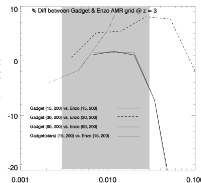
Figure 6: The fractional difference of the flux power spectrum of simulations with Enzo(AMR) and Gadget-2 for different box sizes [(Gadget-2 - Enzo(AMR))/Gadget-2 ]. Also shown is the difference for Gadget-2 simulations with and without star formation. The shaded region indicates the range of wave numbers used by Viel et al. (2004) to infer the linear dark matter power spectrum.

In Figure 6 we show the fractional difference of the flux power spectrum of the Gadget-2 and Enzo simulations for the $200^{3}$ simulations. Apart from the smallest scales in the lowest resolution simulation the differences are about 5%. The differences are scale dependent and appear to decrease with increased resolution. Unfortunately we did not have the computational resources available to run Enzo(AMR) simulation with a root-grid size of $400^{3}$. In Figure 7 we therefore show the differences between $400^{3}$ Gadget-2 and Enzo(static) simulations. The differences are again about 5%. The reader should thereby keep in mind the differences of up to 4% between the Enzo(AMR) and Enzo(static) simulations. Note that Viel et al. (2004) found the (60,400) simulations to be the best compromise between box size and resolution in their measurement of the matter power spectrum from Lyman-$\alpha$ forest data. We have also looked into the differences at $z=2$ and $z=4$ and found the differences to be redshift dependent. At $z=4$ the differences are similar than those at $z=3$ while at $z=2$ they are somewhat larger. By investigating the $z=3$ simulations with different effective optical depth we verified that the change of the differences of the simulated flux power spectra with redshift is mainly but not only due to the strong evolution of the effective optical depth. Also worth noting is the excellent agreement between the Gadget-2 simulation with (thin solid curve) and without star formation (thick solid curve) shown in Figure 6.

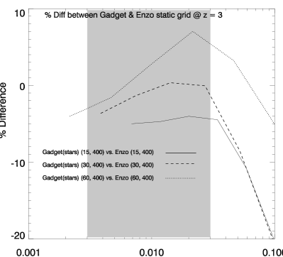
Figure 7: The fractional difference of the flux power spectrum of simulations with Enzo(static) and Gadget-2 for $400^{3}$ gas particle/rootgridsize simulations with different box sizes. The difference is of the form [(Gadget-2 - Enzo(static))/Gadget-2 ]. All Gadget simulations are in this case run with the simplified star formation algorithm. The shaded region indicates the range of wave numbers used by Viel et al. (2004) to infer the linear dark matter power spectrum.

3.3 CPU time requirements

We have performed a series of timing tests for both Enzo and Gadget-2 for a selection of the simulations used in this study. For the timings, simulations were carried out on the distributed memory Sun Cluster at the Institute of Astronomy in Cambridge and Cosmos a shared memory machine located at the Department of Applied Mathematics and Theoretical Physics (DAMTP) in Cambridge. On the distributed memory machine the timing tests were performed on 32 single node 500 Mhz processors with 2 Gbytes of memory and a 100 Mbit ethernet connect. The latency of the connection is approximately 300 microseconds. Although these processors are relatively slow by today’s standards they should still provide an illustration of the relative performance of the codes in different configurations. The tests were performed for simulations with a boxsize of 15 $h^{-1}$ Mpc comoving for particle (rootgridsize) numbers $50^{3}$, $100^{3}$, $200^{3}$. The results are shown in Figure 8. We ran the Enzo simulations for 10 time steps starting at $z=3.5$. For Gadget-2 we ran the simulation from $z=3.5$ to the same redshift that Enzo had reached. The Enzo(AMR) simulations are about a factor 1.5-2 faster than the Gadget-2 simulations without star formation. Turning the AMR off leads to a speed-up of a factor five for the Enzo simulations. The Gadget-2 simulations without star formation spends most of its time calculating the hydrodynamics of the very high density gas, which for the Lyman-$\alpha$ forest is not necessary. Turning on the star formation in Gadget-2 leads to a speed-up by a factor 30. As we have demonstrated here (see also Viel et al. (2004) ) the effect of turning on star formation in Gadget-2 on the statistics of the flux distribution is very small.
Cosmos is an SGI Altix 3700 with 152 Itanium2 (Madison) processors and 152GB of globally shared main memory. Each Madison processor has a clock speed of 1.3GHz, a 3MB L3 cache and a peak performance of 5.2 Gflops. The system is built from 76 dual-processor nodes, each with 2GB of local shared memory. These are linked by the SGI NUMAflexIII interconnects, which provides a high speed (3.2GB/sec bi-directional), low latency (sub-microsecond) network with a dual-plane, fat tree topology, connecting all processors with each other and with a single, globally shared and cache-coherent 152GB memory subsystem. We have only tested the two faster versions of the codes on the shared memory machine. The results are shown in Figure 8. Note the reversal in relative speed between Gadget-2 simulations with star formation and Enzo static grid simulation between the two architectures. Obviously Enzo benefits more strongly from the shared memory architecture (see O’Shea et al. (2005) for a similar result). The Enzo(static) simulation run about a factor three faster on the shared memory machine than the Gadget-2 simulations with star formation. Reducing the refinement level in the AMR simulation may thus offer a good compromise between accuracy and speed for Lyman-$\alpha$ forest simulations with Enzo .

4 Discussion and conclusions

We have performed a detailed comparison of Lyman-$\alpha$ forest simulations with Gadget-2 , a TreePM-SPH code, and Enzo a Eulerian AMR code in order to asses the numerical uncertainties due to a particular numerical implementation of solving the hydrodynamical equations. The codes are similar with respect to the way in which they compute the gravitational forces at large scales but differ in the way they calculate gravitational forces on small scales; the codes use a Tree-PM and PM N-body algorithm, respectively. Their main differences lie, however, in the way in which they solve the gas hydrodynamics. Gadget-2 discretises mass using SPH methods while Enzo discretises space using adaptive meshes. The main results are as follows.

• The differences in the dark matter power spectrum between simulations with Enzo and Gadget-2 on scales relevant for measurements of the matter power spectrum from Lyman-$\alpha$ forest data are about 2% for an appropriate choice of box size and resolution.

• The temperature density relation of simulations with Enzo and Gadget-2 differ very little. The PDF of the volume weighted temperature differ by $\sim 10$ % probably mainly due to differences in the PDF of the gas density which are of the same order and at least partially caused by a slight mismatch in resolution.

• The PDF of the flux distribution of simulations with Enzo and Gadget-2 agree very well. Typical differences are $\sim 5-10$% probably again mainly due to a slight mismatch of the resolution.

• The differences of the flux power spectrum of simulations with Enzo and Gadget-2 on scales relevant for measurements of the matter power spectrum from Lyman-$\alpha$ forest data are about 5% for an appropriate choice of box size and resolution and simulations which fully resolve the Jeans mass. For simulations of lower resolution but larger boxsize the difference increase up to $\sim 10$%. Note that the differences are scale and redshift dependent.

Figure 8: A comparison of the CPU time required for the simulation to run through a fixed redshift interval. Simulation parameters are as described in the text and annotated on the plot. The thin lines are for a SUN distributed memory cluster and the thick lines are for a SGI shared memory (SM) machine. Only relative values for the same architecture should be considered. Note the reversal in relative speed between Gadget-2 simulations with star formation and Enzo static grid simulation between the two architectures. The thick dashed line shows a linear scaling of CPU time with the number of particles for comparison.

Overall the Lyman-$\alpha$ forest simulations with Enzo and Gadget-2 agree astonishingly well. The choice of method for solving the hydrodynamical simulations appears to affect the gas distribution and its thermal state very little. It is also reassuring that two different implementations for solving the gravitational equations agree well. The corresponding uncertainties should contribute to the overall error budget of measurements of the matter power spectrum from Lyman-$\alpha$ forest data at the level of 3%. The total error in current measurement is significantly larger and they should thus not be important. The main numerical uncertainties are instead due to a lack of sufficient dynamic range which typically makes correction of 5% for boxsize and resolution necessary. This will obviously improve as computational resources become more powerful. In practical terms memory requirements of simulations with Enzo without AMR and Gadget-2 are similar. Enzo without AMR offers the highest speed but requires somewhat larger corrections. Our results suggest that if sufficient computational resources are available and sufficient care is employed the accuracy of numerical simulations should not yet be a limiting factor in improving the accuracy of measurements of the matter power spectrum from Lyman-$\alpha$ forest data.

References

- Bagla & Ray (2003) Bagla J. S., Ray S., 2003, New Astronomy, 8, 665
- Barnes & Hut (1986) Barnes J., Hut P., 1986, Nature, 324, 446
- Berger & Colella (1989) Berger M. J., Colella P., 1989, Journal of Computational Physics, 82, 64
- Berger & Oliger (1984) Berger M. J., Oliger J., 1984, Journal of Computational Physics, 53, 484
- Bode et al. (2000) Bode P., Ostriker J. P., Xu G., 2000, ApJS, 128, 561
- Bolton et al. (2005) Bolton J. S., Haehnelt M. G., Viel M., Springel V., 2005, MNRAS, 357, 1178
- Bryan & Norman (1995) Bryan G. L., Norman M. L., 1995, Bulletin of the American Astronomical Society, 27, 1421
- Bryan & Norman (1997) Bryan G. L., Norman M. L., 1997, in ASP Conf. Ser. 123: Computational Astrophysics; 12th Kingston Meeting on Theoretical Astrophysics Simulating X-Ray Clusters with Adaptive Mesh Refinement. pp 363–+
- Bryan et al. (1995) Bryan G. L., Norman M. L., Stone J. M., Cen R., Ostriker J. P., 1995, Computer Physics Communications, 89, 149
- Cen et al. (1994) Cen R., Miralda-Escude J., Ostriker J. P., Rauch M., 1994, ApJ, 437, L9
- Croft et al. (2002) Croft R. A. C., Weinberg D. H., Bolte M., Burles S., Hernquist L., Katz N., Kirkman D., Tytler D., 2002, ApJ, 581, 20
- Croft et al. (1998) Croft R. A. C., Weinberg D. H., Katz N., Hernquist L., 1998, ApJ, 495, 44
- Efstathiou et al. (1985) Efstathiou G., Davis M., White S. D. M., Frenk C. S., 1985, ApJS, 57, 241
- Frenk & et al (1999) Frenk C. S., et al 1999, ApJ, 525, 554
- Gingold & Monaghan (1977) Gingold R. A., Monaghan J. J., 1977, MNRAS, 181, 375
- Gunn & Peterson (1965) Gunn J. E., Peterson B. A., 1965, ApJ, 142, 1633
- Haardt & Madau (1996) Haardt F., Madau P., 1996, ApJ, 461, 20
- Hernquist et al. (1996) Hernquist L., Katz N., Weinberg D. H., Miralda-Escudé J., 1996, ApJ, 457, L51+
- Hockney & Eastwood (1988) Hockney R. W., Eastwood J. W., 1988, Computer simulation using particles. Bristol: Hilger, 1988
- Hui & Gnedin (1997) Hui L., Gnedin N. Y., 1997, MNRAS, 292, 27
- Jena et al. (2005) Jena T., Norman M. L., Tytler D., Kirkman D., Suzuki N., Chapman A., Melis C., Paschos P., O’Shea B., So G., Lubin D., Lin W.-C., Reimers D., Janknecht E., Fechner C., 2005, MNRAS, 361, 70
- Katz et al. (1996) Katz N., Weinberg D. H., Hernquist L., 1996, ApJS, 105, 19
- Lucy (1977) Lucy L. B., 1977, AJ, 82, 1013
- McDonald et al. (2005) McDonald P., Seljak U., Cen R., Bode P., Ostriker J. P., 2005, MNRAS, 360, 1471
- McDonald et al. (2005) McDonald P., Seljak U., Cen R., Shih D., Weinberg D. H., Burles S., Schneider D. P., Schlegel D. J., Bahcall N. A., Briggs J. W., Brinkmann J., Fukugita M., Ivezić Ž., Kent S., Vanden Berk D. E., 2005, ApJ, 635, 761
- Norman & Bryan (1999) Norman M. L., Bryan G. L., 1999, in Miyama S. M., Tomisaka K., Hanawa T., eds, ASSL Vol. 240: Numerical Astrophysics Cosmological Adaptive Mesh Refinement. pp 19–+
- O’Shea et al. (2004) O’Shea B. W., Bryan G., Bordner J., Norman M. L., Abel T., Harkness R., Kritsuk A., 2004, ArXiv Astrophysics e-prints
- O’Shea et al. (2005) O’Shea B. W., Nagamine K., Springel V., Hernquist L., Norman M. L., 2005, ApJS, 160, 1
- Rauch (1998) Rauch M., 1998, ARA&A, 36, 267
- Schaye et al. (2003) Schaye J., Aguirre A., Kim T.-S., Theuns T., Rauch M., Sargent W. L. W., 2003, ApJ, 596, 768
- Seljak et al. (2005) Seljak U., Makarov A., Mandelbaum R., Hirata C. M., Padmanabhan N., McDonald P., Blanton M. R., Tegmark M., Bahcall N. A., Brinkmann J., 2005, Phys. Rev. D, 71, 043511
- Seljak et al. (2006) Seljak U., Slosar A., McDonald P., 2006, ArXiv Astrophysics e-prints
- Springel (2005) Springel V., 2005, MNRAS, 364, 1105
- Springel & Hernquist (2002) Springel V., Hernquist L., 2002, MNRAS, 333, 649
- Springel et al. (2001) Springel V., Yoshida N., White S. D. M., 2001, New Astronomy, 6, 79
- Theuns et al. (1998) Theuns T., Leonard A., Efstathiou G., 1998, MNRAS, 297, L49
- Theuns et al. (1998) Theuns T., Leonard A., Efstathiou G., Pearce F. R., Thomas P. A., 1998, MNRAS, 301, 478
- Tytler et al. (2004) Tytler D., Kirkman D., O’Meara J. M., Suzuki N., Orin A., Lubin D., Paschos P., Jena T., Lin W.-C., Norman M. L., Meiksin A., 2004, ApJ, 617, 1
- Viel & Haehnelt (2006) Viel M., Haehnelt M. G., 2006, MNRAS, 365, 231
- Viel et al. (2004) Viel M., Haehnelt M. G., Carswell R. F., Kim T.-S., 2004, MNRAS, 349, L33
- Viel et al. (2004) Viel M., Haehnelt M. G., Springel V., 2004, MNRAS, 354, 684
- Woodward & Colella (1984) Woodward P., Colella P., 1984, Journal of Computational Physics, 54, 115
- Xu (1995) Xu G., 1995, ApJS, 98, 355
- Zhan et al. (2005) Zhan H., Davé R., Eisenstein D., Katz N., 2005, MNRAS, 363, 1145
- Zhang et al. (1995) Zhang Y., Anninos P., Norman M. L., 1995, Bulletin of the American Astronomical Society, 27, 1412
- Zhang et al. (1997) Zhang Y., Anninos P., Norman M. L., Meiksin A., 1997, ApJ, 485, 496