Integrated Sachs-Wolfe effect in the era of precision cosmology

Abstract

Recent detections of the Integrated Sachs-Wolfe effect through the correlation of the cosmic microwave background temperature anisotropy with traces of large scale structure provided independent evidence for the expansion of the universe being dominated by something other than matter. Even with perfect data, statistical errors will limit the accuracy of such measurements to worse than $10$%. On the other hand, the extraordinary sensitivity of the ISW effect to the details of structure formation should help to make up for the lack of precision. In these conference proceedings I discuss the extent to which future ISW measurements can help in testing the physics responsible for the observed cosmic acceleration.

As the cosmic microwave background (CMB) photons travel to us from the surface of last scattering they pass through gravitational potentials created by accreting matter. Photons blueshift when they fall into potential wells and redshift as they climb out. In a matter dominated Freidman-Robertson-Walker (FRW) universe the potentials remain constant with respect to the co-expanding coordinates. Hence, during matter domination photons redshift with the expansion but do not gain or loose additional energy after passing through the potentials. However, any deviation from matter domination, e.g. due to dark energy or curvature, causes the potentials to evolve with time, leading to a net change in photon energies as they pass through them. This is seen as an additional CMB temperature anisotropy called the Integrated Sachs-Wolfe (ISW) effect [1].

The ISW contribution to the CMB temperature anisotropy in a direction ${\hat{n}}$ on the sky is approximately given by

$$\Delta^{ISW}({\hat{n}})\approx-2\int d\eta\ {\dot{\Phi}}[r\hat{n},\eta]\ ,$$ (1)

where $\Phi$ is the Newtonian potential, the dot denotes a derivative with respect to the conformal time $\eta$, and $r(\eta)$ is the proper distance. This expression ignores the effects of reionization and the possibility of a non-zero anisotropic stress, both of which are negligible in conventional cosmological scenarios. The integral in (1) ranges from the time of last scattering until today. However, it may be possible to isolate the ISW generated over a smaller period of time by, e.g., correlating CMB with large scale structure (LSS). Furthermore, one can imagine having a measurement of the ISW effect in multiple redshift bins. This would provide a probe of how ${\dot{\Phi}}$ evolves with time. It was shown in [3] that knowing ${\dot{\Phi}}$ in the $0<z<2$ range with $10$% accuracy in redshift bins of width $0.1$ would provide constraints on dark energy parameters comparable to those from $1$% accuracy measurements of other functions of redshift, such as the luminosity distance or the growth factor.

Figure 1: The total CMB angular power spectrum (solid line) and the ISW contribution (dashed lined) for the $\Lambda$CDM model plotted on top of the WMAP 1-year data. The error bars at low $\ell$ are dominated by cosmic variance, which makes it difficult to isolate the ISW contribution to the spectrum.

It is practically impossible to measure the ISW effect using CMB measurements alone. As shown in Fig. 1 for the case of the standard $\Lambda$CDM model, the ISW contribution to the total CMB spectrum is only significant on the largest scales, where our ability to extract information is fundamentally limited by cosmic variance. Fortunately, there are ways to detect the ISW effect by means other than the CMB spectrum. One possibility, suggested in [4], is to look at the CMB polarization towards clusters of galaxies. Polarization is produced when photons with a non-zero temperature quadrupole scatter on charged particles, such as hot gas in clusters. Hence, measuring the polarization of CMB coming from the direction of a cluster is telling us what the CMB temperature quadrupole was at the redshift of the cluster. The main contribution to the temperature quadrupole comes from the epoch of last scattering and does not change with redshift. The ISW contribution, on the other hand, will evolve with time. Therefore, knowing the quadrupole at several redshifts can help isolate its time-varying component. Estimates of how well the future generation of experiments, such as CMBPOL, coupled with cluster redshift surveys, can isolate the ISW component using this technique were presented in [3] along with preliminary forecasts on dark energy parameters. The potential and the limitation of this type of measurements have been further studied in [5, 6, 7].

Another way to isolate the ISW effect from the rest of the CMB is to cross-correlate the large scale CMB anisotropy with a map of the CMB shear field. This idea, proposed in [8], is based on the fact that the same gravitational potentials that lens the CMB would also produce an ISW signal. So, there will be a non-zero correlation of shear with the ISW part of CMB, but not with the primordial part coming from the surface of last scattering. As shown in [8], if the low CMB large scale power was due to a cutoff in the primordial spectrum, the signal to noise of this correlation would be significantly enhanced. This is because the correlation of the ISW part of CMB with the shear would not be affected, but the reduction in the primordial part of the CMB spectrum would lower the variance. The forecast, according to [8], is that this type of measurements will be possible with future missions such as CMBPOL, but probably not before then.

At this time, the most feasible way of measuring the ISW effect is by correlating CMB with large scale structure, as first proposed by Crittenden and Turok in 1995 [9]. Such correlation has indeed been detected between the CMB data from WMAP and existing catalogs of tracers of large scale structure [10]. The combined significance of the detection of the ISW effect using current data from SDSS, 2MASS and NVSS is, quite conservatively, at a $5\sigma$ level [11].

Current measurements of the CMB/LSS correlation are only beginning to approach precision levels where they can contribute information about cosmological parameters. For example, in Ref. [13] the compiled cross-correlation data from [12] was used to put constraints on a constant dark energy equation of state parameter $w$ and the dark energy speed of sound $c_{s}^{2}$. The verdict is that these constraints are marginally informative but far from competitive. The same complication of data was used in [14] to put a constraint on the tensor mode amplitude $r$. Since LSS only correlates with the scalar modes, does not depend on the reionization optical depth, and provides a handle on the galaxy bias, it helps to break some degeneracies that affect the extraction of $r$. It was found in [14] that adding the existing cross-correlation data to the information pool lowers the bound $r<0.9$ derived from the WMAP 1-year data combined with SDSS or 2dF to $r<0.5$. However, as the quality of the data improves, the relative utility of the cross-correlation will become weaker. Already, it cannot significantly improve on the constraint $r<0.3$ obtained from the WMAP 3-year data combined with SDSS [15].

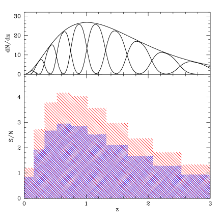
Figure 2: Top panel: the total expected LSST galaxy number distribution and its breakdown into ten photometric redshift bins. The distribution shown here is plotted using the parameters provided in the LSST white paper [17], and is slightly different from the one assumed in [14]. This difference does not lead to a noticeable change in any of the constraints on dark energy parameters. Bottom panel: the expected LSST/Planck cross-correlation signal-to-noise in each of the bins for the best fit LCDM model. The dark (red) shading corresponds to a half sky coverage by LSST, while the light (red) shading is for the full sky.

What we would like to address in the remainder of these proceedings is the utility of future measurements of the ISW effect. We will imagine correlating CMB data from Planck with photometric redshift galaxy catalogs from the proposed Large Synoptic Survey Telescope (LSST) [17]. The details of our assumptions for Planck and LSST can be found in [16]. We assume that LSST will cover half of the full sky and catalog around $50$ gal/arcmin² in ten photometric redshift bins spaced evenly between $z=0$ and $3$. The total galaxy number distribution and its breakdown into photometric bins are plotted as a function of redshift in the top panel of Fig. 2. Correlating CMB with galaxies in each of the photometric bins gives the ISW contribution at mean redshifts of different bins, allowing us to map the evolution of $\dot{\Phi}$ with time.

In order to put the discussion on a more quantitative footing we need to define some notation [18]. The CMB temperature is a function of the direction on the sky, $T(\hat{n})$. Its two-point auto-correlation function $C(|\hat{n}-\hat{n}^{\prime}|)=C(\theta)=\langle T(\hat{n})T(\hat{n}^{\prime})\rangle$ is usually decomposed into a Legendre series with coefficients $C_{\ell}$. It is common to evaluate the CMB angular spectrum, $\ell(\ell+1)C_{\ell}/2\pi$ vs $\ell$, which is the quantity plotted in Fig. 1. The distribution of galaxies in the $i$-th photometric bin is also a function of $\hat{n}$, $M^{(i)}(\hat{n})$. Here one can define Legendre coefficients $M^{(ij)}_{\ell}$ corresponding to the two-point correlation between galaxies in the $i$-th and the $j$-th bins. The cross-correlation between CMB and galaxies in one of the bins can be similarly represented in terms of the angular spectrum $X^{(i)}_{\ell}$ defined via

$$\langle T(\hat{n})M^{(i)}(\hat{n}^{\prime})\rangle\equiv X^{(i)}(\theta)=\sum_{\ell=0}^{\infty}{2\ell+1\over 4\pi}X^{(i)}_{\ell}P_{\ell}(\theta)$$ (2)

Figure 3: The angular spectrum of the correlation of the Planck CMB temperature with the $4$-th LSST bin in Fig. 2 for the best fit LCDM model. Shown are the statistical error bars based on a half (lager blue) and a full (smaller red) sky coverage by LSST.

The time-evolution of galaxy clustering is described by the so-called growth factor, $D(a)$, which in general relativity is scale-independent in the linear regime. The ISW contribution to the CMB anisotropy is sourced by the time-derivative of the gravitational potential, related to the growth factor via the Poisson equation: $\dot{\Phi}\propto d(D(a)/a)/d\eta$. The correlation between clustering and the CMB is essentially probing the quantity

$$P(\bar{z}_{i})=D(\bar{z}_{i})\left({d\over dz}[(1+z)D(z)]\right)_{z=\bar{z}_{i}}\,$$ (3)

where $\bar{z}_{i}$ is the mean redshift of a given bin. Having multiple bins, as in Fig. 2, would allow one to trace the evolution of $P(z)$ over a wide range of redshifts. Since, as shown in [3, 16, 19], it is an extremely sensitive probe of dark energy, even a marginal measurement of $P(z)$ would be of high value.

The statistical signal-to-noise (S/N) in $X^{(i)}_{\ell}$ is given by

$$\left({S\over N}\right)^{2}_{\ell}={f_{\rm sky}(2\ell+1)\over 4\pi}{(X^{(i)}_{\ell})^{2}\over C_{\ell}M_{\ell}^{(ii)}+(X^{(i)}_{\ell})^{2}}\ ,$$ (4)

and generally $C_{\ell}M_{\ell}^{(ii)}\gg(X^{(i)}_{\ell})^{2}$ because there is a large contribution to the $C_{\ell}$ coming from the last scattering epoch that does not correlated with the low-redshift universe. The S/N expected for the LCDM model in each of the LSST bins is shown in the bottom panel of Fig. 2.

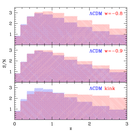
Figure 4: The expected signal-to-noise in correlation of the Planck CMB temperature with the LSST galaxies (Fig. 2) for three different dark energy models ($135^{\circ}$ red shading) compared to the best fit LCDM ($45^{\circ}$ blue shading). A half-sky LSST coverage is assumed. Shown are results the constant $w=-0.8$ and $w=-0.9$ models, and the kink model (Fig. 6). The Hubble parameter was adjusted to give nearly identical CMB spectra for all models being compared.

The distribution of the S/N can depend strongly on the particular dark energy model. In models with $w>-1$ dark energy starts to dominate earlier, leading to an earlier contribution to the ISW effect. The difference in the S/N for different models is shown in Fig. 4, where the Hubble parameter in each of the three case was adjusted to keep the peak structure of the CMB spectra nearly identical to the best fit LCDM. The difference is particularly pronounced for the so-called kink model, in which $w$ undergoes a sharp transition from a higher to lower value.

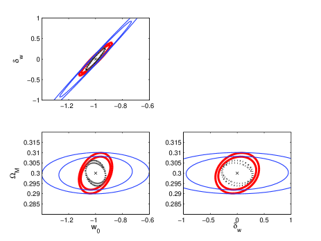
Figure 5: The $1\sigma$ projected Fisher contours for parameters of the model with $w$ given by eq. (5). Other parameters were marginalized over. The (blue) thin solid lines are for Planck’s CMB. Here, the larger contours are for temperature spectra alone, while the smaller ones include information from CMB polarization. The (red) think solid lines are constraints from CMB spectra combined with CMB correlation with LSST galaxies. The (black) dashed contours are for the supernovae from SNAP (using the assumptions of [21]) combined with Planck. The plot is taken from [16].

In [16] Fisher matrix analysis was used to forecast errors on evolving $w(z)$. Such forecasts, of course, depend on the choice of the model of $w(z)$ and the fiducial values of the parameters. Here we show results for two models. In Model I the parameterization is [20]

$$w(a)=w_{0}+(a-1)\delta_{w}$$ (5)

with fiducial values of the parameters chosen to represent the LCDM model: $w_{0}=-1$, $\delta_{w}=0$. The projected $1\sigma$ contours on these parameters and $\Omega_{M}$ are shown in Fig. 5. Spatial flatness and adiabatic initial conditions, favored by the WMAP data, were assumed. The usual cosmological parameters were also varied and marginalized over. It is clear that for this model the cross-correlations constraints on dark energy are informative, but somewhat weaker than those derived from the supernovae data.

To illustrate how the choice of the model can affect the forecasts, we also show results obtained in [16] for the so-called kink model. In the kink model, shown in Fig. 6, $w$ transitions from $-1$ at low redshifts to a higher value in the past. The supernovae would have a difficulty ”seeing” such a transition had it occurred at a sufficiently high redshift. The CMB/LSS correlation, on the other hand, can prove to be a useful tool in this case. We describe the kink in Fig. 6 using three parameters. Those are the width of the transition $\Delta_{z}$, the total change in the equation of state, $\Delta_{w}$, and the weighted average value $\langle w\rangle$ defined as

$$\langle w\rangle={\int da\Omega_{DE}(a)w(a)\over\int da\Omega_{DE}(a)}$$ (6)

This quantity controls the angular diameter distance to the last scattering [22]. Making $\langle w\rangle$ and explicit parameter has the advantage of being able to clearly separate models that fit the peak structure of the CMB angular spectrum from those that do not.

Figure 6: The $w(z)$ vs $z$ in the kink model with $\Delta_{z}=0.3$, $\Delta_{w}=-0.3$ and $\langle w\rangle=-0.9$ This model predicts CMB spectrum nearly identical to that with $w=const=\langle w\rangle$, shown with a dash line.

Fisher errors for the kink model parameters were calculated in [16] under the assumption of flat geometry and adiabatic initial conditions. In Fig. 7 we show the $1\sigma$ projected contours on $\Omega_{M}$, $\Delta_{w}$ and $\langle w\rangle$. The other parameters, including $\Delta_{z}$, are marginalized over. For this model the cross-correlation measurements can provide competitive constraints on dark energy evolution.

A more model-independent approach to forecasting constraints on $w(z)$ is provided by the principal component analysis introduced to dark energy studies in [23]. A study comparing the power of different types of dark energy experiments using the principal component approach was performed in [24]. It was shown that the CMB/LSS correlation can provide a constraint on one principal component of $w(z)$ which would be complementary to information provided by other probes. The CMB/LSS correlation, similar to the CMB auto-correlation, is sensitive to an averaged value of $w(z)$ with added weight at higher redshifts.

Constraining the dark energy equation of state is only one of several promising applications of the ISW effect. It can also be a potentially useful probe of dark energy clustering [25, 26, 13], and a unique tool for testing models that explain apparent cosmic acceleration through modifications of Einstein’s theory of gravity [2, 27].

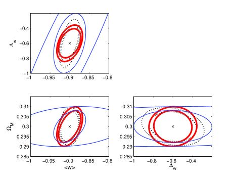
Figure 7: The $1\sigma$ projected Fisher contours for parameters of the kink model. $\Delta_{z}$ and other parameters were marginalized over. The meaning of the different lines is the same as in Fig. 5 – the contours corresponding to the cross-correlation of Planck and LSST, with added information from CMB spectra, are shown with (red) thick solid lines.

In summary, the ISW effect is not the most precise measurement we have in modern cosmology. However, with future surveys of large scale structure, such as LSST and the Square Kilometer Array (SKA) [28] covering large fractions of the sky and a wide range of redshifts, cross-correlation with CMB will likely become a standard tool for testing cosmological models that predict unconventional growth history at high to moderate redshifts. What allows the ISW effect to overcome the lack of accuracy is its extraordinary sensitivity to the details of the process of structure formation, whether it involves a scalar field dark energy, dark energy clustering or modifications of gravity. The ISW effect is free of some of the complicated physics involved in other probes of structure growth as it probes only linear scales, has a linear dependence on the galaxy bias, probes deep in redshift and is free of some of the degeneracies that hinder CMB studies on large scales. Given these strengths, and the fact that the utility of the ISW effect is a relatively under-researched subject, its most useful application may still be discovered in the future.

Acknowledgments

This talk was based on collaborations with R. Crittenden, P-S. Corasaniti, J. Garriga, R. Nichol, C. Stephan-Otto and T. Vachaspati. I would like to thank A. Cooray, M. Kaplinghat and all others involved in organizing the Fundamental Physics with CMB workshop at Irvine for putting togheter this timely and enjoyable meeting.

References

- [1] R. K. Sachs and A. M. Wolfe, Ap. J. 147, 73 (1967).
- [2] P. Zhang, Phys.Rev. D73 (2006) 123504, astro-ph/0511218.
- [3] A. Cooray, D. Huterer, and D. Baumann, Phys.Rev. D69 (2004) 027301, astro-ph/0304268.
- [4] M. Kamionkowski and A. Loeb, Phys.Rev. D56 (1997) 4511-4513, astro-ph/9703118.
- [5] J. Portsmouth, Phys.Rev. D70 (2004) 063504, astro-ph/0402173.
- [6] N. Seto and E. Pierpaoli, Phys.Rev.Lett.95 (2 005) 101302, astro-ph/0502564.
- [7] E. F. Bunn, Phys.Rev. D73, 123517 (2006), astro-ph/0603271.
- [8] M. Kesden, M. Kamionkowski, A. Cooray, Phys.Rev.Lett. 91 (2003) 221302, astro-ph/0306597.
- [9] R. Crittenden and N. Turok, Phys.Rev.Lett.76 (1996) 575, astro-ph/9510072.
- [10] S. Boughn and R. Crittenden, Nature 427 (2004) 45-47, astro-ph/0305001; N. R. Nolta et al, Astrophys.J. 608 (2004) 10-15, astro-ph/0305097; P. Fosalba and E. Gaztanaga, MNRAS 350 (2004) L37-L41, astro-ph/0305468; P. Fosalba et al, Astrophys.J. 597 (2003) L89-92, astro-ph/0307249; R. Scranton et al, astro-ph/0307335; N. Afshordi et al, Phys.Rev. D69 (2004) 083524, astro-ph/0308260; P. Vielva et al, MNRAS 365 (2006) 891-901, astro-ph/0408252; N. Padmanabhan et al, Phys.Rev. D72 (2005) 043525, astro-ph/0410360; McEwen et al, astro-ph/0602398; A. Cabre et al, astro-ph/0603690;
- [11] Ryan Scranton, talk given at the workshop on external correlations of CMB, Fermilab, May 25-27, 2006.
- [12] E. Gaztanaga, M. Manera, T. Multamaki, MNRAS 365 (2006) 171-177, astro-ph/0407022.
- [13] P-S. Corasaniti, T. Giannantonio, A. Melchiorri, Phys.Rev. D71 (2005) 123521, astro-ph/0504115.
- [14] A. Cooray, P-S. Corasaniti, T. Giannantonio, A. Melchiorri, Phys.Rev. D72 (2005) 023514, astro-ph/0504290.
- [15] D. Spergel et al (WMAP collaboration), astro-ph/0603449.
- [16] L.Pogosian, P. S. Corasaniti, C. Stephan-Otto, R. Crittenden, and R. Nichol, Phys.Rev. D72 (2005) 103519, astro-ph/0506396.
- [17] http://www.lsst.org
- [18] J. Garriga, L. Pogosian, and T. Vachaspati, Phys.Rev. D69 (2004) 063511, astro-ph/0311412.
- [19] L. Pogosian, JCAP 0504 (2005) 015, astro-ph/0409059.
- [20] M. Chevallier, D. Polarski, Int.J.Mod.Phys. D10 (2001) 213-224, gr-qc/0009008; E. V. Linder, Phys.Rev.Lett. 90 (2003) 091301, astro-ph/0208512.
- [21] A. G. Kim, E. V. Linder, R. Miquel, N. Mostek, MNRAS 347 (2004) 909-920, astro-ph/0304509.
- [22] G. Huey et al, Phys.Rev. D59 (1999) 063005, astro-ph/9804285; T. D. Saini, T. Padmanabhan, S. Bridle, MNRAS 343 (2003) 533, astro-ph/0301536.
- [23] D. Huterer and G. Starkman, Phys.Rev.Lett. 90 (2003) 031301, astro-ph/0207517.
- [24] R. Crittenden and L. Pogosian, astro-ph/0510293.
- [25] R. Bean and O. Dore, Phys.Rev. D69 (2004) 083503, astro-ph/0307100
- [26] W. Hu and R. Scranton, Phys.Rev. D70 (2004) 123002, astro-ph/0408456.
- [27] Y-S. Song, I. Sawicki, W. Hu, astro-ph/0606286
- [28] http://www.skatelescope.org/