Description of Stellar Acoustic Modes
Using the Local Wave Concept

Abstract

An understanding of stellar acoustic oscillations is attempted, using the local wave concept in semi-analytical calculations. The local homogeneity approximation allows to obtain simplified equations that can nevertheless describe the wave behavior down to the central region, as the gravitational potential perturbation is not neglected. Acoustic modes are calculated as classical standing waves in a cavity, by determining the cavity limits and the wave phases at these limits. The internal boundary condition is determined by a fitting with an Airy function. The external boundary condition is defined as the limit where the spatial variation of the background is important compared to the wavelength. This overall procedure is in accordance with the JWKB approximation. When comparing the results with numerical calculations, some drawbacks of the isothermal atmosphere approximation are revealed. When comparing with seismic observations of the Sun, possible improvements at the surface of solar models are suggested. The present semi-analytical method can potentially predict eigenfrequencies at the precision of $\pm$3 $\mu$Hz in the range 800-5600 $\mu$Hz, for the degrees $l=0-10$. A numerical calculation using the same type of external boundary conditions could reach a global agreement with observations better than 1 $\mu$Hz. This approach could contribute to better determine the absolute values of eigenfrequencies for asteroseismology.

1 Introduction

Asteroseismology describes mainly the propagation of matter waves and their eigenmodes in stars (or planets) that are considered as cavities. By an inverse procedure one can then deduce the physical properties of the layers crossed by the waves. It is a very effective tool, and often the unique one to study the internal structure of stars. Since several decades, many intensive works were undertaken, especially for the Sun, to calculate precisely the oscillation modes and to understand the physical mechanisms involved. Different reviews are dedicated to this subject (Cox, 1980; Unno et al., 1989; Christensen-Dalsgaard & Berthomieu, 1991; Turck-Chièze et al., 1993; Christensen-Dalsgaard, 1998).

Semi-analytical approaches have been developed, essentially based on various asymptotic approximations. Lamb (1909, 1932), Cowling (1941), Tassoul (1980), Leibacher & Stein (1981), Duvall (1982), and Deubner & Gough (1984), have explored the first-order asymptotic approximation, and have helped to interpret the high-order modes measured for the Sun. Then with the availability of low-order modes, Vorontsov (1991), Lopes & Turck-Chièze (1994),Roxburgh & Vorontsov (2000), have taken into account the effect of gravity in second-order theories, allowing to better describe the propagation in central regions of stars. On another hand, numerical calculations are required to reach the high precision in frequency determination, needed for inversion of stellar internal layer physics. Several high accuracy oscillation codes already exist, offering the computation of eigenfrequencies and eigenfunctions (Christensen-Dalsgaard, 1982; Unno et al., 1989). They have been widely used to interpret the large amount of solar modes observed from Earth or space.

Just at the beginning of the spatial-asteroseismology era, it is worth assessing the progress of these theoretical efforts in the prediction of observations. It is interesting to note that the agreement between numerical results and observations is remarkable in the range 1000 - 2400 $\mu$Hz where $\nu_{num}-\nu_{obs}$ is contained in $\pm$1 $\mu$Hz. At larger frequencies however, the disagreement increases gradually, up to 20 $\mu$Hz at 5000 $\mu$Hz. Semi-analytical results agree well with numerical ones only in that high-frequency range, while their dispersion at lower frequencies stays important even when they have been reduced by the second order approximation. Moreover, the acoustic cut-off frequency is theoretically predicted around 5000 $\mu$Hz, while from observations it is rather around 5600 $\mu$Hz (Fossat et al., 1992; García et al., 1998). Those difficulties can be overcome in the case of the Sun thanks to the great number of eigenmodes accessible by observations. But such difference could be more problematic in asteroseismology as only low-degree modes ($l\leq 3$) are available and the stellar radius and mass are less known.

The discrepancy between calculation and observation is generally attributed to an incorrect description of the outer layers of the current solar models at the surface. Several studies have tried to introduce a more relevant model of convection via the introduction of a turbulent pressure (Kosovichev, 1995). That reduces the discrepancy at high frequencies, but the excellent agreement at low frequencies is also deteriorated (Rosenthal et al., 1995, 1999). The role of the chromosphere was also invoked, but no real improvement is yet obtained (Wright & Thompson, 1992; Vanlommel & Goossens, 1999; Dzhalilov et al., 2000).

With the regular progress of observational instruments, these remaining problems become more crucial: the theory-observation discrepancies at high frequencies and the inaccuracy of semi-analytical methods at low frequencies are up to 100 times larger than observational errors. So, we suggest to search the reasons not only in the solar model at the surface, but also in the eigenmode calculation itself, especially about the wave description in the solar interior and the boundary conditions at the surface. Concepts closer to classical wave physics remain to be further explored. It can be considered as a continuation of the works of Leibacher & Stein (1981) and Duvall (1982). Some first acoustic-frequency calculations was attempted in Nghiem (2000), and the effect of gravitational potential was taken into account in Nghiem (2003a). In this paper, we aim to further formalize the concepts, by putting a special accent on the internal and external boundary conditions. This work is organized as follows. In §2, a new p-mode calculation is developed. Its approximations and its boundary conditions are proved to be in accordance with the JWKB method. In §3, the obtained results are first compared to present numerical calculations, and some drawbacks of the isothermal atmosphere approximation are pointed out. Then in §4 comparisons with observations suggest a way to improve solar surface descriptions, and at the same time to evaluate the potential of the proposed method. Concluding remarks are presented in §5.

In this paper, the solar model used is the seismic model (Turck-Chièze et al., 2001; Couvidat et al., 2003), computed with the CESAM code (Morel, 1997). The numerical results for solar oscillations are obtained with the ADIPLS code (Christensen-Dalsgaard, 1997). Acoustic mode observations of the Sun come from the SoHO spacecraft (MDI data from Rhodes et al. (1997); GOLF data from Bertello et al. (2000), and from García et al. (2001).The graphic representation for modes of degrees $l=0$ to 10 follows the symbols indicated in Figure 1.

Figure 1: Symbols used for the graphic representation of the $l=0$ to 10 modes in all this paper.

2 The Present Approach

The present study starts from the standpoint that observed solar modes, due to their regularity and their precision, are related to waves in its most classical sense, excluding shock waves, wave buckets, etc. Basically eigenfrequencies are the signature of waves trapped in a cavity. A wave is the propagation of an oscillation. An oscillation is a continuous exchange between kinetic and potential energy around an equilibrium state. Here the notion of equilibrium state is the central one. Where this latter ends, there is no possible oscillation, thus no more propagation, the wave becomes evanescent. At this point, the wave is reflected. That determines the turning point, i.e. the cavity limit.

Inside a huge gazeous sphere maintained by gravity like a star, two kinds of equilibrium can be considered: the equilibrium between stratums of different pressure, and the pressure equilibrium inside each stratum, that is the local homogeneity. Every pressure perturbation generates two oscillations: a gravity one around an equilibrium stratum, and an acoustic one around a point of local equilibrium. The two induced waves do not interact between them, unless their frequencies are close to each other. For the Sun, excepted around 500 $\mu$Hz where coupling has to be considered, acoustic and gravity waves can be studied separately. The present approach is also applicable for all stars where acoustic and gravity frequencies are well separated.

Let us now concentrate only on pure acoustic waves. By definition, such a wave can only propagate in a locally homogeneous environment, or more precisely homogeneous as regard to its wavelength. If the pressure scale height can be seen as representative of the homogeneity, the propagation condition can be expressed as

$$\lambda=\frac{2\pi}{k}<aH_{p(\mathbf{k})}$$ (1)

where $\lambda$ is the wavelength, $k$ the wavenumber, $H_{p(\mathbf{k})}$ the pressure scale height projected on the propagation direction $\mathbf{k}$, and $a$ is a constant to be determined. To be exhaustive, this coefficient could be considered as the first one of a Taylor expansion in $\lambda$, $H_{p}$, $H_{\rho}$, or similar parameters. These coefficients should be determined once, by experiments on Earth, or spatial experiments, or theoretical studies, but they are not specific to a star. When a condition of the type of equation (1) is no longer satisfied, the wave can no longer propagate and is reflected.

The reflection conditions are different, following the current pressure variation. If that happens where the pressure is increasing, for the wave, everything is like it encounters a wall, the reflection gets the properties of the ‘pressure wall’ type. On the opposite case, that are the properties of the ‘pressure vacuum’ type. For this latter, in the absence of any other force, the force balance at the boundary requires that the perturbed pressure at the discontinuity is

$$p^{\prime}=0.$$ (2)

One must have a pressure node, corresponding to a displacement antinode, because, as seen below, there is a phase lag of $\pi$/2 between them. We will see that it is the case at the upper atmosphere limit: the last layer freely vibrates under the action of acoustic waves. The situation is exactly the same at the free end of a spring laying horizontally on a frictionless surface on Earth. Now, in the presence of the gravity force, the force balance requires that

$$p^{\prime}+\rho_{0}\int\!\!g^{\prime}\!dr=0$$ (3)

where $g^{\prime}$ is the perturbed gravity, and $\rho_{0}$ is the equilibrium density that can be brought out the integral thanks to the local homogeneity approximation. Note that the sign used in this context is opposite to that of the continuity equation. As seen later, this will be the situation for the radial mode at the internal boundary. This looks like vibrations at the free end of a spring vertically hung in the Earth gravity field.

From this viewpoint, the reflexion occurs at a given radius, and the continuity condition must be regarded at the two sides of this fixed limit, thus the perturbed pressure considered should be eulerian. This is different from the perspective where the limit is not fixed in space but follows the displacement generated by the perturbation, where the lagrangian perturbed pressure is considered.

The wave propagation and reflection are so far completely defined in their principles. We are in the approximation context of local homogeneity, or pure acoustic wave, or of local wave, i.e. the wave is only defined locally. It is important to stress that in this approximation, the environment is not homogeneous, but slowly variable. This choice is only guided by the aim of describing what is called a ‘local-acoustic’ wave. The precision reached with this approximation is not known a priori, so it will be estimated on the view of its expressions and its numerical results, compared to other methods.

2.1 Wave Propagation

After a perturbation, the wave propagation is fully described by the four eulerian functions $\xi$, $p^{\prime}$, $\rho^{\prime}$, $\Phi^{\prime}$, which are respectively the displacement, along with the perturbations of pressure, density and gravitational potential. In the hypotheses of adiabacity, sphericity and linearity, and when the time, angular, and radial parts have been separated, these unknown functions are governed by the following differential equations where only remains the radial part (see e.g. Christensen-Dalsgaard (1998), p.54):

$$\frac{d\xi_{r}}{dr} = \left(-\frac{2}{r}+\frac{1}{\Gamma_{1}H_{p}}\right)\xi_{r}+\left(\frac{l(l+1)}{r^{2}}-\frac{\omega^{2}}{c_{0}^{2}}\right)\frac{p^{\prime}}{\rho_{0}\omega^{2}}$$ (4)

$$-\frac{l(l+1)}{\omega^{2}r^{2}}\Phi^{\prime}$$

$$\frac{dp^{\prime}}{dr} = \rho_{0}(\omega^{2}-N^{2})\xi_{r}-\frac{1}{\Gamma_{1}H_{p}}p^{\prime}+\rho_{0}\frac{d\Phi^{\prime}}{dr}$$ (5)

$$\rho^{\prime} = \frac{p^{\prime}}{c_{0}^{2}}+\frac{\rho_{0}}{g_{0}}N^{2}\xi_{r}$$ (6)

$$\frac{d^{2}\Phi^{\prime}}{dr^{2}} = -\frac{2}{r}\frac{d\Phi^{\prime}}{dr}-4\pi G\rho^{\prime}+\frac{l(l+1)}{r^{2}}\Phi^{\prime}$$ (7)

with r the distance to the stellar center, and $l$ the mode degree. The other symbols stand for medium equilibrium quantities: $p_{0}$, $\rho_{0}$, $c_{0}$, $g_{0}$ are the pressure, the density, the sound speed, and the gravity; $H_{p}$ is the pressure scale height, $N$ the buoyancy frequency, and $\Gamma_{1}$ the adiabatic exponent. That is in fact a system of 3 differential equations of fourth order. Equation (6) in $\rho^{\prime}$ is added only for the sake of exhaustiveness.

That system of differential equations can only be solved numerically. An analytical solution needs further approximations. Due to that, results obtained by numerical codes are more precise and realistic than those of analytical methods. Nevertheless, the final result crucially depends on boundary conditions that are not contained in those equations. The choice of boundary conditions comes from physical considerations, and analytical calculations can be helpful for that, especially when their results are precise enough to be not too far from numerical ones, or in other words, and that is an evidence, when the approximations used are not too crude.

In order to find an analytical solution, we propose to use the above suggested approximation of local homogeneity (but not of homogeneity), where the derivatives of the equilibrium quantities are only negligible when compared to equilibrium quantities themselves. Only the relative derivatives, namely $1/H_{p}$, $1/H_{\rho}$, and thus $N^{2}$, can be neglected. This also mathematically justify a validity condition of the type of equation (1). In that context, equations (4-7) become:

$$\frac{d\xi_{r}}{dr} = -\frac{2}{r}\xi_{r}+\left[\frac{l(l+1)}{r^{2}}-\frac{\omega^{2}}{c_{0}^{2}}\right]\frac{p^{\prime}}{\rho_{0}\omega^{2}}$$ (8)

$$-\frac{l(l+1)}{\omega^{2}r^{2}}\Phi^{\prime}$$

$$\frac{dp^{\prime}}{dr} = \rho_{0}\omega^{2}\xi_{r}+\rho_{0}\frac{d\Phi^{\prime}}{dr}$$ (9)

$$\rho^{\prime} = \frac{p^{\prime}}{c_{0}^{2}}$$ (10)

$$\frac{d^{2}\Phi^{\prime}}{dr^{2}} = -\frac{2}{r}\frac{d\Phi^{\prime}}{dr}-4\pi G\rho^{\prime}+\frac{l(l+1)}{r^{2}}\Phi^{\prime}.$$ (11)

Using equations (8-11), the derivative of equation (9) gives

$$\frac{d^{2}p^{\prime}}{dr^{2}}+\frac{2}{r}\frac{dp^{\prime}}{dr}+\left[\frac{\omega^{2}+4\pi G\rho_{0}}{c_{0}^{2}}-\frac{l(l+1)}{r^{2}}\right]p^{\prime}=0.$$ (12)

When searching for a spherical solution $p^{\prime}=P^{\prime}/r$, $P^{\prime}$ must verify

$$\frac{d^{2}P^{\prime}}{dr^{2}}+\left[\frac{\omega^{2}+4\pi G\rho_{0}}{c_{0}^{2}}-\frac{l(l+1)}{r^{2}}\right]P^{\prime}=0.$$ (13)

This typical wave equation with slowly variable coefficients has a well known solution in the JWKB approach (see appendix A), so that

$$p^{\prime}(r)=\frac{A}{r\sqrt{k_{r}}}\cos\left(-\int_{r_{0}}^{r}\!\!k_{r}dr+\psi\right).$$ (14)

By searching a solution of the same type for $\Phi^{\prime}$, equation (11) gives the particular solution

$$\Phi^{\prime}(r)=\frac{4\pi G}{c_{0}^{2}k^{2}}\frac{A}{r\sqrt{k_{r}}}\cos\left(-\int_{r_{0}}^{r}\!\!k_{r}dr+\psi\right)$$ (15)

and finally equation (9) gives

$$\xi_{r}(r)=\frac{A\sqrt{k_{r}}}{r\rho_{0}c_{0}^{2}k^{2}}\sin\left(-\int_{r_{0}}^{r}\!\!k_{r}dr+\psi\right).$$ (16)

Thus $\xi_{r}$ differs by $\pi/2$ in phase with $p^{\prime}$, $\rho^{\prime}$ and $\Phi^{\prime}$. Remark also that $r_{0}$ and $r$ should be in a domain where $k_{r}\geq 0$. Otherwise exponential solutions should be considered. To be exhaustive, a general solution has to be added to the particular solution $\Phi^{\prime}$, but it will play a role only for radial modes very near the center, so we will invoke it only in section 2.7.

Equations (14-16) are the expressions of a spherical wave that is well defined only locally. The amplitude $A$ and the phase $\psi$ are not constant but almost constant. At a given radius $r$, the radial wavenumber $k_{r}$ is given by

$$k_{r}^{2}=\frac{\omega^{2}+4\pi G\rho_{0}}{c_{0}^{2}}-\frac{l(l+1)}{r^{2}}$$ (17)

and, for a spherical wave, its horizontal component is

$$k_{h}^{2}=\frac{l(l+1)}{r^{2}}.$$ (18)

Thus the wave number is

$$k^{2}=\frac{\omega^{2}+4\pi G\rho_{0}}{c_{0}^{2}}.$$ (19)

The amplitude of the radial displacement is further evaluated in appendix B. The sound speed, or the phase velocity of the sound wave is (in a propagative medium where $k^{2}>0$)

$$v_{\varphi}=\frac{\omega}{k}=\frac{c_{0}}{\sqrt{1+4\pi G\rho_{0}/\omega^{2}}}$$ (20)

which is equal to $c_{0}$ only when $4\pi G\rho_{0}/\omega^{2}$ is negligible compared to 1.

This propagative wave solution is surprisingly simple. Discussions about its relevance are needed, as well in the interior than at the surface of the star.

2.2 Relevance in the Stellar Interior

In the stellar interior, a wave solution given by equations (14-16) are all the more simple as the gravitational perturbation is already taken into account. There is no need to develop to higher orders in $\Phi^{\prime}$. The latter is considered at the same rank than the other perturbations $\xi$, $p^{\prime}$, and $\rho^{\prime}$, like it should be naturally. The final results obtained should be more precise and more realistic. Indeed, as only the relative gradients of equilibrium quantities are neglected, and not the gradients themselves, the gravity that is linked to the pressure gradient is not neglected. Physically, acoustic waves have enough short wavelengths not to see the gravitational stratification at large scale, but they will progressively pass through a non constant, hydrostatic structure governed by gravity. The non-negligible gravitational potential and its perturbation are seen by the term $4\pi g\rho^{\prime}$ in equation (11).

The consequence is that the obtained accuracy will be the same for all ranges of $l$ or $\omega$ (except for frequencies near gravity frequencies), contrary to restrictions of large $l$ or $\omega$ imposed by more drastic asymptotic approximations.

Another advantage is the autocoherence concerning the spherical eigenvalue $l(l+1)$ which will be maintained the same all along the present study. There is no need to replace it by $(l+0.5)^{2}$, a trick sometimes employed at low-$l$ (!), whose the artificial character is clearly pointed out in Langer (1937). It is also easy now to bring an answer to the controversial question about the fact that the radial mode ($l=0$) reaches or not the center: due to its spherical nature, described by the term in $A/r$ in equation (14), the wave can never touch the center, whatever the value of $l$. The non-radial waves reach their internal turning points where $k_{r}=0$, while the case of radial waves are examined in details in section 2.7 below.

2.3 Relevance at the stellar Surface

At the surface, the term $4\pi G\rho_{0}$ can be neglected, equation (17) becomes

$$k_{r}^{2}=\frac{\omega^{2}}{c_{0}^{2}}-\frac{l(l+1)}{r^{2}}$$ (21)

and generally, for not too large $l$,

$$k_{r}=\frac{\omega}{c}$$ (22)

which is particularly simple. The important issue is that $k_{r}$ continuously increases toward the surface. Yet it was established by current asymptotic approximations that the expression of $k_{r}$ goes to zero near the surface, and that location could be considered as the external turning point. Does it mean that equation (21) is obtained in a too approximated context, and some terms could have been missed? It is actually possible to derive a less approximated propagation equation than equation (13), in the following way.

At the surface, and for not too large $l$, it is legitimate to remove the terms $2/r$, $l(l+1)/r^{2}$, and the terms in $\Phi^{\prime}$ from equations (4-5), which become

$$\frac{d\xi_{r}}{dr} = \frac{1}{\Gamma_{1}H_{p}}\xi_{r}-\frac{p^{\prime}}{\rho_{0}c_{0}^{2}}$$ (23)

$$\frac{dp^{\prime}}{dr} = \rho_{0}(\omega^{2}-N^{2})\xi_{r}-\frac{1}{\Gamma_{1}H_{p}}p^{\prime}.$$ (24)

Providing that

$$\frac{1}{c_{0}^{2}}\frac{dc_{0}^{2}}{dr}=\frac{1}{\Gamma_{1}p_{0}}\frac{d(\Gamma_{1}p_{0})}{dr}+\frac{1}{H_{\rho}},$$ (25)

$$\frac{N^{2}}{c_{0}^{2}}=-\frac{1}{(\Gamma_{1}Hp)^{2}}+\frac{1}{\Gamma_{1}H_{p}H_{\rho}}$$ (26)

and using equations (23-24) in the derivation of equation (23), one obtains:

$$\!\!\!\!\!\!\!\!\frac{d^{2}\xi_{r}}{dr^{2}}\!\!\!\! + \!\!\!\!\frac{1}{\Gamma_{1}p_{0}}\frac{d(\Gamma_{1}p_{0})}{dr}\frac{d\xi_{r}}{dr}$$ (27)

$$+ \!\!\!\!\left(\frac{\omega^{2}}{c_{0}^{2}}-\frac{1}{\Gamma_{1}H_{p}H_{\rho}}+\frac{1}{\Gamma_{1}p_{0}}\frac{d^{2}p_{0}}{dr^{2}}\right)\xi_{r}=0$$

To avoid the term in $d\xi_{r}/dr$, introduce $K$ as:

$$\xi_{r}=K\exp\left(-\frac{1}{2}\int\!\!\frac{1}{\Gamma_{1}p_{0}}\frac{d(\Gamma_{1}p_{0})}{dr}\!dr\right)$$ (28)

to obtain the propagation equation:

$$\!\!\!\!\!\!\!\!\!\!\!\!\frac{d^{2}K}{dr^{2}}+\Bigg{\{}\frac{\omega^{2}}{c_{0}^{2}}-\frac{1}{\Gamma_{1}H_{p}H_{\rho}}+\frac{1}{\Gamma_{1}p_{0}}\frac{d^{2}p_{0}}{dr^{2}}$$ (29)

$$\!\!\!\!\!\!\!\!\!\!\!\!-\frac{1}{4}\left[\frac{1}{\Gamma_{1}p_{0}}\frac{d(\Gamma_{1}p_{0})}{dr}\right]^{2}-\frac{1}{2}\frac{d}{dr}\left[\frac{1}{\Gamma_{1}p_{0}}\frac{d(\Gamma_{1}p_{0})}{dr}\right]\Bigg{\}}K=0.$$

Equation (29) is a generalization of what is derived in current asymptotic approximations. Indeed, when $g$ is constant, the two terms after $\omega^{2}/c_{0}^{2}$ cancel each other out, and if further more $\Gamma_{1}$ is constant, it looks more familiar (Deubner & Gough, 1984):

$$\frac{d^{2}K}{dr^{2}}+\left[\frac{\omega^{2}}{c_{0}^{2}}-\frac{1}{4H_{p}^{2}}\left(1+2\frac{dH_{p}}{dr}\right)\right]K=0.$$ (30)

At the surface, these last equations are indisputably less approximated than those obtained in the local homogeneity approximation. The deduced $k_{r}$ goes to zero near the surface. But for all that, are those last expressions more relevant? Can them be used to determine the external turning points?

To answer, a detour by the JWKB approach is necessary. Following appendix A, equations (29, 30) admit a wave-like solution only when the conditions of equation (A7) are verified, i.e. when properties of the medium vary slowly. The JWKB approximation also predicts that in these conditions, there is no wave reflection, or at least the reflections are negligible. In the opposite case, there is no wave-like solution and reflections will occur.

An important consequence is that, generally, in order to be able to apply JWKB, the expression of $k_{r}(r)$ can only contain medium variables at the same derivation order. For example, if the equilibrium pressure $p_{0}$ appears in $k_{r}(r)$, then the derivatives $dp_{0}/dr,d^{2}p_{0}/dr^{2}$ must be negligible, if not the conditions of equation (A7) cannot be verified (except for very specific cases). If it contains $dp_{0}/dr$, then it should contain neither $p_{0}$ nor $d^{2}p_{0}/dr^{2},d^{3}p_{0}/dr^{3}$.

Another consequence is that when the JWKB approximation is applicable, and only in this case, the sign of $k_{r}^{2}$ indicates the propagation or evanescent character. It is also clear that when $k_{r}(r)=0$, the conditions of equation (A7) are of course violated, and there is reflection. But we should not forget that reflection immediately occurs whenever those conditions are no more valid, even when $k_{r}(r)$ is very far from zero. And we should keep in mind that those reflection conditions are not contained in the expression of $k_{r}$ alone.

It appears therefore that the $k_{r}$ deduced from equations (29) or (30) contains $p_{0},\rho_{0}$ as well as their derivatives, thus is generally rapidly variable, thus the JWKB approach cannot be applied, and its zeros have no special physical sense. It just means that when the relative derivatives of equilibrium quantities cannot be neglected, we are in the evanescent part, outside the resonant cavity. This is coherent with the local-homogeneity analysis. (In fact, equation (30) indicates that the JWKB method can nevertheless be applied in the very special case where both $c_{0}$ and $H_{p}$ are slowly variable, so that $H_{p}^{-2}dH_{p}/dr$ can be neglected. It is the case for an isothermal atmosphere which will be discussed further in section 3.3).

On the contrary, in the context of local homogeneity, i.e. slowly variable medium, the $k_{r}$ obtained in equation (17) automatically satisfies the JWKB application conditions. In the present case of spherical modes, the internal cavity limits are generally situated towards the center where the medium is really slowly variable, and the turning points will be determined by $k_{r}(r)=0$, or very close to that. Concerning the external limit, the cause of rapidly variable medium should rather be invoked. In other words, an acoustic wave turns back in the interior because of its own spherical nature, and at the surface because of an abrupt medium change. This internal/external dissymmetry can be seen on the wave trajectories (Fig. 2).

From that long but necessary discussion, it can be concluded that conceptually, the local homogeneity approximation and its cavity limit criteria are nothing but a physical translation of the JWKB mathematical expression.

Figure 2: Wave trajectories for the mode $l=5,n=5$. Internal and external turning points are indicated by the arrows, which show their different behaviours.

2.4 Wave Trapping

When the acoustic wave is reflected at the external and internal limits of a star, we are in the presence of standing waves inside a cavity, where only determined frequencies will be favoured. The sum of forward and backward waves forms standing waves with nodes and antinodes separated by $\pi$ in phase

$$y(r) = \frac{A}{r}\cos\left(\omega t-\int_{r_{0}}^{r}\!\!k_{r}dr+\psi\right)$$

$$+ \frac{A}{r}\cos\left(\omega t-\int_{r}^{r_{0}}\!\!k_{r}dr+\psi^{\prime}\right)$$

$$=\frac{2A}{r}\cos(\omega t+\frac{\psi+\psi^{\prime}}{2})\cos\left(-\int_{r_{0}}^{r}\!\!k_{r}dr+\frac{\psi-\psi^{\prime}}{2}\right)$$ (31)

where $y$ stands for $\xi_{r}$, or $p^{\prime}$, or $\rho^{\prime}$ or $\Phi^{\prime}$ . Following Figure 3, it is clear that the phase advance between the turning points $r_{1}$ and $r_{2}$ should verify

$$\int_{r_{1}}^{r_{2}}\!\!k_{r}dr=(n+\alpha)\pi$$ (32)

where $n$ is the number of nodes along r, called the mode order, and $\alpha$ is a parameter to adjust following the phase conditions at $r_{1}$ and $r_{2}$. For example, if there are two antinodes at the two limits, $\alpha=0$, if there are one node and one antinode, $\alpha=-0.5$. If there are two nodes, $\alpha=-1$. The convention adopted here is to count every node of the displacement $\xi_{r}$.

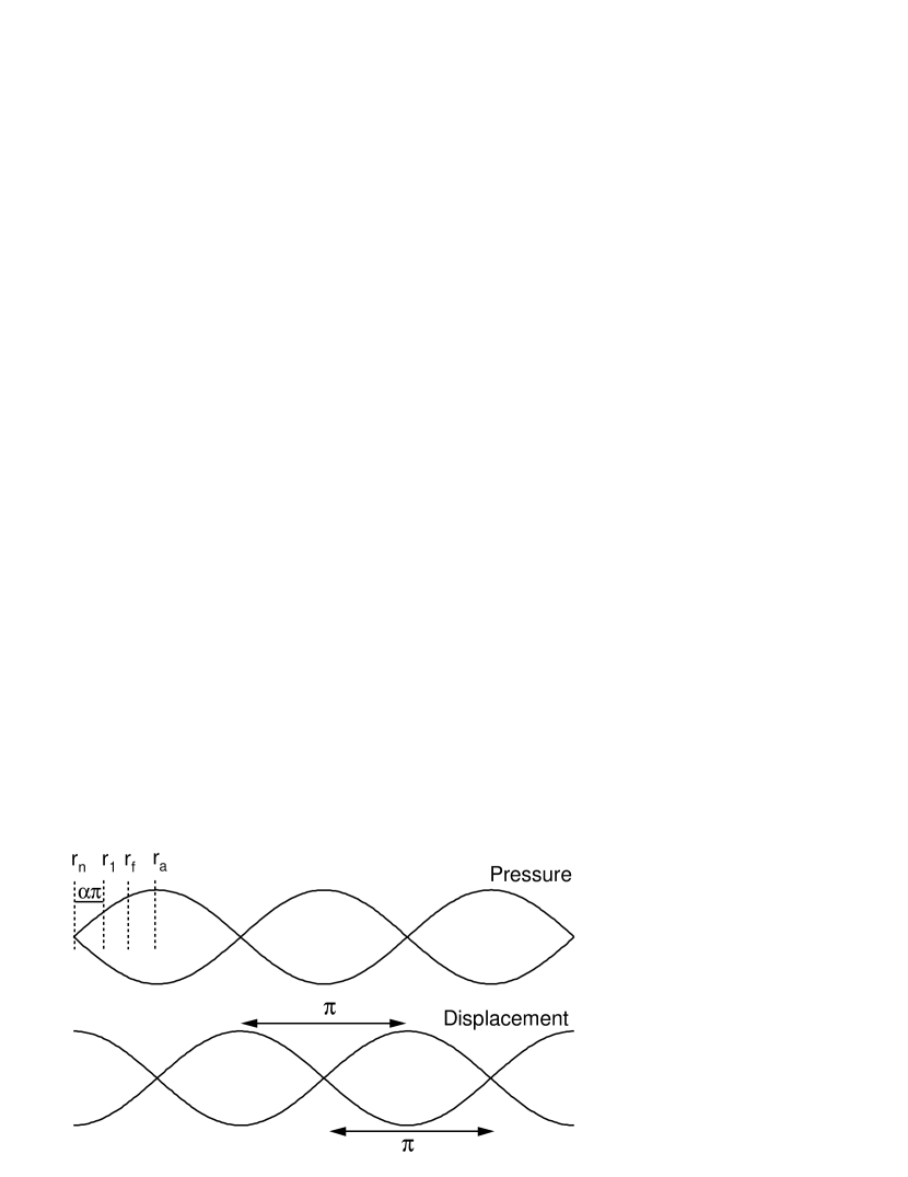
Figure 3: Acoustic standing wave with nodes and antinodes separated by $\pi$ in phase. Pressure and displacement differs by $\pi/2$ in phase. For the pressure, the locations of the internal node, turning point, fitting point, and antinode are marked by $r_{n}$, $r_{1}$, $r_{f}$, and $r_{a}$

.

The relation (32) is largely used in different approaches for interpreting solar acoustic eigenfrequencies (Duvall, 1982). Even so, attention must be paid that $r_{2}$ is sometimes assimilated to R, the star radius, while it is not the case here. This apparently small subtility is in fact fundamental. Indeed, assuming $r_{2}\equiv R$ is a crude approximation leading to frequency errors of tens of $\mu$Hz. Any attempt to compensate it, amounts to make a variable change while integrating (32), therefore to work with a wavenumber $k_{r}$ that is not the real one. So $\alpha$ is not the same than that employed here. Moreover, the phase conditions at external and internal turning points are completely mixed. The overall consequence is that one is not working in the real world, but in a kind of phase space.

Here, by working with $r_{2}$ and not R, the eigenmode determination becomes similar to what is done for an acoustic cavity on Earth, just like for any musical instrument. The eigenfunctions projected on the radial direction are given by the standing wave expression (eq. 31), and the eigenfrequencies are determined by the Duvall expression (32). Thus, to obtain the full solution it only remains to determine the internal and external turning points together with the phase conditions at these points, i.e. namely $r_{1}$, $r_{2}$ and $\alpha$.

2.5 External Turning Point

Let us begin to look at the external reflection conditions because they are the simplest ones, for the phase as well as for the location.

Following what has been discussed in section 2, at the surface, the acoustic wave is reflected when a ‘pressure vacuum’ is encountered. For the wave, everything looks like the end of the matter. Like any matter wave encountering a ‘matter vacuum’, there is an antinode at this point for the displacement (think e.g. about longitudinal standing waves along a spring with a free end). That determines the phase.

For the location of reflection, we must look at the projection of $H_{p}$ onto the propagation direction. Neglecting the surface curvature (see Figure 4), the propagation condition, equation (1), becomes

$$\frac{k^{2}}{k_{r}}=\frac{1}{k_{r}}\frac{\omega^{2}}{c_{0}^{2}}>\frac{2\pi}{a_{v}H_{p}}$$ (33)

knowing that the phase speed (eq. 20) at the surface is $c_{0}$. The constant $a_{v}$, v standing for vacuum, remains to be determined. This task concerns typically the boundary conditions that cannot be already included in the initial differential equations. Something else than the physics of wave propagation should be considered. In order to avoid theoretical results which are not totally reliable at the surface, we can choose the experimental Sun’s cut-off frequency combined with the semi-empirical atmosphere of Vernazza et al. (1981). According to Fossat et al. (1992) and García et al. (1998), the observed Sun’s cut-off frequency is

$$5600\pm 150\mu Hz.$$ (34)

In this frequency range and at the surface, equation (33) can be simplified to

$$\frac{\omega}{c_{0}}>\frac{2\pi}{a_{v}H_{p}}.$$ (35)

Figure 5 shows that, in order that the last mode trapped is at 5600 $\mu$Hz, $a_{v}$ should be:

$$a_{v}=12.1\pm 0.3$$ (36)

This value could be refined by more sophisticated methods. For the moment, note that a change of $a_{v}$ by +0.1, will lead to a general frequency shift of about -2 $\mu$Hz.

Figure 4: Projection of $H_{p}$ on the propagation direction $\mathbf{k}$, at the surface. The surface curvature of the Sun has been neglected.

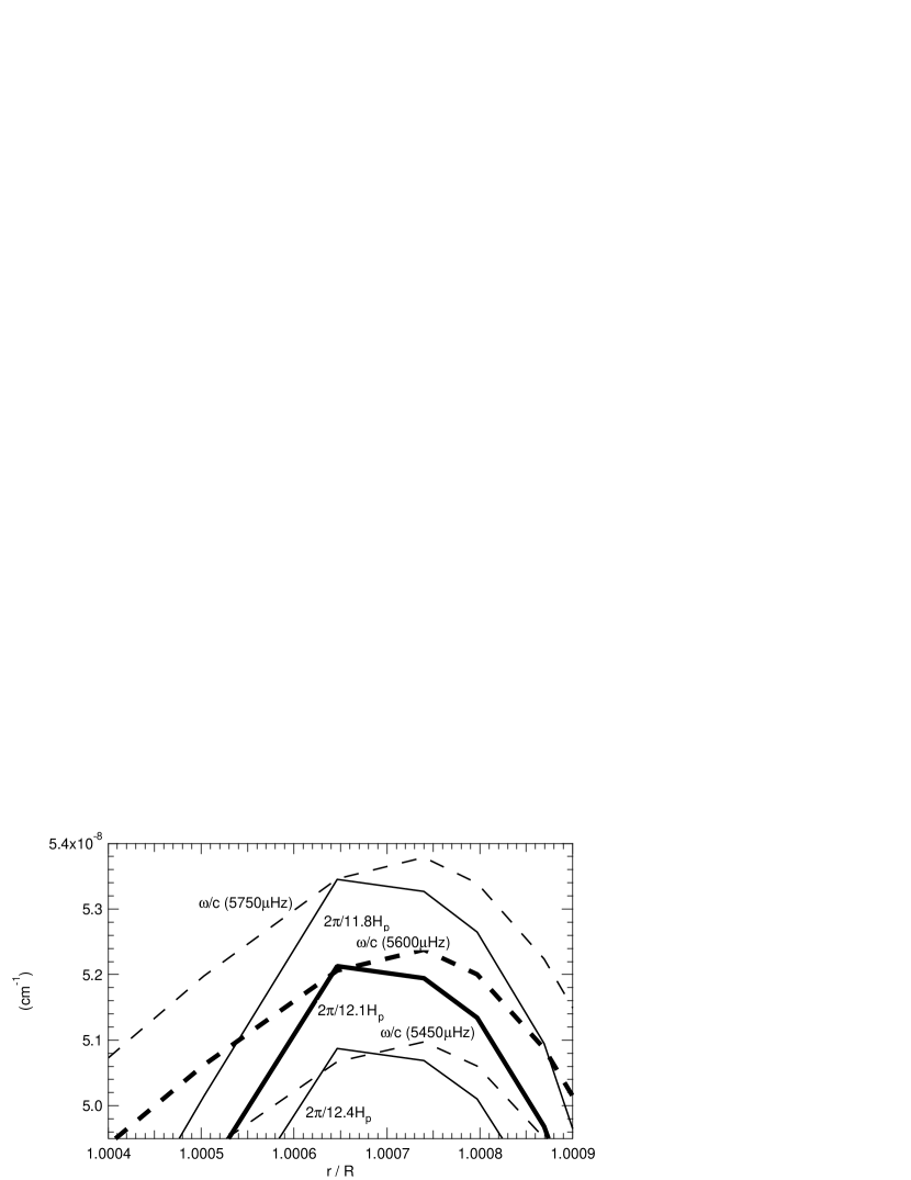
Figure 5: Determination of the coefficient $a_{v}$ in equation (35). Continuous curves: $2\pi/a_{v}H_{p}$ following the gaz pressure of the model C of Vernazza et al. (1981). Dashed curves: $\omega/c$. When $a_{v}=12.1$, the mode at 5600 $\mu$Hz is the last one trapped.

Figure 6: Some examples of external turning points determined by the intersection of the two curves expressed in equation (33): $k^{2}/k_{r}$ for $n=7$ and $l=0$, 1, 2, 3 (symbols described in fig.1 ), and $2\pi$/$12.1H_{p}$ (thick continuous line).

Conceptually speaking, the determination of the cavity external limit of a star is similar to that of a wind musical instrument with an open end. There, like for the Sun, one cavity end is not materially delimited while the eigenfrequencies are precisely defined. There also, the absence of an elaborate theory can be overcome by the use of experimental results to determine the equivalent external limits (Rayleigh, 1896, p. 201-202).

So all the external reflection conditions are defined.

In Figure 6 are given some examples of external turning points determined by the intersection of the two curves expressed in equation (33), for $l=0$, 1, 2, 3 and $n=7$. In such a diagram, the very low frequency modes $l=0$, 1 and $n=1$, 2 will have their representative curves under that of $2\pi/12.1H_{p}$ at several locations, which means that they hardly exist, the Sun structure being too inhomogeneous from their wavelength point of view.

2.6 Internal Turning Point ($l\neq 0$)

In the deep interior where the structure can be considered as locally homogeneous, there is no problem of boundary conditions and thus no genuine reflection point. (Except for some very low $l,n$ modes, see the section above, and for the $l=0$ modes, see the next section). Nevertheless, the spherical symmetry implies that there always exists an innermost point, called the internal turning point $r_{1}$, the location where the radial component of the wave vector vanishes. And, when studying only the radial part, we need to determine this internal turning point and the phase condition there. For non-radial modes, i.e. with $l$ and $k_{h}\neq 0$, $r_{1}$ is given by

$$k_{r}=0\Leftrightarrow\frac{c_{0}^{2}}{r_{1}^{2}}-\frac{4\pi G\rho_{0}}{l(l+1)}=\frac{\omega^{2}}{l(l+1)}.$$ (37)

When the gravitational contribution is neglected ($G\rho_{0}=0$), the expression (37) is reduced to the well known one used in the context of current asymptotic approximations

$$\frac{c_{0}^{2}}{r_{1}^{2}}=\frac{\omega^{2}}{l(l+1)}.$$ (38)

Some turning points can already be seen on Figure 6 where $1/k_{r}\rightarrow\infty$. It is also interesting to represent the right or left member of equation (37) as a function of the radius (Figure 7 for the Sun), so that $r_{1}$ can be immediately determined once the frequency and the degree of a mode are known. For a given $\omega$, the larger the degree, the less the mode goes deep. For a given degree, the larger the $\omega$, the deeper the mode goes. For the degrees $l\geq 5$, the curves begin to merge together with that where $G\rho_{0}=0$, which is independent of $l$. For the smaller degrees, the difference with the case without gravity is appreciable, even far from the centre, until the middle of the solar radius, because while $\rho_{0}$ decreases with the radius, $c_{0}^{2}/r^{2}$ decreases also quickly. The curve for the $l=1$ modes present a further special feature: the gravitation term becomes much more important compared to $c_{0}^{2}/r^{2}$, so that a gap appears in the radiative zone, separating the curve into 2 parts, and for the concerned frequencies, the outermost turning point $r_{1}/R$ is drastically reduced to 0.137 instead of 1 for the other degrees.

Figure 7: Right or left member of equation (37) and (65), as a function of radius. The cases of $l=0$, 1, 2, 3, in the presence of gravity (symbols as defined in Figure 1) are compared to the case without gravity (upper thick continuous line).

The turning points $r_{1}/R$ are given in Table 1 for different $l$ values at typical levels of $\omega^{2}/l(l+1)$, to be compared to the case without gravity to appreciate the contribution of gravity for the Sun.

Table 1: Internal turning points $r_{1}/R$ in the presence of gravity, for different $l$ at typical levels of $\omega^{2}/l(l+1)$, compared to the case without gravity.

$$\begin{array}[]{ccccc}\hline\cr&\frac{\omega^{2}}{l(l+1)}=&10^{-5}&\ \ \ 10^{-6}&3\,10^{-7}\\ \hline\cr l=1&&0.110&0.134&0.137\\ l=2&&0.168&0.388&0.621\\ l=5&&0.198&0.445&0.646\\ l=10&&0.203&0.452&0.650\\ \hline\cr Without\,G&&0.205&0.454&0.652\\ \end{array}$$

Globally, when the gravitational potential is taken into account, $r_{1}$ is smaller, especially for $l=1$. Gravity pulls the low $l$ modes toward the centre.

The location of the internal turning point can be directly determined by a mathematical expression, while the phase condition at this point is less easy to find out. A discussion about $H_{p}$ like at the surface is of no use because here its projection on the propagation direction vanishes. Let us come back to equation (13) governing $P^{\prime}=rp^{\prime}$, which admits the JWKB standing-wave solution

$$P^{\prime}(r)=\frac{2A}{\sqrt{k_{r}}}\cos\left(-\int_{r_{0}}^{r}\!\!k_{r}dr+\frac{\psi-\psi^{\prime}}{2}\right).$$ (39)

This solution fails of course near $r=r_{1}$ where $k_{r}=0$. A well known method to bypass this difficulty is to develop linearly $k_{r}^{2}$ around $r_{1}$

$$k_{r}^{2}=k_{1}(r-r_{1})$$ (40)

and to adopt a new variable $x$

$$x=k_{1}^{1/3}(r-r_{1})$$ (41)

where $k_{1}$ is the derivative of $k_{r}^{2}$ in $r_{1}$. Equation (13) becomes

$$\frac{d^{2}P^{\prime}}{dx^{2}}+xP^{\prime}=0$$ (42)

which admits the general solution

$$P^{\prime}=C\mbox{Ai}(-x)+D\mbox{Bi}(-x)$$ (43)

where $C$ and $D$ are the constants to be determined, Ai and Bi the Airy functions which present an undulatory behaviour for positive x and an exponential behaviour for negative x. As the Ai function is exponentially decreasing toward the center while the Bi function is increasing, one must choose $D=0$. The next step is to fit the two solutions (39) and (43) at a fit location $r_{f}$. This latter is usually chosen so that the corresponding $x_{f}$ is very large, in order to use the asymptotic development of Ai which is sinusoidal, and to deduce easily the wave phase. In fact, this method introduces an important lack of precision because the Airy solution is only valid when (40) is valid, that is around $x=0$. We will here adopt fitting points $r_{f}$ that are a priori not far from $r_{1}$, corresponding to small values of $x_{f}$. Consider now the standing solution coming from the nearest antinode to $r_{1}$, located at $r_{a}$, we have $(\psi-\psi^{\prime})/2=0$ in equation (39). When matching this solution and its derivative to the Airy solution at the the fitting point:

$$\frac{2A}{\sqrt{k_{r}}}\cos\int_{r_{a}}^{r_{f}}\!\!\!\!k_{r}dr=C\mbox{Ai}(-x_{f})$$ (44)

$$2A\sqrt{k_{r}}\sin\int_{r_{a}}^{r_{f}}\!\!\!\!k_{r}dr-Ak_{r}^{-3/2}\frac{dk_{r}}{dr}\cos\int_{r_{a}}^{r_{f}}\!\!\!\!k_{r}dr$$

$$\!\!\!\!\!\!\!\!\!\!\!=-C\mbox{Ai'}(-x_{f})k_{1}^{1/3}$$ (45)

the phase of the standing wave is imposed :

$$\int_{r_{a}}^{r_{f}}\!\!\!\!k_{r}dr=-\arctan\left[\frac{1}{4k_{r}^{3}}\frac{dk_{r}^{2}}{dr}-\frac{k_{1}^{1/3}}{k_{r}}\frac{\mbox{Ai'}(-x_{f})}{\mbox{Ai}(-x_{f})}\right]$$ (46)

where Ai’ stands for the derivative of Ai over $x$. As $\alpha$ is the phase lag between $r_{1}$ and a displacement antinode, i.e. a pressure node located in $r_{n}$, it is given by (see fig. 3)

$$\alpha\pi=-\int_{r_{n}}^{r_{1}}=-\int_{r_{n}}^{r_{a}}-\int_{r_{a}}^{r_{f}}-\int_{r_{f}}^{r_{1}}$$ (47)

where the terms $k_{r}dr$ inside the integral signs are implicit. This matching has only a sense when equation (40) can be used. Applying this latter and equation (41), then calculating the first and third integrals of equation (47), the final expression of $\alpha$ can be expressed as a function of $x_{f}$:

$$\alpha\pi=-\frac{\pi}{2}+\arctan\left\{\frac{1}{x_{f}^{0.5}}\left[\frac{1}{4x_{f}}-\frac{\mbox{Ai'}(-x_{f})}{\mbox{Ai}(-x_{f})}\right]\right\}+\frac{2}{3}x_{f}^{3/2}.$$ (48)

It remains now to determine the fitting point. It should be chosen at the farthest limit toward $r_{1}$ where the JWKB solution is still valid, to be also in the validation domain of the Airy solution. As seen in appendix A, the JWKB method is valid as long as the derivative of $k_{r}$ is enough small compared to $k_{r}$:

$$\frac{dk_{r}}{dr}\leq ak_{r}^{2}\Leftrightarrow\frac{1}{2k_{r}^{3}}\frac{dk_{r}^{2}}{dr}\leq a$$ (49)

where a is a ‘small’ number. In other words, the variation of $P^{\prime}$ must be slow enough on a wavelength when $k_{r}$ goes to zero. This condition should be coherent with that at the external limit which is of the same nature (eq. 1), except that the characteristic scale height $H_{f}$ to be considered here does not come from the environment but from the function $P^{\prime}$ itself. We can define a function f

$$f=\frac{1}{\sqrt{k_{r}}}$$ (50)

and should use the already determined coefficient $a_{v}$ to write the condition

$$\frac{2\pi}{k_{r}}\leq a_{v}H_{f}$$ (51)

with

$$H_{f}^{-1}=-\frac{1}{f}\frac{df}{dr}=\frac{1}{4k_{r}^{2}}\frac{dk_{r}^{2}}{dr}.$$ (52)

The searched condition (49) is thus

$$\frac{1}{2k_{r}^{3}}\frac{dk_{r}^{2}}{dr}\leq\frac{a_{v}}{\pi}.$$ (53)

Using equation (40), a first fitting point can then be obtained

$$r_{f1}=r_{1}+\frac{(\pi/2a_{v})^{2/3}}{k_{1}^{1/3}}.$$ (54)

Imposing that the ratio $k_{1}/k_{r}^{3}$ is enough small, the condition (53) is in fact not sufficient to warranty the validity of the standing wave solution. When $l$ and $n$ are small, the slope $k_{1}$ of the function $k_{r}^{2}$ can be so close to zero that $k_{r}^{2}$ will also remains very close to zero. The wave solution loose its meaning because the wavelength becomes too large. Either $k_{1}$ or $k_{r}^{2}$, or their product should be enough large. The smallest $k_{r}$ is determined by the largest wavelength that can be contained in the cavity:

$$\lambda_{r}\leq r_{2}-r_{1}\Rightarrow k_{r}\geq\frac{2\pi}{r_{2}-r_{1}}.$$ (55)

The smallest slope $k_{1}$ should be so that $k_{r}$ reaches an ‘appreciable’ value , let us say corresponding to $\lambda_{r}\leq r_{2}$, on a ‘negligible’ distance, i.e. a distance $(r-r_{1})$ small enough compared to the wavelength. To be coherent with above, we use again the coefficient $a_{v}$ and the relation (1) with the inverse inequality sign

$$\lambda=\frac{2\pi}{k_{r}}\geq a_{v}(r-r_{1}).$$ (56)

That leads to

$$k_{1}\geq a_{v}\frac{(2\pi)^{2}}{r_{2}^{3}}$$ (57)

which, together with equation (55) allow to arrive to the searched condition on the product $k_{1}k_{r}^{2}$

$$k_{1}k_{r}^{2}\geq a_{v}\frac{(2\pi)^{4}}{(r_{2}-r_{1})^{2}r_{2}^{3}}.$$ (58)

Using equation (40), the second fitting point can be obtained

$$r_{f2}=r_{1}+\frac{a_{v}(2\pi)^{4}}{(r_{2}-r_{1})^{2}r_{2}^{3}k_{1}^{2}}.$$ (59)

The final fitting point can be taken as a compromise between the conditions (53) and (58), that is a mean value between $r_{f1}$ and $r_{f2}$

$$r_{f}=r_{1}+\frac{(\pi/2a_{v})^{2/3}}{2k_{1}^{1/3}}+\frac{a_{v}(2\pi)^{4}}{2(r_{2}-r_{1})^{2}r_{2}^{3}k_{1}^{2}}.$$ (60)

Everything is now ready for the complete calculation of the $l\neq 0$ modes.

2.7 Internal Turning Point ($l=0$)

For the radial modes

$$l=0,\ k_{h}=0,\ k_{r}=k>0,$$ (61)

there is a priori no turning point as for $l\neq 0$. It is very tempting to conclude that these modes pass through the star center which is a node, since due to symmetrical reasons it must stay immobile. In this case:

$$r_{1}=0,\ and\ \alpha=-0.5.$$ (62)

But this induces eigenfrequencies that are lower than numerical or observed results by several tens of $\mu$Hz. In fact, no mode can touch the center: the linear solution of local wave cannot be applied at $r=0$. For a spherical wave, it is obvious that the center is a singular point according to its expression (31). The wave must be stopped somewhere before reaching the center. As the perturbed pressure $p^{\prime}$ goes to infinity, for the wave, everything happens as if the surrounding pressure goes to zero. And everything looks like the vacuum condition at the external limit, except that here the decreasing ‘external’ pressure is directly given by a law in $1/r$. Thus $H_{p}=r$, and the condition (1) gives the turning point $r_{1}$

$$k_{r}=\frac{2\pi}{a_{v}r}.$$ (63)

Taking into account the numerical value of $a_{v}$ (Eq. 36), this relation can be written as

$$\frac{\omega^{2}+4\pi G\rho_{0}}{c_{0}^{2}}-\frac{(0.51927)^{2}}{r_{1}^{2}}=0.$$ (64)

When neglecting the gravity, this formula is very close to that using by traditional approximations where the term $l(l+1)$ is artificially replaced by $(l+0.5)^{2}$. Therefore, the present concept of ‘vacuum condition’ characterised by the coefficient $a_{v}$, could be considered as the justification of this usual way of doing for $l=0$.

Equation (64) can also be rewritten in a general form like Equation (37):

$$\frac{c_{0}^{2}}{r_{1}^{2}}-\frac{4\pi G\rho_{0}}{(2\pi/a_{v})^{2}}=\frac{\omega^{2}}{(2\pi/a_{v})^{2}}$$ (65)

This expression is also represented in Figure 7 giving the internal turning point. The curve features an important gap in the radiative zone, even bigger than for the $l=1$ modes, and for the concerned frequencies the largest possible $r_{1}/R$ can only go up to 0.035.

The internal turning point being determined, let us examine the phase at this location. Whenever the gravity is neglected, we are in the same ‘vacuum’ type condition than at the external boundary (Eq. 2) : the standing wave will present a pressure node or a displacement antinode. Thus, in this case

$$\alpha=0.$$ (66)

In the presence of a gravity field, the condition (3) must be rather applied, which can be rewritten as

$$p^{\prime}(r_{1})+\rho_{0}\phi^{\prime}(r_{1})=0.$$ (67)

As $r_{1}$ is very near the center, the exact solution of $\phi^{\prime}$ must be used. Indeed, resulting from Poisson’s equation, the gravitational potential as well as its perturbation must remain always finite, even at the center. Going back to equation (11), and with $\phi^{\prime}=F^{\prime}/r$, the equation that has to be solved is

$$\frac{d^{2}F^{\prime}}{dr^{2}}-\frac{l(l+1)}{r^{2}}\Phi^{\prime}=-\frac{4\pi GP^{\prime}}{c_{0}^{2}}.$$ (68)

To the particular solution given by equation (15), must be added the homogeneous solution

$$F^{\prime}=Cr^{l+1}+\frac{D}{r^{l}}$$ (69)

with C, D the constants to be determined. In order to have a negligible gravitational potential at large radius, $C=0$ must be chosen. And for $l=0$, D must be chosen so that the general solution is

$$\Phi^{\prime}(r)=\frac{4\pi G}{c_{0}^{2}k^{2}}\frac{A}{r\sqrt{k}}\left[\cos\left(-\int_{0}^{r}\!\!kdr+\psi\right)-cos\psi\right].$$ (70)

This keeps $\phi^{\prime}$ finite at $r=0$. Equation (67) becomes, for the corresponding standing waves

$$\left(\frac{c_{0}^{2}k^{2}}{4\pi G\rho_{0}}+1\right)\cos\left(\int_{0}^{r_{1}}\!\!\!\!kdr+\frac{\psi-\psi^{\prime}}{2}\right)-\cos\left(\frac{\psi-\psi^{\prime}}{2}\right)=0.$$ (71)

Knowing that

$$\int_{0}^{r_{n}}\!\!\!\!-kdr+\frac{\psi-\psi^{\prime}}{2}=\frac{\pi}{2}$$ (72)

with $r_{n}$ the location of the closest node to $r_{1}$, and

$$\alpha\pi=-\int_{r_{n}}^{r_{1}}=\int_{0}^{r_{n}}-\int_{0}^{r_{1}}$$ (73)

where the terms $kdr$ inside the integral signs are implicit, the equation determining $\alpha\pi$ can be deduced

$$\left(\frac{\omega^{2}}{4\pi G\rho_{0}}+2\right)\sin\alpha\pi-\sin\left(\alpha\pi+\int_{0}^{r_{1}}\!\!\!\!kdr\right)=0.$$ (74)

As generally $\alpha\pi\ll 1$, this can be simplified to:

$$\alpha\pi=\frac{\sin\int_{0}^{r_{1}}\!\!kdr}{\omega^{2}/4\pi G\rho_{0}+2-\cos\int_{0}^{r_{1}}\!\!kdr}.$$ (75)

As very near the center the wave number $k$ can be considered to be roughly constant,

$$\int_{0}^{r_{1}}\!\!\!\!kdr\simeq kr_{1}=\frac{2\pi}{a_{v}}$$ (76)

a further simplified expression for $\alpha$ can be used

$$\alpha\pi=\frac{\sin\frac{2\pi}{a_{v}}}{\frac{\omega^{2}}{4\pi G\rho_{0}}+2-\cos\frac{2\pi}{a_{v}}}.$$ (77)

When the gravity potential is neglected ($G\rho_{0}\rightarrow 0$), this expression is coherent with equation (66).

3 The Whole Set of Equations and Results

We have now every ingredient to calculate the eigenfrequencies. It is worth gathering here the whole set of equations used for the general case in the presence of gravity. Given the 2 parameters $l$, $n$ which are respectively the mode degree and order, a system of 2 equations with 2 unknowns $\omega$ and $\alpha$ has to be solved:

$$\!\!\!\!\!\int_{r_{1}}^{r_{2}}\!\!k_{r}dr=(n+\alpha)\pi$$ (78)

and for $l\neq 0$

$$\alpha\pi=-\frac{\pi}{2}+\arctan\left\{\frac{1}{x_{f}^{0.5}}\left[\frac{1}{4x_{f}}-\frac{\mbox{Ai'}(-x_{f})}{\mbox{Ai}(-x_{f})}\right]\right\}+\frac{2}{3}x_{f}^{3/2}$$ (79)

for $l=0$

$$\alpha\pi=\frac{\sin\frac{2\pi}{a_{v}}}{\frac{\omega^{2}}{4\pi G\rho_{0}}+2-\cos\frac{2\pi}{a_{v}}}$$ (80)

with

$$k_{r}=\sqrt{\frac{\omega^{2}+4\pi G\rho_{0}}{c_{0}^{2}}-\frac{l(l+1)}{r^{2}}}.$$ (81)

$r_{1}$ is given by

$$\!\!\!\!k_{r}=0\ \ for\ l\neq 0,\ \ \ k_{r}=\frac{2\pi}{a_{v}r}\ \ for\ l=0,$$ (82)

and $r_{2}$ given by

$$\frac{k^{2}}{k_{r}}=\frac{2\pi}{a_{v}H_{p}}$$ (83)

with

$$a_{v}=12.1.$$ (84)

$x_{f}$ is given by

$$x_{f}=k_{1}^{1/3}(r_{f}-r_{1})$$ (85)

where $k_{1}$ is the derivative of $k_{r}^{2}$ at $r_{1}$, and $r_{f}$ is given by

$$r_{f}=r_{1}+\frac{(\pi/2a_{v})^{2/3}}{2k_{1}^{1/3}}+\frac{a_{v}(2\pi)^{4}}{2(r_{2}-r_{1})^{2}r_{2}^{3}k_{1}^{2}}.$$ (86)

Equations (78-86) are the only equations needed for the frequency determination. This shows the simplicity of the present approach. Three functions of the equilibrium structure are directly involved, $c_{0}(r)$, $\rho_{0}(r)$ and $H_{p}(r)$. $H_{p}(r)$ is in fact only important at the surface in the determination of $r_{2}$. $\rho_{0}(r)$ contributes via the gravitational potential, which plays a crucial role toward the center, being more important for lower degree modes.

One can also notice the presence of the coefficient $a_{v}$ at external as wel as internal limit conditions. Determined initially by a ‘vacuum’ condition at the surface, it turns to play a key role in the study of the validity of the JWKB solution in general.

The above equations are obtained without neglecting the gravity effect. The induced results in the following sections will thus present the same quality at low as well as at large degree or order, except when deliberately ignoring the gravity term.

In the following, the results obtained with the above equations are exposed and commented, for the modes $l=0$ to 10, and frequencies in the range 300 - 5600 $\mu$Hz, firstly for the case without gravity, and secondly in the general case taken into account the gravity.

3.1 Results in the Case Without Gravity

Although neglecting the gravity is a crude approximation, it is very instructive because the corresponding physical conditions look like those of acoustic waves on Earth, which appear more familiar to us. Furthermore, that will allow direct comparisons with the existing semi-analytical approaches where the gravity effect is neglected or treated at the second order.

We employ the equations (78-86) with $G\rho_{0}\rightarrow 0$. The results are displayed in Figure 8 for the turning points $r_{1}$, $r_{2}$, the phase shift $\alpha$ and the difference $\nu-\nu_{num}$ between the eigenfrequencies resulting from the present work and those computed numerically (The numerical calculation automatically takes into account perturbation on gravity).

Figure 8: Case without gravity. Turning points, phases and frequencies for the modes $l=0$ to 10, compared to numerical frequencies where the gravity perturbation is taken into account. The symbols are defined in Figure 1.

The phase shift $\alpha$ lies in the range [-0.25, 0]. All the radial modes have the same $\alpha=0$, expressing the presence of a ‘vacuum pressure’. The non-radial modes have a common $\alpha$ value only at large frequencies. Indeed, for these latter, when $k_{1}$, the slope of $k_{r}^{2}$ ar $r_{1}$, is enough large, the last part of equation (86) is ngligible compared to the second one, and equation (79) gives a constant value for $\alpha$

$$\alpha=-0.0334$$ (87)

which is independent of $l$ and $n$.

The curves representing the inner turning points $r_{1}$ can be compared to those presented in Lopes & Turck-Chièze (1994), obtained from solar observed modes (Libbrecht et al., 1990), with a formalism using $L=(l+0.5)^{2}$. While given by diffferent formulas, the $r_{1}$ of radial and non-radial modes seem to be very similar.

The outer turning points $r_{2}$ feature a remarkable behaviour: for frequencies beyond 800 $\mu$Hz, $r_{2}$ depends very few on the mode order $l$ and much more on frequency. Indeed, equations (81) and (83) show that for low $l$, $k_{r}$ and $r_{2}$ are independent of $l$. That means that a modification of the Sun surface will modify in the same way all the modes of different degree. This fact will be exploited hereafter. This set of very grouped curves represents the external profile of the Sun acoustic cavity. One can also remark that $r_{2}$ increases very quickly with frequency, right beyond 2500 $\mu$Hz, its curve reaches already the flatten part, very close to $r_{2}/R=1$. The results from 1000 $\mu$Hz can be compared to the curve obtained by Deubner & Gough (1984) (and detailed in Christensen-Dalsgaard (1998)), following a general asymptotic expression obtained after several variable changes. One has otherwise keep in mind that:

1. Confusing $r_{2}$ with $R$ leads to frequency displacements of tens of $\mu$Hz.

2. For larger mode degrees, $r_{2}$ depends of course stronger on $l$ following equation (83).

Concerning the comparison to numerical results for the eigenfrequencies, a first observation of these raw data leads to a rather disappointing report: the differences reach -32/+60 $\mu$Hz. But a more detailed analysis shows that the differences to be taken into account are much smaller. Actually, these discrepancies consist mainly in a global undulation independent of $l$, signature of a difference, solely at the surface, between the two calculations. As justified in the next sections, a simple correction of surface conditions to be in accordance with the numerical code will cancel this undulation. Therefore only the thickness of the set of these curves is to be taken into account. Straight away then, the classical asymptotic character clearly appears, the differences being progressively bigger when the frequencies go lower, according to the importance of $G\rho_{0}$ in the expression of $k_{r}$ (eq. 81). By discarding the results at very low frequencies where the coupling with gravity modes can no more be neglected, in all the rest between 800 and 5100 $\mu$Hz, the differences are reduced to no more than $\pm 34\mu$Hz to $\pm 4\mu$Hz. Although having different $r_{1}$ and $\alpha$, the radial modes present differences with numerical results which are in continuity with the non-radial ones.

3.2 Results in the General Gase (With Gravity)

We use the set of equations (78-86) as they are. The results are displayed in Figure 9.

The external turning points $r_{2}$ are the same than without gravity because the gravity does not play any role at the surface. Every related comment in the previous section remains totally valid here.

As foreseen, the internal turning points $r_{1}$ are especially smaller for low-degree, low-frequency modes, the gravity acts like if it pulls these modes toward the centre. So the realted $\alpha$, which depends on $r_{1}$, is smaller in absolute value. These features are particularly noticeable for the $l=0$ and $l=1$ modes. The common value of $\alpha$ at large frequency, $\alpha$=-0.0334, remains the same. The $\alpha$ of the radial modes are now completely different, and are the only ones that are positive.

These different $r_{1}$ and $\alpha$, together with different $k_{r}$ in the inner parts will induce different eigenfrequencies when gravity is taken into account. One can moreover predict that all the frequencies will be lowered. These differences are larger for lower degree or higher frequency modes which travel deeper. To appreciate that numerically, some examples of frequencies without or with gravity, are given in Table 2 for various degrees and orders. The same type of comparison for $r_{1}$ was given in Table 1.

Table 2: Frequencies in $\mu$Hz without / with gravity, for various degrees and orders.

$\begin{array}[]{lccc}\hline\cr&n=2&n=10&n=30\\ \hline\cr l=0&453.2/363.7&\ \ 1570.1/1531.7&4291.8/4273.6\\ l=1&469.6/427.4&\ \ 1629.0/1591.3&4360.7/4340.8\\ l=2&512.2/492.7&1680.9/1655.6&4427.7/4410.0\\ l=5&622.1/618.8&1810.9/1801.8&4601.3/4590.5\\ l=10&767.3/766.4&1998.5/1995.7&4840.9/4835.4\\ \hline\cr\end{array}$

Figure 9: General case in the presence of gravity. Turning points, phases and frequencies for the modes $l=0$ to 10. The symbols are defined in Figure 1.

The curves of Figure 9 featuring the difference with numerical calculation show the same global undulation independent of $l$, at exactly the same locations in radius than with the case without gravity. For the same reason, only the thickness of this set of curves is to be considered. One can then conclude that between 800 and 5100 $\mu$Hz, the discrepancy is drastically reduced to within $\pm$ 3 $\mu$Hz. And the most remarquable point is that the former asymptotic behaviour when the gravity was neglected, has disappeared. Even radial and non-radial modes, which are governed by different physics of internal boundary condition, present the same profiles. This can lead to attribute a higher degree of confidence to the present calculations in general, and to the coefficient $a_{v}$ in particular.

3.3 Discussion on the Outer Boundary Conditions

The gravity being taken into account, it is now worth examining the global undulation independent of $l$ (Fig. 9) characterising the frequency differences with numerical results. As the solar model used is the same, that points out a difference in the external boundary conditions used in the two frequency calculations: the present semi-analytical calculation applies the condition of local inhomogeneity, while the numerical code is run with the isothermal atmosphere approximation.

Although the isothermal atmosphere approximation leads to frequencies that are closer to observations, several non-satisfying points remain:

• It is not very realistics, at least when compared to a semi-empirical atmosphere of the type of Vernazza et al. (1981), which presents no place with a flat temperature profile. No atmosphere coming from a stellar evolution code presents any more such a behaviour at the surface.

• It is not really physics, because an infinite isothermal atmosphere needs to be invoked, whose integrated mass is infinite.

• It requires to adjust a particular atmosphere to the input stellar model, thus actually changes the initial surface conditions of the latter. When discrepancies with observations are detected, it is not possible to distinguish the part coming from the initial surface conditions, and the part coming from its change by the adjustment of an isothermal atmosphere.

A search for boundary conditions using directly the input stellar structure without any modification, may be desirable. Then, any difference between two sets of frequencies could be attributed to differences in the stellar structures considered. The condition proposed here (eq. 83) is only a suggestion in this direction, which potentially allows to recover surface properties. To prove that, we can try here to find out the amosphere properties used by numerical calculation. As the wave solution is adjusted to that of the analytical solution in an infinite isothermal atmosphere adjusted to the initial atmosphere, this double adjustment amounts to modify very deeply the profiles of $\Gamma_{1}$ and $H_{p}$ while keeping unchanged their product. So the wave propagation is not affected, only its outer reflexion is concerned. Therefore we have to find out the $H_{p}$ change that cancel the frequency discrepancies. In our case, this is simple to do because there is a one-to-one correspondence between $\nu$ and $r_{2}$ (upper right panel of Fig. 9) and between $r_{2}$ and $H_{p}$ (Fig. 6), thus between $\nu$ and $H_{p}$. The result is shown in Fig. 10. In Nghiem (2003b), it was demonstrated that this profile is actually the $H_{p}$ profile when the procedure of isothermal atmosphere adjustment is performed. This profile does not have any consistency with the stellar structure because it results from a fit with a structure having very different properties.

With this deduced $H_{p}$ profile, the final frequency discrepancy is shown in Fig. 11. It remains large only for low frequencies $<$ 800 $\mu$Hz, where coupling with gravity modes is no more negligible. For frequencies between 800 and 5100 $\mu$Hz, the discrepancy is on the contrary reduced as expected to less than $\pm 3\mu$Hz.

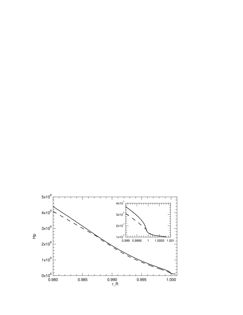
Figure 10: Profiles of the pressure scale height at the surface and zoom at the external limit. Continuous line: initial $H_{p}$ coming from the stellar evolution code. Dashed-line: $H_{p}$ expected to come from the double adjustment of the isothermal atmosphere approximation.

Figure 11: Resulting frequency discrepancy with numerical results for the modes $l=0$ to 10, in the presence of the $H_{p}$ profile expected to come from the isothermal atmosphere approximation (Fig. 10). The symbols are defined in Fig. 1.

4 Comparison With Observations

Fig 12 gives the differences between frequencies obtained by the present study on the solar structure coming from the evolution code, and those obtained by solar observations coming from the SoHO spacecraft. There is a global modulation independent of $l$ like with numerical results but different in values, going down to -40 $\mu$Hz, and up to +30 $\mu$Hz. This comes indisputably from problems at the surface, and can be attributed to the fact that the solar model used does not yet take into account some important physical phenomenon. In Nghiem et al. (2004) it was assumed that it concerns exclusively a magnetic field, which modifies the structure by the magnetic pressure and the Alfven speed. Then we aim to search for perturbed pressure and sound speed profiles that cancel the frequency discrepancies. The results are shown in Figure 13. That finally allows to obtain the frequency differences of only $\pm 2\mu$Hz in the whole studied frequency range (Fig. 14). In the same way, a magnetic variation has also been calculated to account for the frequency variation related to the solar cycle. But this study has to be confirmed by a more detailed one, especially by taking into account the density change with the introduction of the magnetic field.

These results does not exclude that other usual phenomena (turbulent pressure, non-adiabaticity, etc.) can reduce the theory-observation discrepancy in frequencies. Thay have only shown the capabilities of the proposed method to recover identified surface properties, because no a-priori hypothesis was made on the structure. If numerical codes can adopt the same type of boundary conditions than here, absolute frequency values could be calculated at a precision well better than $\pm 1\mu$Hz in the whole frequency range. That will be very helpful for asteroseismology in the identification of the modes, when only very few low-order frequencies will be available.

Figure 12: Frequency differences with observational data for the modes $l=0$ to 10. The symbols are defined in Fig. 1.

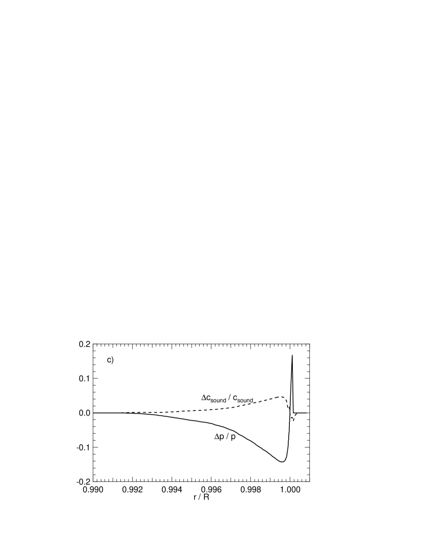
Figure 13: Profiles at the surface of the pressure and sound speed changes, expected to come from a magnetic field, which cancel discrepancies with observational frequencies.

Figure 14: Resulting frequency discrepancies with observational data for the modes $l=1$ to 10, after the changes of pressure and sound speed in Fig. 13. The symbols are defined in Fig. 1.

5 Conclusions-Discussions

The local wave approximation has been fully and coherently applied to stellar acoustic modes. Conceptually, it is in total accordance with the JWKB approach. Pratically, it consists in clearly determining the cavity limits and the reflection conditions. The standing wave nature of the modes are thus firmly claimed. In this simple context, a particularly reduced number of equations is necessary.

The wave propagation in the innner part is nevertheless correctly represented, as the gravity effect is directly taken into account. No development into higher orders, no artificial change of the horizontal eigenvalue $l(l+1)$ are needed. It turns out that the $l=0$ modes do not touch the centre. Not surprisingly, the gravity plays an important role for low-$l$ modes, being able to shift frequencies by tens of $\mu$Hz. The main result is that the present analytical calculation is equally valid for low than high frequencies and degrees, only the coupling with gravity modes is not considered.

At the surface, a new boundary condition is proposed, directly based on the propagation condition of an acoustic wave, which corresponds to the JWKB validity criteria. Although that returning point should perhaps be refined, some first conclusions can already be drawn. A coefficient like $a_{v}$ seems to be sufficient to characterize the validity of a JWKB solution. But the main result is that an alternating boundary condition leads to frequency shifts of the same range than present theory-observation discrepancies. To explain the latter, a search for a more appropriate boundary condition cannot be excluded. The method proposed here has the advantage to use the atmosphere model as it is, without any modification. Comparisons with observations should allow to directly recover the real atmosphere structure. Examples are given to find out the atmosphere used by numerical codes in the context of isothermal atmosphere approximation, and to suggest a way to deduce physical properties of the solar atmosphere when observations are considered.

Despite the simplicity of the proposed semi-analytical formalism, it seems that main physical phenomenons involved are taken into account. That is why for the Sun, a precision of $\pm 3\mu$Hz can be reached in the range 800-5600 $\mu$Hz, and for $l=0-10$. Some calculations for other stars show a comparable behaviour. If now a similar type of external boundary conditions is used in numerical calculations, a potential precision well better than 1$\mu$Hz can be expected for the whole frequency range. That could represent a step forward a global agreement between the three actors involved in helio-, astero-seismology: semi-analytical calculation bringing the physical understanding by predicting the good trend for the results, numerical calculation bringing the high precision by avoiding most of the approximations, and observation allowing to infer real stellar structures when searching to cancel theory-observation discrepancies.

Appendix A The JWKB Approach

Only a brief recall of the JWKB method is proposed here, detailed historical and theoretical considerations are out of this paper frame. The reader can see e.g. Elmore & Heald (1969). Let $y$ be the unknown function of the variable $r$ ruled by the propagation equation

$$\frac{d^{2}y}{dr^{2}}+k_{r}^{2}y=0$$ (A1)

with $k_{r}$ a constant. The solution is of course the wave function:

$$y=A\exp(\pm ik_{r}r)$$ (A2)

with A an arbitrary constant. Consider now the case where $k_{r}$ is itself a function of $r$, the equation

$$\frac{d^{2}y}{dr^{2}}+k_{r}^{2}(r)y=0$$ (A3)

admits no known solution in the general case, and certainly no wave solution like equation (A2). A complex solution of the type

$$y=A(r)\exp[iS(r)]$$ (A4)

can be tried, with A, S functions of $r$. By separating real and imaginary parts, one obtains:

$$A = CS^{\prime-1/2}$$ (A5)

$$S^{\prime 2} = k_{r}^{2}-\frac{1}{2}\frac{S^{\prime\prime\prime}}{S^{\prime}}+\frac{3}{4}\frac{S^{\prime\prime 2}}{S^{\prime 2}}$$ (A6)

where $S^{\prime},S^{\prime\prime},S^{\prime\prime\prime}$ stands for the successsive derivatives of $S$. When $S^{\prime\prime\prime}$ and $S^{\prime\prime}$ are negligible compared to $S^{\prime}$,

$$\frac{S^{\prime\prime 2}}{S^{\prime 2}}<<k_{r}^{2}\ \ \ \ and\ \ \ \frac{S^{\prime\prime\prime}}{S^{\prime}}<<k_{r}^{2}$$ (A7)

and only in that case, equation (A6) can be simplified to

$$S^{\prime}=\pm k_{r}$$ (A8)

and one has a wave-like solution:

$$y=\frac{C}{\sqrt{k_{r}}}\exp\left(\pm i\int\!\!k_{r}dr\right)$$ (A9)

with C an arbitrary constant.

Appendix B Eigenfunction, Radial Density of Kinetic Energy, and $k_{r}$

There is sometimes a confusion between the eigenfunction and the radial density of kinetic energy, or related quantities… Let us first of all precise that here the eigenfunctions are of the type $y(r)$ given by Eq. (31), where $y$ stands either for $\rho^{\prime}$, $p^{\prime}$, $\phi^{\prime}$, or $\xi_{r}$.

The amplitudes $A/r$ remain to be determined. It can be done in the context of the JWKB approximation (eq. A9), but that is not enough detailed because some slowly varying terms can still be contained in the ‘constant’ amplitude that is infact slowly variable itself. For $\xi_{r}$ for example, physical considerations about kinetic energy allow to have a more detailed determination of the amplitude. For a locally plane wave, the kinetic energy integrated in each wavelength (one spatial oscillation) is the same. So the kinetic energy per unit length is proportional to the number of wavelengths per unit length, i. e. the wavenumber:

$$\frac{\partial E_{k}}{\partial s}\propto k$$ (B1)

where s is the curviligne coordinate following the wave trajectory. Now for the motion of a locally spherical wave projected on the radial direction, the quantity that is conserved and proportional to $k_{r}$ is the radial kinetic energy per unit of radius, or if one prefers, its flux over any sphere of radius $r$:

$$\frac{\partial\epsilon_{k}}{\partial r}=\frac{1}{2}\rho_{0}\left(\frac{\partial\xi_{r}}{\partial t}\right)^{2}r^{2}=\frac{\omega^{2}}{2}\rho_{0}\xi_{r}^{2}r^{2}\propto k_{r}$$ (B2)

So the amplitude of $\xi_{r}$ is proportional to

$$\xi_{r}\propto\frac{\sqrt{k_{r}}}{r\omega\sqrt{\rho_{0}}}.$$ (B3)

That is the reason why sometimes $r\sqrt{\rho_{0}}\,\xi_{r}$ is called the ‘eigenfunction’, which is in fact proportional to the square root of $\partial\epsilon_{k}/\partial r$. Figures 15 show that this quantity is well proportional to $\sqrt{k_{r}}$. Some other times, that is rather $r\sqrt{\rho_{0}c_{0}}\,\xi_{r}$ which is called the ‘eigenfunction’, and this function has consequently a constant amplitude along $r$.

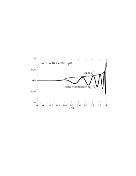
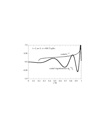
Figure 15: Scaled $k_{r}^{1/2}$ (dashed-line) superimposed on scaled ‘eigenfunctions’ (continuous line) coming from the numerical code, for three different cases of $l$, $n$.

References

- Bertello et al. (2000) Bertello, L., Henney, C. J., Ulrich, R. K., Varadi, F., Kosovichev, A. G., Scherrer, P. H., Cortés, T. R., Thiery, S., Boumier, P., Gabriel, A. H., & Turck-Chièze, S. 2000, ApJ, 535, 1066
- Christensen-Dalsgaard (1982) Christensen-Dalsgaard, J. 1982, MNRAS, 199, 735
-
Christensen-Dalsgaard (1997)
—. 1997, Notes on adiabatic oscillation programme,
http://www.obs.aau.dk/~jcd/adipack.n/ -
Christensen-Dalsgaard (1998)
—. 1998, Lecture Notes on Stellar Oscillations, 4th edition,
http://www.obs.aau.dk/~jcd/oscillnotes/ - Christensen-Dalsgaard & Berthomieu (1991) Christensen-Dalsgaard, J., & Berthomieu, G. 1991, Theory of solar oscillations, in Solar interior and atmosphere (ed. Cox, A. N., Livingston, W. C. & Matthews, M. S.; Tucson, AZ: University of Arizona Press), 401
- Couvidat et al. (2003) Couvidat, S., Turck-Chièze, S., & Kosovichev, A. G. 2003, ApJ, 599, 1434
- Cowling (1941) Cowling, T. G. 1941, MNRAS, 101, 367
- Cox (1980) Cox, J. P. 1980, Theory of stellar pulsation (Princeton, NJ: Princeton University Press)
- Deubner & Gough (1984) Deubner, F., & Gough, D. 1984, ARA&A, 22, 593
- Duvall (1982) Duvall, T. L. 1982, Nature, 300, 242
- Dzhalilov et al. (2000) Dzhalilov, N. S., Staude, J., & Arlt, K. 2000, A&A, 361, 1127
- Elmore & Heald (1969) Elmore, W. C., & Heald, M. A. 1969, Physics of waves (Toronto: General Publishing Company, 1969)
- Fossat et al. (1992) Fossat, E., Regulo, C., Roca Cortes, T., Ekhgamberdiev, S., Gelly, B., Grec, G., Khalikov, S., Khamitov, I., Lazrek, M., & Palle, P. I. 1992, A&A, 266, 532
- García et al. (1998) García, R. A., Pallé, P. L., Turck-Chièze, S., Osaki, Y., Shibahashi, H., Jeffries, S. M., Boumier, P., Gabriel, A. H., Grec, G., Robillot, J. M., Roca Cortes, T., & Ulrich, R. K. 1998, ApJ, 504, L51
- García et al. (2001) García, R. A., Régulo, C., Turck-Chièze, S., Bertello, L., Kosovichev, A. G., Brun, A. S., Couvidat, S., Henney, C. J., Lazrek, M., Ulrich, R. K., & Varadi, F. 2001, Sol. Phys., 200, 361
- Kosovichev (1995) Kosovichev, A. G. 1995, in Proc. of Fourth SOHO Workshop, ESA SP-376, Helioseismology, ed. J. T. Hoeksema, V. Domingo, B. Fleck, & B. Battrick (Noordwijk: ESA Publications Division), 165
- Lamb (1909) Lamb, H. 1909, in Proc. of London Math. Soc., vol. 7, 122
- Lamb (1932) Lamb, H. 1932, Hydrodynamics (New York: Dover)
- Langer (1937) Langer, R. E. 1937, Physical Review, 51, 669
- Leibacher & Stein (1981) Leibacher, J. W., & Stein, R. F. 1981, in The Sun as a Star, NASA SP-450, ed. S. Jordan, 263
- Libbrecht et al. (1990) Libbrecht, K. G., Woodard, M. F., & Kaufman, J. M. 1990, ApJS, 74, 1129
- Lopes & Turck-Chièze (1994) Lopes, I., & Turck-Chièze, S. 1994, A&A, 290, 845
- Morel (1997) Morel, P. 1997, A&AS, 124, 597
- Nghiem (2000) Nghiem, P. A. P. 2000, in Proc. of SOHO10/GONG2000 Workshop, ESA SP-464, Helio- and Astero- seismology at the dawn of the millenium, ed. A. Wilson (Noordwijk: ESA Publications Division), 665, tenerife, Spain
- Nghiem (2003a) Nghiem, P. A. P. 2003a, in Proc. of SOHO12/GONG+2002 Workshop, ESA SP-517, Local and Global Helioseismology: the Present and Future, ed. H. Sawaya-Lacoste (Noordwijk: ESA Publications Division), 155
- Nghiem (2003b) Nghiem, P. A. P. 2003b, in Proc. of SOHO12/GONG+2002 Workshop, ESA SP-517, Local and Global Helioseismology: the Present and Future, ed. H. Sawaya-Lacoste (Noordwijk: ESA Publications Division), 353
- Nghiem et al. (2004) Nghiem, P. A. P., García, R. A., Turck-Chièze, S., & Jimeénez-Reyes, S. J. 2004, in Proc. of SOHO14/GONG2004 Workshop, ESA SP-559, Helio- and Asteroseismology: Towards a Golden Future, ed. D. Danesy (Noordwijk: ESA Publications Division), 577
- Rayleigh (1896) Rayleigh, J. W. 1896, Theory of sound, 2nd ed., Vol. 2 (New York: Macmillan and Co., Ltd.)
- Rhodes et al. (1997) Rhodes, E. J., Kosovichev, A. G., Schou, J., Scherrer, P. H., & Reiter, J. 1997, Sol. Phys., 175, 287
- Rosenthal et al. (1995) Rosenthal, C. S., Christensen-Dalsgaard, J., Houdek, G., Monteiro, M., Nordlund, Å., & Trampedach, R. 1995, in Proc. of Fourth SOHO Workshop, ESA SP-376, Helioseismology, ed. J. T. Hoeksema, V. Domingo, B. Fleck, & B. Battrick (Noordwijk: ESA Publications Division), 459P
- Rosenthal et al. (1999) Rosenthal, C. S., Christensen-Dalsgaard, J., Nordlund, Å., Stein, R. F., & Trampedach, R. 1999, A&A, 351, 689
- Roxburgh & Vorontsov (2000) Roxburgh, I. W., & Vorontsov, S. V. 2000, MNRAS, 317, 141
- Tassoul (1980) Tassoul, M. 1980, ApJS, 43, 469
- Turck-Chièze et al. (2001) Turck-Chièze, S., Couvidat, S., Kosovichev, A. G., Gabriel, A. H., Berthomieu, G., Brun, A. S., Christensen-Dalsgaard, J., García, R. A., Gough, D. O., Provost, J., Roca-Cortes, T., Roxburgh, I. W., & Ulrich, R. K. 2001, ApJ, 555, L69
- Turck-Chièze et al. (1993) Turck-Chièze, S., Däppen, W., Fossat, E., Provost, J., Schatzman, E., & Vignaud, D. 1993, Phys. Rep., 230, 57
- Unno et al. (1989) Unno, W., Osaki, Y., Ando, H., Saio, H., & Shibahashi, H. 1989, Nonradial oscillations of stars (New York: Tokyo: University of Tokyo Press, 1989, 2nd ed.)
- Vanlommel & Goossens (1999) Vanlommel, P., & Goossens, M. 1999, Sol. Phys., 187, 357
- Vernazza et al. (1981) Vernazza, J. E., Avrett, E. H., & Loeser, R. 1981, ApJS, 45, 635
- Vorontsov (1991) Vorontsov, S. V. 1991, Soviet Ast., 35, 400
- Wright & Thompson (1992) Wright, A. N., & Thompson, M. J. 1992, A&A, 264, 701