Simulation of Coherent Nonlinear Neutrino Flavor Transformation
in the Supernova Environment: Correlated Neutrino Trajectories

Abstract

We present results of large-scale numerical simulations of the evolution of neutrino and antineutrino flavors in the region above the late-time post-supernova-explosion proto-neutron star. Our calculations are the first to allow explicit flavor evolution histories on different neutrino trajectories and to self-consistently couple flavor development on these trajectories through forward scattering-induced quantum coupling. Employing the atmospheric-scale neutrino mass-squared difference ($|\delta m^{2}|\simeq 3\times 10^{-3}\,\mathrm{eV}^{2}$) and values of $\theta_{13}$ allowed by current bounds, we find transformation of neutrino and antineutrino flavors over broad ranges of energy and luminosity in roughly the “bi-polar” collective mode. We find that this large-scale flavor conversion, largely driven by the flavor off-diagonal neutrino-neutrino forward scattering potential, sets in much closer to the proto-neutron star than simple estimates based on flavor-diagonal potentials and Mikheyev-Smirnov-Wolfenstein evolution would indicate. In turn, this suggests that models of r-process nucleosynthesis sited in the neutrino-driven wind could be affected substantially by active-active neutrino flavor mixing, even with the small measured neutrino mass-squared differences.

I Introduction

In this paper we employ large-scale computational techniques to tackle the vexing problem of neutrino flavor transformation in the core collapse supernova environment. Neutrinos and the weak interaction play pivotal roles in the core collapse/explosion phenomenon. The Chandrasekhar mass core of iron-peak material left at the end of the hydrostatic evolution of a massive star goes dynamically unstable and collapses in $\sim 1$ s to a proto-neutron star configuration at nuclear density. The amount of gravitational energy promptly converted into trapped seas of neutrinos is $\sim 1\%$ ($\sim 10^{52}$ erg) of the core mass. Within a few seconds after bounce $\sim 10\%$ ($\sim 10^{53}$ erg) of the core mass (the gravitational binding energy) will be emitted as neutrinos.

Nearly all of this gravitational energy is converted into seas of $\nu_{e}$, $\bar{\nu}_{e}$, $\nu_{\mu}$, $\bar{\nu}_{\mu}$, $\nu_{\tau}$ and $\bar{\nu}_{\tau}$ neutrinos in rough energy equipartition. Though these neutrinos diffuse with short mean free paths in the proto-neutron star, they decouple near the stellar surface where the matter density falls off steeply, the so-called neutrino sphere. Neutrinos propagate nearly coherently above this point, though neutrino-matter interactions, especially the charged current capture reactions $\nu_{e}+n\rightarrow p+e^{-}$ and $\bar{\nu}_{e}+p\rightarrow n+e^{+}$, can deposit energy and set the local neutron-to-proton ratio, $n/p$.

For this reason, and because the fluxes and energy spectra may be different for $\nu_{e}$, $\bar{\nu}_{e}$ and $\nu_{\mu}\bar{\nu}_{\mu}\nu_{\tau}\bar{\nu}_{\tau}$, the flavor content of the neutrino field above the proto-neutron star and its evolution in time and space can be important Fuller et al. (1992); Qian et al. (1993); Qian and Fuller (1995a). This can be true both for the supernova shock reheating epoch (where the time post core-bounce is $t_{\mathrm{PB}}\lesssim 0.5$ s) and in the later hot bubble, neutrino-driven wind epoch ($t_{\mathrm{PB}}\gtrsim 3$ s). In this paper we concentrate on the latter epoch.

Following the development of neutrino and antineutrino flavors in the coherent regime above the proto-neutron star surface is challenging. The potential governing the effective neutrino mass differences in this environment will have contributions from charged current neutrino-electron forward scattering and neutral-current neutrino-neutrino forward scattering. The former contribution Wolfenstein (1978) is diagonal in the flavor basis, while the latter neutrino-neutrino potential has both flavor-diagonal Fuller et al. (1987) and flavor off-diagonal Pantaleone (1992); Sigl and Raffelt (1993) components. The neutrino-neutrino forward scattering potential renders the neutrino flavor evolution problem nonlinear in the sense that the potential which governs neutrino flavor transformation is itself dependent on the flavor evolution histories of the neutrinos.

Furthermore, neutrinos propagating on intersecting world lines can have their flavor evolution subsequently quantum mechanically coupled by forward scattering (see Fig. 8 in Ref. Qian and Fuller (1995a) and the text beneath it). We sometimes will refer to this coupling as “entanglement”. By this terminology we do not mean quantum entanglement of momentum states, a phenomenon which has been argued to be unimportant in the supernova environment Friedland et al. (2006). In any case, neutrino trajectories coming off the proto-neutron star surface at different angles in general will have different flavor evolution histories which must be self-consistently calculated.

Another issue revolves around the efficacy of a mean field Schrödinger-like or Boltzmann kinetic equation approach to the evolution of neutrino flavors Qian and Fuller (1995a); Bell et al. (2003); Friedland and Lunardini (2003); Friedland et al. (2006). In this paper we will assume that higher order correlations in neutrino-neutrino scattering are unimportant in the coherent regime above the proto-neutron star.

Previous attempts to model neutrino flavor evolution in the coherent regime Fuller et al. (1987, 1992); Qian et al. (1993); Qian and Fuller (1995a, b); Pastor and Raffelt (2002); Balantekin and Yüksel (2005) have made the approximation that all neutrinos evolve in flavor space the way a radially-propagating neutrino does. This we will term the “single-angle” approximation. Since the neutrino-neutrino forward scattering potential is intersection angle dependent, this is not always a good approximation, especially for regions close to the proto-neutron star.

However, these previous studies done with the single-angle approximation have found that it is possible to have large-scale collective behavior in neutrino flavor evolution, where all, or some significant subset of, neutrinos experience similar time/space flavor evolution histories. They also have shown that neutrino flavor transformation can differ significantly from the Mikheyev-Smirnov-Wolfenstein (MSW) Wolfenstein (1978, 1979); Mikheyev and Smirnov (1985) paradigm. Recent work Fuller and Qian (2006) has shown that the expected neutrino fluxes in both the shock reheating and hot bubble epochs could provide the “necessary” conditions for large-scale simultaneous collective neutrino and antineutrino flavor transformation over broad ranges of neutrino energy. Whether these expected neutrino fluxes are actually “sufficient” to obtain these collective modes has remained an open question, to be answered with an appropriately sophisticated numerical simulation. Likewise, the range of possible collective neutrino behavior Duan et al. (2005), be it the “synchronized” mode Pastor et al. (2002) or the “bi-polar” mode Duan et al. (2005), may depend sensitively on the neutrino flux conditions and on the geometry.

It should be noted that many previous numerical studies employing the single-angle approximation have also used unphysically large values of neutrino mass-squared difference. This is because with straight MSW, and without taking account of the neutrino-neutrino scattering-induced flavor off-diagonal potential, it requires $|\delta m^{2}|\gtrsim 1\,\mathrm{eV}^{2}$ to have significant neutrino flavor transformation deep enough in the supernova envelope to affect shock reheating or the r-process Fuller et al. (1992); Qian et al. (1993); Qian and Fuller (1995a); Sigl (1995); Mezzacappa and Bruenn (1999).

However, recent observations/experiments (see, e.g., Ref. Fogli et al. (2006) for a review) have revealed much about the fundamental flavor mixing parameters of the three known “active” neutrinos. (In this paper, we will ignore the effects of speculative additional “sterile” neutrino states.) We know the two mass-squared differences, the atmospheric scale, $\delta m^{2}_{\mathrm{atm}}\simeq 3\times 10^{-3}\,\mathrm{eV}^{2}$, and the solar scale, $\delta m^{2}_{\odot}\simeq 8\times 10^{-5}\,\mathrm{eV}^{2}$. We as yet do not know the neutrino mass hierarchy related to the atmospheric mixing and we do not know the absolute neutrino mass eigenvalues. Of the four mixing parameters in the unitary transformation between the flavor (weak interaction) eigenstates and the mass (energy) eigenstates, we know two of the three vacuum mixing angles, $\theta_{12}$ and $\theta_{23}$, and we have a firm upper limit on $\theta_{13}$, $\sin^{2}2\theta_{13}\lesssim 0.1$. We do not know the CP-violating phase.

In this paper we study $2\times 2$ neutrino and antineutrino flavor transformation at the $\delta m^{2}_{\mathrm{atm}}$ scale, explicitly following the coupled flavor evolution on neutrino trajectories ranging from radially-directed to those tangential to the neutron star surface. (In other words, we perform “multiangle” calculations with many trajectory/angle zones.) Our goal is to study the nonlinear behavior of the neutrino field in the coherent regime and to find out if large-scale (collective mode) neutrino/antineutrino transformation can occur in the late-time supernova environment. We specialize to late time for two reasons: (1) this epoch is when there may be significant differences in flux or energy spectrum between $\nu_{e}$, $\bar{\nu}_{e}$, and the mu and tau flavor neutrinos; and (2) this epoch may have a simpler, more compact, matter density profile near the neutron star surface. We follow Refs. Balantekin and Fuller (1999); Caldwell et al. (2000) and argue that $2\times 2$ mixing is adequate because the $\nu_{\mu}$ and $\nu_{\tau}$ neutrinos are nearly maximally-mixed in vacuum ($\theta_{23}\simeq\pi/4$) and these species experience nearly identical interactions everywhere in the late-time supernova environment.

In Sec. II we summarize the physical and geometric assumptions in our numerical simulations in what we call the “neutrino bulb model”. In this section we also present the basic physics of neutrino flavor transformation in the practical formalism used in our numerical simulations. We also review the spin analogy for neutrino flavors, and estimate the (MSW) resonance locations in the hot bubble using both the standard MSW and synchronization mechanisms. In Sec. III we explain some details of our numerical codes and discuss the particular numerical difficulties and potential pitfalls in multiangle simulations. We also present the main results of our multiangle simulations. The simulations show large-scale flavor transformation different from what would be predicted if the conventional MSW or synchronization mechanisms apply. In Sec. IV we identify the flavor transformation in our results as being of the bi-polar type Duan et al. (2005), and we analyze this behavior with the help of single-angle simulations. In Sec. V we give our conclusions.

II Background Physics

II.1 Neutrino Bulb Model

At $t_{\mathrm{PB}}\gtrsim 3$ s, the inner core of the progenitor star has settled down into a proto-neutron star with a radius of about 10 km. In the following $\sim 10$ s, the nascent neutron star radiates away its gravitational binding energy as outlined above. During this time, neutrinos could deposit energy into the matter above the neutron star and create a high-entropy “hot bubble” between the proto-neutron star surface and the shock. Inside the hot bubble, a quasistatic and near adiabatic mass outflow, the so-called “neutrino-driven wind”, may be established at this epoch as a result of neutrino/antineutrino heating Duncan et al. (1986); Qian and Woosley (1996). To simplify the numerical calculations of the flavor transformations of neutrinos and antineutrinos inside the hot bubble, we approximate the physical and geometric conditions of the post-shock supernova by a “neutrino bulb model”. This model is characterized by the following assumptions:

1. The neutron star emits neutrinos uniformly and isotropically from the surface of a sphere (neutrino sphere) of radius $R_{\nu}$; [Note that the neutrino flux emitted at angle $\vartheta_{0}$ with respect to the normal direction at the neutrino sphere comes with a geometric factor $\cos\vartheta_{0}$. See Eq. (5).]

2. At any point outside the neutrino sphere, the physical conditions, such as baryon density $n_{\mathrm{b}}$, temperature $T$, etc., depend only on the distance $r$ from this point to the center of the neutron star;

3. Neutrinos are emitted from the neutron star surface in pure flavor eigenstates and with Fermi-Dirac type energy spectra.

Figure 1: The geometric picture of the neutrino bulb model. An arbitrary neutrino beam (solid line) is shown emanating from a point on the neutrino sphere with polar angle $\Theta$. This beam intersects the $z$–axis at point $P$ with angle $\vartheta$. Because neutrinos are emitted from the neutrino sphere of radius $R_{\nu}$, point $P$ sees only neutrinos traveling within the cone delimited by the dotted lines. One of the most important geometric characteristics of a neutrino beam is its emission angle $\vartheta_{0}$, defined with respect to the normal direction at the point of emission on the neutrino sphere ($\vartheta_{0}=\Theta+\vartheta$). All other geometric properties of a neutrino beam may be calculated using radius $r$ and $\vartheta_{0}$.

The neutrino bulb model, as illustrated in Fig. 1, has multifold symmetries. It is clearly spherically symmetric. This means that one only need study the physical conditions at a series of points along one radial direction, which we choose to be the $z$–axis. It is also obvious that the neutrino flux seen at any given point on the $z$–axis has a cylindrical symmetry. As a result, different neutrino beams possessing the same polar angle with respect to the $z$–axis and with the same initial physical properties (flavor, energy, etc.) should be completely equivalent. In other words, they will have identical flavor evolution histories. One may choose this polar angle to be $\vartheta$, the angle between the direction of the beam and the $z$–axis. Alternatively, a beam could be specified by the polar angle $\Theta$ giving the emission position of the beam on the neutrino sphere (see Fig. 1). A third option, which we have found to be most useful in our numerical calculations, is to label the beam by emission angle $\vartheta_{0}$. This is defined to be the angle with respect to the normal direction at the point of emission on the neutrino sphere (see Fig. 1). This emission angle $\vartheta_{0}$ is an intrinsic geometric property of the beam, and does not vary along the neutrino trajectory. Moreover, because of assumptions 1 and 2 in the neutrino bulb model, all the neutrino beams with the same emission angle $\vartheta_{0}$ and the same initial physical properties must be equivalent. In simulating the flavor transformations of neutrinos in the neutrino bulb model, it is only necessary to follow a group of neutrinos which are uniquely indexed by their initial flavors, energies and emission angles.

At any given radius $r$, all the geometric properties of a neutrino beam may be calculated using $r$ and $\vartheta_{0}$. For example, $\vartheta$ and $\Theta$ are related $\vartheta_{0}$ through the following identity:

$$\frac{\sin\vartheta}{R_{\nu}}=\frac{\sin\Theta}{l-l_{0}}=\frac{\sin\vartheta_{0}}{r},$$ (1)

where

$$l\equiv r\cos\vartheta,$$ (2)

and

$$l_{0}\equiv R_{\nu}\cos\vartheta_{0}.$$ (3)

Length $l-l_{0}$ in Eq. (1) is also the total propagation distance along the neutrino beam. At a point at radius $r$, the neutrino beams are restricted to be within a cone of half-angle

$$\vartheta_{\max}=\arcsin\left(\frac{R_{\nu}}{r}\right)$$ (4)

(see Fig. 1).

One can integrate flux over all neutrino beams (angles) and calculate the neutrino number density $n_{\nu}$ at radius $r$. In this paper we use the symbol $\nu$ in the general sense, denoting either a neutrino or an antineutrino. We use $\nu_{\alpha}$ ($\bar{\nu}_{\alpha}$) to denote a neutrino (antineutrino) in flavor state $\alpha$, and $\nu_{\underline{\alpha}}$ ($\bar{\nu}_{\underline{\alpha}}$) to denote a neutrino (antineutrino) created at the neutrino sphere initially in flavor state $\alpha$. As an example, we shall calculate the differential number density $\mathrm{d}n_{\nu_{\underline{\alpha}}}(\mathbf{q})$ at radius $r$: this will have contributions from all $\nu_{\underline{\alpha}}$ with energy $q$ which propagate in directions within the range between ${\bf\hat{q}}$ and ${\bf\hat{q}}+\mathrm{d}{\bf\hat{q}}$. Here a hatted vector ${\bf\hat{n}}$ denotes the direction of vector $\mathbf{n}$, and is defined as ${\bf\hat{n}}\equiv\mathbf{n}/|\mathbf{n}|$. The differential number density $\mathrm{d}n_{\bar{\nu}_{\underline{\alpha}}}(\mathbf{q})$ of $\bar{\nu}_{\underline{\alpha}}$ can be calculated in a similar way. One finds that

$$\mathrm{d}n_{\nu_{\underline{\alpha}}}(\mathbf{q}) =\frac{j_{\nu_{\underline{\alpha}}}(q)\cos\vartheta_{0}R_{\nu}^{2}\,\mathrm{d}(\cos\Theta)\mathrm{d}\Phi}{(l-l_{0})^{2}}$$ (5a)

$$=j_{\nu_{\underline{\alpha}}}(q)\,\mathrm{d}(\cos\vartheta)\mathrm{d}\phi,$$ (5b)

where the velocity of a neutrino is taken to be the speed of light ($c=1$), and $j_{\nu_{\underline{\alpha}}}(q)$ is the number flux of $\nu_{\alpha}$ with energy $q$ emitted in any direction at the neutrino sphere. In Eq. (5a), $R_{\nu}^{2}\,\mathrm{d}(\cos\Theta)\mathrm{d}\Phi$ is the differential area on the neutrino sphere which emits neutrinos in the directions within the range between ${\bf\hat{q}}$ and ${\bf\hat{q}}+\mathrm{d}{\bf\hat{q}}$, and the factor $(l-l_{0})^{-2}$ accounts for the geometric dilution of the neutrino density. In Eq. (5b), $\vartheta$ and $\phi$ are the polar and azimuthal angles of $\mathbf{q}$ and, in deriving the equation, we have used Eq. (1) and the identities

$$\mathrm{d}\Phi =\mathrm{d}\phi,$$ (6)

$$\cos\vartheta_{0}R_{\nu}\,\mathrm{d}\Theta =(l-l_{0})\,\mathrm{d}\vartheta.$$ (7)

As an added check on Eq. (5), note that the total number of $\nu_{\underline{\alpha}}$ with energy $q$ passing through the sphere of radius $r$ per unit time is

$$4\pi r^{2}\int\cos\vartheta\,\mathrm{d}n_{\nu_{\underline{\alpha}}}(\mathbf{q})$$

$$=8\pi^{2}r^{2}j_{\nu_{\underline{\alpha}}}(q)\int_{\cos\vartheta_{\max}}^{1}\cos\vartheta\,\mathrm{d}(\cos\vartheta)$$ (8a)

$$=4\pi^{2}R_{\nu}^{2}j_{\nu_{\underline{\alpha}}}(q).$$ (8b)

This is indeed equal to the number of $\nu_{\alpha}$ with energy $q$ emitted per unit time from the neutrino sphere,

$$4\pi R_{\nu}^{2}\int_{0}^{1}2\pi j_{\nu_{\underline{\alpha}}}(q)\cos\vartheta_{0}\,\mathrm{d}(\cos\vartheta_{0})=4\pi^{2}R_{\nu}^{2}j_{\nu_{\underline{\alpha}}}(q).$$ (9)

We note that this flux can also be expressed as

$$4\pi R_{\nu}^{2}\int_{0}^{1}2\pi j_{\nu_{\underline{\alpha}}}(q)\cos\vartheta_{0}\,\mathrm{d}(\cos\vartheta_{0})=\frac{L_{\nu_{\underline{\alpha}}}}{\langle E_{\nu_{\underline{\alpha}}}\rangle}f_{\nu_{\underline{\alpha}}}(q),$$ (10)

where $L_{\nu_{\underline{\alpha}}}$, $\langle E_{\nu_{\underline{\alpha}}}\rangle$ and $f_{\nu_{\underline{\alpha}}}(q)$ are the energy luminosity, average energy and normalized energy distribution function of $\nu_{\underline{\alpha}}$, respectively. Therefore one has

$$j_{\nu_{\underline{\alpha}}}(q)=\frac{L_{\nu_{\underline{\alpha}}}}{4\pi^{2}R_{\nu}^{2}\langle E_{\nu_{\underline{\alpha}}}\rangle}f_{\nu_{\underline{\alpha}}}(q).$$ (11)

We take $f_{\nu}(q)$ to be of the Fermi-Dirac form with two parameters $(T_{\nu},\eta_{\nu})$,

$$f_{\nu}(q)\equiv\frac{1}{F_{2}(\eta_{\nu})}\frac{1}{T_{\nu}^{3}}\frac{q^{2}}{\exp(q/T_{\nu}-\eta_{\nu})+1},$$ (12)

where $\eta_{\nu}$ is the degeneracy parameter, $T_{\nu}$ is the neutrino temperature, and

$$F_{k}(\eta)\equiv\int_{0}^{\infty}\frac{x^{k}\,\mathrm{d}x}{\exp(x-\eta)+1}.$$ (13)

For numerical calculations, we will take $\langle E_{\nu_{\underline{e}}}\rangle=11$ MeV, $\langle E_{\bar{\nu}_{\underline{e}}}\rangle=16$ MeV, $\langle E_{\nu_{\underline{\mu}}}\rangle=\langle E_{\bar{\nu}_{\underline{\mu}}}\rangle=\langle E_{\nu_{\underline{\tau}}}\rangle=\langle E_{\bar{\nu}_{\underline{\tau}}}\rangle=25$ MeV, and $\eta_{\nu_{\underline{e}}}=\eta_{\bar{\nu}_{\underline{e}}}=\eta_{\nu_{\underline{\mu}}}=\eta_{\bar{\nu}_{\underline{\mu}}}=\eta_{\nu_{\underline{\tau}}}=\eta_{\bar{\nu}_{\underline{\tau}}}=3$. With these choices, we have $T_{\nu_{\underline{e}}}\simeq 2.76$ MeV, $T_{\bar{\nu}_{\underline{e}}}\simeq 4.01$ MeV, and $T_{\nu_{\underline{\mu}}}=T_{\bar{\nu}_{\underline{\mu}}}=T_{\nu_{\underline{\tau}}}=T_{\bar{\nu}_{\underline{\tau}}}\simeq 6.26$ MeV.

In principle, one could use the profiles of baryon density $n_{\mathrm{b}}$, temperature $T$ and electron fraction $Y_{e}$ (net number of electrons per baryon) obtained from numerical simulations of core collapse supernovae. Here we will use a simple analytical density profile, and approximate the envelope above the neutron star as a quasistatic configuration with a constant entropy per baryon $S$ (see, e.g., Ref. Fuller and Qian (2006)). Taking the enthalpy per baryon, $TS$, as roughly the gravitational binding energy of a baryon, one has the following temperature profile

$$T\simeq\frac{M_{\mathrm{NS}}m_{N}}{m_{\mathrm{Pl}}^{2}}S^{-1}r^{-1},$$ (14)

where $M_{\mathrm{NS}}$ is the mass of the neutron star, $m_{N}$ is the mass of a nucleon, and $m_{\mathrm{Pl}}\simeq 1.221\times 10^{22}\,\mathrm{MeV}$ is the Planck mass. We assume that the entropy per baryon $S$ in the hot bubble is dominated by relativistic degrees of freedom,

$$S\simeq\frac{2\pi^{2}}{45}g_{\mathrm{s}}\frac{T^{3}}{n_{\mathrm{b}}},$$ (15)

where we have taken the Boltzmann constant $k_{\mathrm{B}}$ and the reduced Planck constant $\hbar$ both to equal 1, and $g_{\mathrm{s}}$ is the statistical weight in relativistic particles. Combining Eqs. (14) and (15), one obtains the baryon density profile as

$$n_{\mathrm{b}} \simeq\frac{2\pi^{2}}{45}g_{\mathrm{s}}\left(\frac{M_{\mathrm{NS}}m_{N}}{m_{\mathrm{Pl}}^{2}}\right)^{3}S^{-4}r^{-3}$$ (16a)

$$\simeq(4.2\times 10^{30}\,\mathrm{cm}^{-3})g_{\mathrm{s}}\left(\frac{M_{\mathrm{NS}}}{1.4M_{\odot}}\right)^{3}\left(\frac{100}{S}\right)^{4}\left(\frac{10\,\mathrm{km}}{r}\right)^{3}$$ (16b)

Figure 2: (Color online) Plot of (effective) net lepton number density $n_{l}(r)$. The dashed and dot-dashed lines are for the net electron density $n_{e}=Y_{e}n_{b}$ using the baryon density profile in Eq. (16) with $S=140$ and 250, respectively. The dotted line is for the net electron density assuming the baryon density profile in Eq. (17) only. The solid line is for the effective net $\nu_{\underline{e}}$ density along the radial trajectory [Eq. (40)].

However, we note that, in reality, the baryon density $n_{\mathrm{b}}$ near the neutrino sphere is much higher than that estimated from Eq. (16). In fact, near the neutrino sphere the density profile is better represented by

$$n_{\mathrm{b}}^{\prime}\simeq n_{\mathrm{b}0}\exp\left(-\frac{r-R_{\nu}}{h_{\mathrm{NS}}}\right),$$ (17)

where $n_{\mathrm{b}0}$ is the baryon density at the neutrino sphere, and

$$h_{\mathrm{NS}} \simeq R_{\nu}^{2}\left(\frac{m_{\mathrm{Pl}}^{2}}{M_{\mathrm{NS}}m_{N}}\right)T_{\mathrm{matt}}(R_{\nu})$$ (18a)

$$\simeq(0.052\,\mathrm{km})\left(\frac{R_{\nu}}{10\,\mathrm{km}}\right)^{2}\left(\frac{1.4M_{\odot}}{M_{\mathrm{NS}}}\right)\left[\frac{T_{\mathrm{matt}}(R_{\nu})}{1\,\mathrm{MeV}}\right]$$ (18b)

is the scale height with $T_{\mathrm{matt}}(R_{\nu})$ being the matter temperature at the neutrino sphere. This exponential fall-off in density is expected on general physical grounds and is found in, e.g., the Mayle and Wilson supernova simulations Qian et al. (1993). As discussed in Refs. Burrows and Mazurek (1982); Qian and Woosley (1996), a steady state between neutrino heating and cooling results in near isothermal conditions in the vicinity of the neutron star surface. This, coupled with the expected very low electron fraction $Y_{e}$ near the neutron star surface, implies that the baryon density must have this exponential dependence on radius, at least for a radius interval $\sim h_{\mathrm{NS}}$.

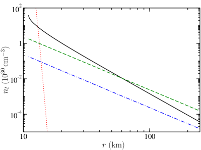
It turns out that addition of this exponential density profile near the neutrino sphere facilitates the multiangle simulations of neutrino flavor transformation. In Fig. 2 we plot the net electron number density

$$n_{e}=Y_{e}n_{\mathrm{b}}$$ (19)

obtained from the exponential profile in Eq. (17). For comparison, we also plot $n_{e}(r)$ obtained from the constant entropy profile [Eq. (16)] with entropy per baryon $S=140$ and 250. In both Fig. 2 and in the rest of the paper, we take $M_{\mathrm{NS}}=1.4\,M_{\odot}$, $R_{\nu}=11$ km, $Y_{e}=0.4$, $g_{\mathrm{s}}=11/2$, $n_{\mathrm{b}0}=1.63\times 10^{36}\,\mathrm{cm}^{-3}$ and $h_{\mathrm{NS}}=0.18\,\mathrm{km}$. Note that once we have specified $n_{\mathrm{b}0}$ and $h_{\mathrm{NS}}$ our model for the physical environment in the hot bubble is completely determined by the choice of entropy per baryon $S$. In units of Boltzmann constant per baryon, we expect $S\sim 100$ in the hot bubble Qian and Woosley (1996).

II.2 Neutrino Flavor Transformation in Supernovae

Our objective is to study the flavor evolution of the neutrino field when $\nu_{e}$ and $\bar{\nu}_{e}$ mix with neutrinos and antineutrinos of another active flavor (say $\nu_{\tau}$ and $\bar{\nu}_{\tau}$). We write the wave function of the flavor doublet of a neutrino (or antineutrino) as

$$\psi_{\nu}=\left(\begin{array}[]{c}a\\ b\end{array}\right),$$ (20)

where $a$ and $b$ are the amplitudes for a neutrino to be in the $\nu_{e}$ ($\bar{\nu}_{e}$) and $\nu_{\tau}$ ($\bar{\nu}_{\tau}$) flavor states, respectively. The flavor evolution of $\psi_{\nu_{\underline{\alpha}}}$ is determined by the Schrödinger equation (see, e.g., Ref. Qian and Fuller (1995a))

$$\mathrm{i}\frac{\mathrm{d}}{\mathrm{d}t}\psi_{\nu_{\underline{\alpha}}}=H\psi_{\nu_{\underline{\alpha}}}=\frac{1}{2}\left(\begin{array}[]{cc}-\Delta\cos 2\theta+A+B&\Delta\sin 2\theta+B_{e\tau}\\ \Delta\sin 2\theta+B_{e\tau}^{*}&\Delta\cos 2\theta-A-B\end{array}\right)\psi_{\nu_{\underline{\alpha}}},$$ (21)

where $\theta$ is the vacuum mixing angle, $\Delta$, $A$ and $B_{(e\tau)}$ are the potentials induced by neutrino mass difference, matter, and background neutrinos, respectively. One obtains the appropriate Hamiltonian for antineutrinos by making the transformation

$$A\longrightarrow-A,\qquad B\longrightarrow-B,\qquad B_{e\tau}\longrightarrow-B_{e\tau}^{*}.$$ (22)

The vacuum potential is defined as

$$\Delta\equiv\frac{\delta m^{2}}{2E_{\nu}},$$ (23)

where $\delta m^{2}$ is the neutrino mass-squared difference, and $E_{\nu}$ is the energy of the neutrino. (Note that we also use $q$ as the energy or the magnitude of the momentum of a neutrino in this section, which is the same as $E_{\nu}$.) We define the mass-squared difference in terms of the appropriate neutrino mass eigenvalues $m_{1}$ and $m_{3}$ to be $\delta m^{2}\equiv m_{3}^{2}-m_{1}^{2}$. In what follows we employ the normal ($\delta m^{2}=\delta m_{\mathrm{atm}}^{2}$) and inverted ($\delta m^{2}=-\delta m_{\mathrm{atm}}^{2}$) mass hierarchies. The matter potential is

$$A=\sqrt{2}G_{\mathrm{F}}n_{e}=\sqrt{2}G_{\mathrm{F}}Y_{e}n_{\mathrm{b}},$$ (24)

where $G_{\mathrm{F}}$ is the Fermi coupling constant. We define a reduced density matrix $\varrho_{\nu}$ (in the flavor basis) from $\psi_{\nu}$ as

$$\varrho_{\nu}\equiv\frac{1}{2}\left(\begin{array}[]{cc}|a|^{2}-|b|^{2}&2ab^{*}\\ 2a^{*}b&-|a|^{2}+|b|^{2}\end{array}\right).$$ (25)

Note that this definition applies for neutrinos and antineutrinos. This is, however, different from the convention adopted in Ref. Sigl and Raffelt (1993). Using Eq. (25), the neutrino-neutrino forward scattering part of the Hamiltonian in Eq. (21) can be written as

$$H_{\nu\nu} =\frac{1}{2}\left(\begin{array}[]{cc}B&B_{e\tau}\\ B_{e\tau}^{*}&-B\end{array}\right)$$ (26c)

$$=\sqrt{2}G_{\mathrm{F}}\sum_{\alpha}\Big{[}\int(1-{\bf\hat{q}}\cdot{\bf\hat{q}^{\prime}})\varrho_{\nu_{\underline{\alpha}}}({\bf q^{\prime}})\,\mathrm{d}n_{\nu_{\underline{\alpha}}}({\bf q^{\prime}})\mathrm{d}q^{\prime}-\int(1-{\bf\hat{q}}\cdot{\bf\hat{q}^{\prime}})\varrho_{\bar{\nu}_{\underline{\alpha}}}^{*}({\bf q^{\prime}})\,\mathrm{d}n_{\bar{\nu}_{\underline{\alpha}}}({\bf q^{\prime}})\mathrm{d}q^{\prime}\Big{]},$$ (26d)

where ${\bf q}$ and ${\bf q^{\prime}}$ are the momentum of the neutrino of interest and that of the background neutrino, respectively, and the flavor index is $\alpha=e$ or $\tau$. As mentioned above, neutrinos of the same initial flavor, energy and emission angle have identical flavor evolution. Consequently one must have

$$\varrho_{\nu}({\bf q})=\varrho_{\nu}(q,\vartheta).$$ (27)

We note that

$$\int{\bf\hat{q}}\cdot{\bf\hat{q}^{\prime}}F(\vartheta^{\prime})\,\mathrm{d}{\bf\hat{q}^{\prime}} =\int[\sin\vartheta\sin\vartheta^{\prime}(\sin\phi\sin\phi^{\prime}+\cos\phi\cos\phi^{\prime})+\cos\vartheta\cos\vartheta^{\prime}]F(\vartheta^{\prime})\,\mathrm{d}(\cos\vartheta^{\prime})\mathrm{d}\phi^{\prime}$$ (28a)

$$=2\pi\int\cos\vartheta\cos\vartheta^{\prime}F(\vartheta^{\prime})\,\mathrm{d}(\cos\vartheta^{\prime}),$$ (28b)

where $F(\vartheta)$ is an arbitrary function of $\vartheta$, and we have used the cylindrical symmetry around the $z$–axis in deriving Eq. (28b). Using Eqs. (5), (11) and (28), one can rewrite Eq. (26d) as

$$H_{\nu\nu}=\frac{\sqrt{2}G_{\mathrm{F}}}{2\pi R_{\nu}^{2}}\sum_{\alpha}\int(1-\cos\vartheta\cos\vartheta^{\prime})\left[\varrho_{\nu_{\underline{\alpha}}}(q^{\prime},\vartheta^{\prime})f_{\nu_{\underline{\alpha}}}(q^{\prime})\frac{L_{\nu_{\underline{\alpha}}}}{\langle E_{\nu_{\underline{\alpha}}}\rangle}-\varrho_{\bar{\nu}_{\underline{\alpha}}}^{*}(q^{\prime},\vartheta^{\prime})f_{\bar{\nu}_{\underline{\alpha}}}(q^{\prime})\frac{L_{\bar{\nu}_{\underline{\alpha}}}}{\langle E_{\bar{\nu}_{\underline{\alpha}}}\rangle}\right]\,\mathrm{d}(\cos\vartheta^{\prime})\mathrm{d}q^{\prime}.$$ (26d^′)

As noted in the introduction, previous simulations have used the single-angle approximation, wherein one assumes that the flavor evolution history of a neutrino is trajectory independent,

$$\varrho_{\nu}({\bf q})=\varrho_{\nu}(q),$$ (27^′)

and neutrinos on any trajectory transform in the same way as neutrinos propagating in the radial direction. Using the single-angle approximation, Eq. (26d^′) can be further simplified to

$$H_{\nu\nu}=\frac{\sqrt{2}G_{\mathrm{F}}}{2\pi R_{\nu}^{2}}D(r/R_{\nu})\sum_{\alpha}\int\left[\varrho_{\nu_{\underline{\alpha}}}(q^{\prime})f_{\nu_{\underline{\alpha}}}(q^{\prime})\frac{L_{\nu_{\underline{\alpha}}}}{\langle E_{\nu_{\underline{\alpha}}}\rangle}-\varrho_{\bar{\nu}_{\underline{\alpha}}}^{*}(q^{\prime})f_{\bar{\nu}_{\underline{\alpha}}}(q^{\prime})\frac{L_{\bar{\nu}_{\underline{\alpha}}}}{\langle E_{\bar{\nu}_{\underline{\alpha}}}\rangle}\right]\,\mathrm{d}q^{\prime},$$ (26d^′′)

where the geometric factor $D(r/R_{\nu})$ is defined as

$$D(r/R_{\nu})\equiv\frac{1}{2}\left[1-\sqrt{1-\left(\frac{R_{\nu}}{r}\right)^{2}}\right]^{2}.$$ (29)

Although our simulations are carried out by solving Eq. (21) numerically, the spin analogue of the wave function formalism (see, e.g., Ref. Duan et al. (2005)) provides an intuitive way of understanding the results of our simulations. The wave function of a neutrino $\psi_{\nu}$ in Eq. (20) can be mapped into a Neutrino Flavor Iso-Spin (NFIS) vector $\bm{\varsigma}$ using the Pauli matrices ${\bm{\sigma}}$:

$$\bm{\varsigma}_{\nu_{\underline{\alpha}}} \equiv\psi_{\nu_{\underline{\alpha}}}^{\dagger}\frac{\bm{\sigma}}{2}\psi_{\nu_{\underline{\alpha}}}=\frac{1}{2}\left(\begin{array}[]{c}2\mathrm{Re}(a^{*}b)\\ 2\mathrm{Im}(a^{*}b)\\ |a|^{2}-|b|^{2}\end{array}\right);$$ (30d)

$$\bm{\varsigma}_{\bar{\nu}_{\underline{\alpha}}} \equiv(\sigma_{y}\psi_{\bar{\nu}_{\underline{\alpha}}})^{\dagger}\frac{\bm{\sigma}}{2}(\sigma_{y}\psi_{\bar{\nu}_{\underline{\alpha}}})=-\frac{1}{2}\left(\begin{array}[]{c}2\mathrm{Re}(ab^{*})\\ 2\mathrm{Im}(ab^{*})\\ |a|^{2}-|b|^{2}\end{array}\right).$$ (30h)

Note that the extra $\sigma_{y}$ in Eq. (30h) transforms $\overline{\bf 2}$ of SU(2), the fundamental representation of antiparticles, into ${\bf 2}$, the fundamental representation of particles. As a result, $\bm{\varsigma}_{\bar{\nu}_{\underline{\alpha}}}$ transforms in the same way as $\bm{\varsigma}_{\nu_{\underline{\alpha}}}$ under rotations. We also note the NFIS’s $\bm{\varsigma}_{\nu}$ defined in Eq. (30) have constant magnitude 1/2. For a neutrino $\nu_{\underline{\alpha}}$, $\varsigma_{\nu_{\underline{\alpha}}z}=+1/2$ ($-1/2$) for the pure $\nu_{e}$ ($\nu_{\tau}$) state, where $\varsigma_{\nu_{\underline{\alpha}}z}$ is the third component of the NFIS. For an antineutrino $\bar{\nu}_{\underline{\alpha}}$, $\varsigma_{\bar{\nu}_{\underline{\alpha}}z}=+1/2$ ($-1/2$) for the pure $\bar{\nu}_{\tau}$ ($\bar{\nu}_{e}$) state.

The NFIS $\bm{\varsigma}_{\nu}(q,\vartheta)$ for either a neutrino or an antineutrino obeys the equation of motion

$$\begin{split}\frac{\mathrm{d}}{\mathrm{d}t}\bm{\varsigma}_{\nu}(q,\vartheta)&=\bm{\varsigma}_{\nu}(q,\vartheta)\times\Big{[}\mathbf{H}^{\mathrm{eff}}(q)\\ &\quad+\frac{1}{2\pi R_{\nu}^{2}}\sum_{\nu^{\prime}}\int\mu(\vartheta,\vartheta^{\prime})\bm{\varsigma}_{\nu^{\prime}}(q^{\prime},\vartheta^{\prime})\\ &\quad\times f_{\nu^{\prime}}(q^{\prime})\frac{L_{\nu^{\prime}}}{\langle E_{\nu^{\prime}}\rangle}\,\mathrm{d}(\cos\vartheta^{\prime})\mathrm{d}q^{\prime}\Big{]},\end{split}$$ (31)

where $q$ and $\vartheta$ are the magnitude and polar angle of the momentum of the neutrino, $\mathbf{H}^{\mathrm{eff}}$ is an effective field, and $\mu(\vartheta,\vartheta^{\prime})$ is the coupling coefficient between $\bm{\varsigma}_{\nu}(q,\vartheta)$ and the background neutrino $\bm{\varsigma}_{\nu^{\prime}}(q^{\prime},\vartheta^{\prime})$ with

$$\mu(\vartheta,\vartheta^{\prime})\equiv-2\sqrt{2}G_{\mathrm{F}}(1-\cos\vartheta\cos\vartheta^{\prime}).$$ (32)

The summation index $\nu^{\prime}$ in Eq. (31) runs over $\nu_{\underline{e}}$, $\nu_{\underline{\tau}}$, $\bar{\nu}_{\underline{e}}$, and $\bar{\nu}_{\underline{\tau}}$. According to Eq. (31), the motion of a NFIS in flavor space is analogous to that of a magnetic spin which simultaneously precesses around a “magnetic field” $\mathbf{H}^{\mathrm{eff}}$ and the other “spins”. The “magnetic field” $\mathbf{H}^{\mathrm{eff}}$ is composed of two components in our case,

$$\mathbf{H}^{\mathrm{eff}}(q)=\mu_{\mathrm{V}}(q)\mathbf{H}_{\mathrm{V}}+\mu_{e}\mathbf{H}_{e}.$$ (33)

In Eq. (33) $\mathbf{H}_{\mathrm{V}}$ stems from neutrino mass difference and can be written as

$$\mathbf{H}_{\mathrm{V}}\equiv-{\bf\hat{e}}^{\mathrm{f}}_{x}\sin 2\theta+{\bf\hat{e}}^{\mathrm{f}}_{z}\cos 2\theta,$$ (34)

where ${\bf\hat{e}}^{\mathrm{f}}_{x(y,z)}$ are the orthogonal unit vectors in flavor space corresponding to $\sigma_{x(y,z)}$. Here we define

$$\mu_{\mathrm{V}}(q)\equiv\pm\frac{\delta m^{2}}{2q},$$ (35)

where the plus sign is for neutrinos and the minus sign is for antineutrinos. With these definitions, neutrinos possess positive (negative) “magnetic moments” $\mu_{\mathrm{V}}$ and antineutrinos possess negative (positive) ones if $\delta m^{2}>0$ ($\delta m^{2}<0$). Because neutrinos can have different energies, $\mu_{\mathrm{V}}$ varies from $-\infty$ to $+\infty$. The second term in Eq. (33) is induced by matter (neutrino-electron forward scattering), and we can write

$$\mathbf{H}_{e} \equiv-{\bf\hat{e}}^{\mathrm{f}}_{z}n_{\mathrm{b}}Y_{e}$$ (36)

and

$$\mu_{e} \equiv\sqrt{2}G_{\mathrm{F}}.$$ (37)

Before we show the results of our simulations, we shall estimate the “MSW resonance radius” $r_{\mathrm{MSW}}$ for a neutrino with a typical energy. The MSW resonance condition would be

$$\Delta\cos 2\theta=A(r_{\mathrm{MSW}})$$ (38)

if we ignore the neutrino-neutrino flavor-diagonal potential $B$. We will take $|\delta m^{2}|=3\times 10^{-3}\,\mathrm{eV}^{2}$, the atmospheric value, and we will take the effective $2\times 2$ vacuum mixing angle to be $\theta=0.1$. Note that this value is well below the experimental limit on $\theta_{13}$. For these parameters, the MSW resonance radius of a neutrino in the case of normal mass hierarchy ($\delta m^{2}>0$) or an antineutrino in the case of inverted mass hierarchy ($\delta m^{2}<0$) with energy $E_{\nu}=10$ MeV is $r_{\mathrm{MSW}}\simeq 127$ and 59 km for $S=140$ and 250, respectively. We shall also estimate the radius for significant neutrino flavor transformation if neutrinos and antineutrinos are in the “synchronization” mode Pastor et al. (2002). When neutrinos are in the synchronization mode, all the NFIS’s behave as one “magnetic spin” with

$$\pm\frac{\delta m^{2}}{2E_{\mathrm{sync}}}\equiv\langle\mu_{\mathrm{V}}\rangle=\frac{\displaystyle\sum_{\nu}\frac{L_{\nu}}{\langle E_{\nu}\rangle}\int\mu_{\mathrm{V}}(q)\varsigma_{\nu z}f_{\nu}(q)\,\mathrm{d}q}{\displaystyle\sum_{\nu}\frac{L_{\nu}}{\langle E_{\nu}\rangle}\int\varsigma_{\nu z}f_{\nu}(q)\,\mathrm{d}q},$$ (39)

where we have assumed all the NFIS’s are aligned or antialigned with ${\bf\hat{e}}^{\mathrm{f}}_{z}$. Because $E_{\mathrm{sync}}$ is positive, the sign of the first term (left hand side) of Eq. (39) should be chosen to be the same as that of the product $\delta m^{2}\langle\mu_{\mathrm{V}}\rangle$. If $\langle\mu_{\mathrm{V}}\rangle>0$ and $\delta m^{2}>0$, all the neutrinos and antineutrinos go through the same conversion process as a neutrino of energy $E_{\mathrm{sync}}$ at $r_{\mathrm{MSW}}(E_{\mathrm{sync}})$. Similarly, if $\langle\mu_{\mathrm{V}}\rangle>0$ and $\delta m^{2}<0$, all the neutrinos and antineutrinos go through the same conversion process as an antineutrino of energy $E_{\mathrm{sync}}$ at $r_{\mathrm{MSW}}(E_{\mathrm{sync}})$. Neutrino flavor transformation is suppressed for other synchronization scenarios. For the parameters we have chosen, we find that $\langle\mu_{\mathrm{V}}\rangle>0$ if $\delta m^{2}>0$, and $\langle\mu_{\mathrm{V}}\rangle<0$ if $\delta m^{2}<0$. The characteristic energy of the synchronization mode is $E_{\mathrm{sync}}\simeq 2.47$ MeV for both cases. Therefore, in the synchronized mode neutrinos and antineutrinos should transform simultaneously at $r_{\mathrm{MSW}}(E_{\mathrm{sync}})\simeq 80$ and 37 km for $S=140$ and 250, respectively, if $\delta m^{2}>0$. These neutrinos/antineutrinos would experience very little flavor conversion if $\delta m^{2}<0$.

A special case of synchronized behavior is the Background Dominant Solution (BDS) Fuller and Qian (2006) where the NFIS’s rotate in the plane spanned by ${\bf\hat{e}}^{\mathrm{f}}_{x}$ and ${\bf\hat{e}}^{\mathrm{f}}_{y}$ in flavor space. One of the necessary conditions for the BDS with large-scale simultaneous neutrino and antineutrino flavor transformation is that the flavor off-diagonal neutrino background potential $B_{e\tau}$ dominates. To see this condition more clearly, we define the effective net $\nu_{\underline{e}}$ number density along the radial trajectory as

$$n_{\nu_{\underline{e}}}^{\mathrm{eff}} =\int(1-{\bf\hat{z}}\cdot{\bf\hat{q}^{\prime}})\,\mathrm{d}n_{\nu_{\underline{e}}}({\bf q^{\prime}})\mathrm{d}q^{\prime}-\int(1-{\bf\hat{z}}\cdot{\bf\hat{q}^{\prime}})\,\mathrm{d}n_{\bar{\nu}_{\underline{e}}}({\bf q^{\prime}})\mathrm{d}q^{\prime}$$ (40a)

$$=\frac{D(r/R_{\nu})}{2\pi R_{\nu}^{2}}\left(\frac{L_{\nu_{\underline{e}}}}{\langle E_{\nu_{\underline{e}}}\rangle}-\frac{L_{\bar{\nu}_{\underline{e}}}}{\langle E_{\bar{\nu}_{\underline{e}}}\rangle}\right)$$ (40b)

$$=(1.66\times 10^{32}\,\mathrm{cm}^{-3})\left[1-\sqrt{1-\left(\frac{R_{\nu}}{r}\right)^{2}}\right]^{2}\left(\frac{10\,\mathrm{km}}{R_{\nu}}\right)^{2}\left[\frac{L_{\nu_{\underline{e}}}/(10^{51}\,\mathrm{erg/s})}{\langle E_{\nu_{\underline{e}}}\rangle/(10\,\mathrm{MeV})}-\frac{L_{\bar{\nu}_{\underline{e}}}/(10^{51}\,\mathrm{erg/s})}{\langle E_{\bar{\nu}_{\underline{e}}}\rangle/(10\,\mathrm{MeV})}\right].$$ (40c)

Note that $|B_{e\tau}|=\sqrt{2}G_{\mathrm{F}}|n_{\nu_{\underline{e}}}^{\mathrm{eff}}|$ and $B=0$ if the BDS obtains. (Obviously, if no flavor transformation has occurred, $B_{e\tau}=0$ and $B=\sqrt{2}G_{\mathrm{F}}n_{\nu_{\underline{e}}}^{\mathrm{eff}}$.) We plot $n_{\nu_{\underline{e}}}^{\mathrm{eff}}(r)$ together with $n_{e}(r)$ used in our simulations in Fig. 2. The neutrino background potential will dominate the matter potential on the radial trajectory if $n_{\nu_{\underline{e}}}^{\mathrm{eff}}>n_{e}$, which corresponds to a radius as low as $r\sim 13$ km for the parameters we have chosen.

For numerical simplicity, we have fixed $Y_{e}=0.4$ in our simulations. Of course, the value of $Y_{e}$ actually varies with the radius and is affected by $\nu_{e}$ and $\bar{\nu}_{e}$ fluxes through the weak interactions Fuller et al. (1992); Qian et al. (1993)

$$\nu_{e}+n \rightleftharpoons p+e^{-},$$ (41a)

$$\bar{\nu}_{e}+p \rightleftharpoons n+e^{+}.$$ (41b)

The rates of these processes can also be affected by weak magnetism corrections Horowitz and Li (1999); Horowitz (2002). In the numerical simulations presented below we have not included neutrino/antineutrino flavor transformation feedback through these processes on $Y_{e}$. This is an important aspect of the physics of the supernova environment which we leave to a subsequent paper.

Models for r-process nucleosynthesis can be sensitive to the value of $Y_{e}$ in the region where $T\gtrsim 0.1$ MeV Qian et al. (1993); Qian and Fuller (1995a). For our chosen density profile, $T=0.1$ MeV occurs at $r\sim 139$ and 78 km for entropy per baryon $S=140$ and 250, respectively. These values of radius are well outside our simple estimates for where conventional MSW, synchronization, or BDS-like flavor conversion could occur. The numerical results to be discussed in the next section will give us a much better idea of where large-scale neutrino flavor transformation actually occurs.

III Multiangle Numerical Simulations

In Sec. III.1 we discuss our numerical calculations, and point out two potential pitfalls in any multiangle simulation. In Sec. III.2 we show the main results from our multiangle simulations. For the simulation results presented in this section we have taken $|\delta m^{2}|=3\times 10^{-3}\,\mathrm{eV}^{2}$, $\theta=0.1$, $L_{\nu_{\underline{e}}}=L_{\bar{\nu}_{\underline{e}}}=L_{\nu_{\underline{\tau}}}=L_{\bar{\nu}_{\underline{\tau}}}=10^{51}$ erg/s and $S=140$ unless otherwise stated.

III.1 Numerical Scheme

We have developed two independent sets of numerical codes using different computer languages. We have used them to provide cross checks to obtain consistent results. Both codes employ a large multidimensional array of neutrino wave functions $\psi_{\nu_{\underline{\alpha}}}(E_{\nu},\cos\vartheta_{0})$ and $\psi_{\bar{\nu}_{\underline{\alpha}}}(E_{\nu},\cos\vartheta_{0})$ and evolve them simultaneously following the scheme outlined in Sec. II. Each code employs an adaptive step size control mechanism, but the two codes have different ways of estimating errors and adjusting step sizes. The energy bins are chosen to have equal sizes for convenience in comparing neutrino energy spectra at different radii. The angle bins are determined in such a way that each bin has the same size in $\cos\vartheta$ at radius $R_{\mathrm{bin}}$. In most cases we have taken $R_{\mathrm{bin}}=R_{\nu}$, the neutrino sphere radius. Note that the angle bins have different sizes in $\cos\vartheta$ if $r\neq R_{\mathrm{bin}}$.

At the basic level, both codes obtain $\psi_{\nu}(l+\delta l)$ from $\psi_{\nu}(l)$ by using the following equation as a first step:

$$\psi_{\nu}(l+\delta l) \simeq\exp(-\mathrm{i}H\delta l)\psi_{\nu}(l)$$ (42a)

$$=\frac{1}{\lambda}\begin{pmatrix}\lambda\cos(\lambda\delta l)-\mathrm{i}h_{11}\sin(\lambda\delta l)&-\mathrm{i}h_{12}\sin(\lambda\delta l)\\ -\mathrm{i}h_{12}^{*}\sin(\lambda\delta l)&\lambda\cos(\lambda\delta l)+\mathrm{i}h_{11}\sin(\lambda\delta l)\end{pmatrix}\psi_{\nu}(l),$$ (42b)

where $h_{11}$ and $h_{12}$ are the diagonal and off-diagonal elements of the Hamiltonian $H$, and

$$\lambda\equiv\sqrt{h_{11}^{2}+|h_{12}|^{2}}.$$ (43)

[Although not written out explicitly, the Hamiltonian $H$ and its elements in the above equations have dependence on both the Affine parameter $l$ and trajectory angle $\vartheta$, as can be inferred from Eqs. (21) through (26d^′).] We note that Eq. (42) preserves the unitarity of $\psi_{\nu}$ automatically. We also note that Eq. (42) becomes exact if $H$ is independent of spatial coordinate. Therefore, the step sizes employed in our numerical codes are not restricted by the size of $H$ but are restricted by the rate of change of $H$.

In the course of our work we have discovered two pitfalls which apply to any multiangle scheme. Failure to avoid these pitfalls may lead to quantitatively or qualitatively inaccurate results (see Fig. 3).

Figure 3: (Color online) Average $\nu_{e}$ survival probability $\langle P_{\nu_{\underline{e}}\nu_{e}}(r)\rangle$ along the radial trajectory ($\cos\vartheta_{0}$=1) with the normal mass hierarchy in different numerical schemes. Here the average is done over the initial energy spectra of $\nu_{\underline{e}}$. The dot-dashed line uses 160 angle bins and error tolerance $10^{-5}$ in each step without the initial baryon density profile $n_{\mathrm{b}}^{\prime}$. The dashed and solid lines both include $n_{\mathrm{b}}^{\prime}$ and employ error tolerance $10^{-10}$, but use 256 and 512 angle bins, respectively. Calculations with 768, 1024 and 1407 angle bins in different binning schemes produce curves which fall on the solid line.

The first potential problem has to do with the exponential term $n_{\mathrm{b}}^{\prime}$ in the profile for the baryon density [see Eq. (17)]. The baryon density is very high near the neutrino sphere when $n_{\mathrm{b}}^{\prime}$ is included. This sometimes forces numerical schemes to employ initially very small step sizes. The numerical codes using the single-angle approximation can generally drop $n_{\mathrm{b}}^{\prime}$ without loss of accuracy at large radius. These codes will of course run faster without $n_{\mathrm{b}}^{\prime}$. However, in multiangle simulations, ignoring $n_{\mathrm{b}}^{\prime}$ makes the background neutrino potential $B$ much bigger than the matter potential $A$ even at the neutrino sphere. As a result, the evolution histories of neutrino flavors on all trajectories are strongly coupled starting from the beginning. This strong correlation among all trajectories also forces small step sizes. In addition, without $n_{\mathrm{b}}^{\prime}$ there is a tendency for neutrinos to undergo flavor transformation very close to the neutrino sphere. This behavior is suppressed if there is a large and dominant matter potential $A$. Including $n_{\mathrm{b}}^{\prime}$ makes the matter potential $A(R_{\nu})$ much bigger and this helps keep neutrinos in their initial flavor states, at least for the significant range of neutrino/antineutrino energies and for our chosen value of $|\delta m^{2}|\simeq\delta m^{2}_{\mathrm{atm}}$. We also note that neutrinos on different trajectories propagate through different distances. A big matter potential breaks the correlation between neutrinos on different trajectories and lets them evolve independently for awhile.

These considerations can be cast in simpler, more physical terms. In the relatively narrow region near the neutrino sphere where $n_{\mathrm{b}}^{\prime}$ dominates it has the effect of changing, or “resetting”, the neutrino wavefunctions relative to what they would have been had we employed the unphysical low-density profile all the way to the neutrino sphere. In the latter unphysical case, neutrinos are in flavor eigen states at the neutrino sphere, and the NFIS’s are perfectly aligned with each other yet slightly deviated from the total effective field $\mathbf{H}^{\mathrm{eff}}$. The effects of this unphysical setup does not go away quickly with increasing radius because the coupling among the NFIS’s (arising from neutrino-neutrino forward scatterings) is so strong. If the exponential baryon density profile $n_{\mathrm{b}}^{\prime}$ is added, the overwhelming matter field $\mathbf{H}_{e}$ at the neutrino sphere not only makes the NFIS’s more aligned with $\mathbf{H}^{\mathrm{eff}}$, but also breaks the coupling of the NFIS’s propagating along different trajectories. In the short distance where the matter field $\mathbf{H}_{e}$ dominates, the NFIS’s on different trajectories have traveled different distances and so have developed different phases. At the radius where $n_{\mathrm{b}}^{\prime}$ becomes negligible, the NFIS’s are effectively “reset” to a more physical condition than one would obtain without $n_{\mathrm{b}}^{\prime}$.

The other pitfall is that one may use an insufficient number of angle bins. Assuming that there has been very little neutrino flavor conversion close to the neutrino sphere where $r\sim R_{\nu}$, we can write

$$B(r,\vartheta) \simeq\frac{\sqrt{2}G_{\mathrm{F}}}{2\pi R_{\nu}^{2}}\left(\frac{L_{\nu_{\underline{e}}}}{\langle E_{\nu_{\underline{e}}}\rangle}-\frac{L_{\bar{\nu}_{\underline{e}}}}{\langle E_{\bar{\nu}_{\underline{e}}}\rangle}\right)\left[1-\sqrt{1-\left(\frac{R_{\nu}}{r}\right)^{2}}-\frac{1}{2}\cos\vartheta\left(\frac{R_{\nu}}{r}\right)^{2}\right],$$ (44a)

$$B_{e\tau}(r,\vartheta) \simeq 0.$$ (44b)

For a small step size $\delta l$, one has

$$\psi_{\nu_{\underline{\alpha}}}(l+\delta l) \simeq\exp(-\mathrm{i}H\delta l)\psi_{\nu_{\underline{\alpha}}}(l)$$ (45a)

$$\simeq\begin{pmatrix}e^{-\mathrm{i}(A+B)\delta l}&-\mathrm{i}\frac{\displaystyle\Delta\sin 2\theta}{\displaystyle A+B}\sin[(A+B)\delta l]\\ -\mathrm{i}\frac{\displaystyle\Delta\sin 2\theta}{\displaystyle A+B}\sin[(A+B)\delta l]&e^{\mathrm{i}(A+B)\delta l}\end{pmatrix}\psi_{\nu_{\underline{\alpha}}}(l),$$ (45b)

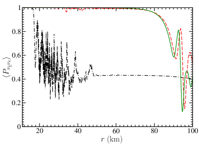
where we have used the fact that $A+B\gg\Delta$ at $r\sim R_{\nu}$. It is the off-diagonal elements of the transformation matrix in Eq. (45b) that govern the exchange of the two flavor components of a neutrino wave function. These off-diagonal terms, we note, are oscillatory functions of the $B$ potential and the step size $\delta l$, both of which have angular dependence [see Eqs. (2) and (44a)]. Physically, this oscillatory feature with respect to angles is suppressed by strong correlation among neutrinos on different trajectories. Numerical codes without enough angular resolution, however, could allow a spurious “cross-talk” between angle zones which artificially strengthens flavor oscillations. This unphysical feedback could produce substantial neutrino flavor conversion even at low radius in some numerical schemes.

$\begin{array}[]{@{}c@{\hspace{\myfigsep}}c@{}}\includegraphics*[width=208.13574pt,keepaspectratio]{fig4a.eps}\hfil\hskip 17.34189pt&\includegraphics*[width=208.13574pt,keepaspectratio]{fig4b.eps}\\ \includegraphics*[width=208.13574pt,keepaspectratio]{fig4c.eps}\hfil\hskip 17.34189pt&\includegraphics*[width=208.13574pt,keepaspectratio]{fig4d.eps}\end{array}$

Figure 4: (Color online) Plots of average survival probability $\langle P_{\nu_{\underline{e}}\nu_{e}}\rangle$ (left panels) and $\langle P_{\bar{\nu}_{\underline{e}}\bar{\nu}_{e}}\rangle$ (right panels) with the normal (upper panels) and inverted (lower panels) neutrino mass hierarchies, respectively. The solid and dotted lines give average survival probabilities along trajectories with $\cos\vartheta_{0}=1$ and $\cos\vartheta_{0}=0$, respectively, as computed in the multiangle simulations. The dot-dashed lines and the dashed lines characterize the limits where neutrinos and antineutrino undergo flavor transformation individually ($L_{\nu}=0$ and $A$ potential only) and simultaneously (full synchronization), respectively. The dashed line is not distinguishable from the dot-dashed line in panel (c).

In Fig. 3 we plot average survival probability $\langle P_{\nu_{\underline{e}}\nu_{e}}(r)\rangle$ along the radial trajectory with the normal mass hierarchy using different numerical schemes (error tolerance, number of angle bins, etc.). Here $P_{\nu_{\underline{e}}\nu_{e}}(r)$ is the probability for a $\nu_{\underline{e}}$ to be a $\nu_{e}$ at radius $r$, and the average is done over the initial energy distribution for $\nu_{\underline{e}}$. (As mentioned above, we use $\nu_{\underline{\alpha}}$ and $\bar{\nu}_{\underline{\alpha}}$ to denote the neutrinos and antineutrinos that are emitted in flavor state $\alpha$ at the neutrino sphere.) One sees that spurious neutrino flavor transformation (dot-dashed line) could occur at low radius with a combination of insufficient number of angle bins, a loose error control, and neglect of $n_{\mathrm{b}}^{\prime}$. If we employ $L_{\nu}=10^{51}$ erg/s and choose a stringent error tolerance ($\sim 10^{-10}$) at each step, we find that it takes $\gtrsim 500$ angle bins in order to achieve convergence and run-to-run consistency. Because the $B$ potential increases with neutrino luminosity, we expect that even more angle bins would be required to obtain convergence at larger neutrino luminosity.

Our numerical simulations generally employ $\gtrsim 500$ angle bins and $\gtrsim 500$ energy bins for each neutrino species. Typically, our codes execute $\gtrsim 10^{5}$ steps during each production run. It is clear that multiangle simulations are only feasible using large-scale parallel computation.

III.2 Simulation Results

$\begin{array}[]{@{}c@{\hspace{\myfigsep}}c@{}}\includegraphics*[width=208.13574pt,keepaspectratio]{fig5a.eps}\hfil\hskip 17.34189pt&\includegraphics*[width=208.13574pt,keepaspectratio]{fig5b.eps}\end{array}$

Figure 5: (Color online) Plots of $P_{\nu_{\underline{e}}\nu_{e}}(r)$ with the normal mass hierarchy. Panel (a) is for the radial trajectory ($\cos\vartheta_{0}=1$), and (b) is for the tangential trajectory ($\cos\vartheta_{0}=0$). The dot-dashed, dotted, dashed and solid lines are for $\nu_{\underline{e}}$ of energies 6.95, 8.95, 10.95 and 14.95 MeV, respectively.

$\begin{array}[]{@{}c@{\hspace{\myfigsep}}c@{}}\includegraphics*[width=208.13574pt,keepaspectratio]{fig6a.eps}\hfil\hskip 17.34189pt&\includegraphics*[width=208.13574pt,keepaspectratio]{fig6b.eps}\\ \includegraphics*[width=208.13574pt,keepaspectratio]{fig6c.eps}\hfil\hskip 17.34189pt&\includegraphics*[width=208.13574pt,keepaspectratio]{fig6d.eps}\end{array}$

Figure 6: (Color online) Plots of $P_{\nu_{\underline{e}}\nu_{e}}(\cos\vartheta_{0})$ (left panels) and $P_{\bar{\nu}_{\underline{e}}\bar{\nu}_{e}}(\cos\vartheta_{0})$ (right panels) at $r\simeq 92.85$ km for the normal mass hierarchy (upper panels) and at $r\simeq 88.57$ km for the inverted mass hierarchy (lower panels). The dot-dashed, dotted, dashed and solid lines are for $\nu_{\underline{e}}$ or $\bar{\nu}_{\underline{e}}$ of energies 6.95, 8.95, 10.95 and 14.95 MeV, respectively.

In Fig. 4(a), we plot $\langle P_{\nu_{\underline{e}}\nu_{e}}(r)\rangle$ with the normal neutrino mass hierarchy ($\delta m^{2}>0$) on both the radial ($\cos\vartheta_{0}=1$) and tangential ($\cos\vartheta_{0}=0$) trajectories. For comparison, we also plot $\langle P_{\nu_{\underline{e}}\nu_{e}}(r)\rangle$ for the $L_{\nu}=0$ ($A$ potential only) case, which is obtained from the single-angle simulation by setting $L_{\nu}=0$. The $L_{\nu}=0$ case corresponds to the limit where neutrinos go through MSW resonances independently of each other. In the full synchronization limit, all neutrinos and antineutrinos undergo flavor transformation in the same way as does a $\nu_{\underline{e}}$ with energy $E_{\mathrm{sync}}$ in the standard MSW mechanism. Using only the matter potential, we have calculated $P_{\nu_{\underline{e}}\nu_{e}}$ for a $\nu_{\underline{e}}$ with energy $E_{\mathrm{sync}}$ propagating along the radial trajectory. The result is shown in Fig. 4(a). The results of our simulations are clearly different from those in the $L_{\nu}=0$ and full synchronization limits. In particular, our simulation has $\langle P_{\nu_{\underline{e}}\nu_{e}}(r)\rangle$ crossing the 1/2 line later than in the synchronization case, but earlier than in the $L_{\nu}=0$ case. We also note that $\langle P_{\nu_{\underline{e}}\nu_{e}}(r)\rangle$ oscillates and even bounces back after an initial decrease.

$\begin{array}[]{@{}c@{\hspace{\myfigsep}}c@{}}\includegraphics*[width=208.13574pt,keepaspectratio]{fig7a.eps}\hfil\hskip 17.34189pt&\includegraphics*[width=208.13574pt,keepaspectratio]{fig7b.eps}\\ \includegraphics*[width=208.13574pt,keepaspectratio]{fig7c.eps}\hfil\hskip 17.34189pt&\includegraphics*[width=208.13574pt,keepaspectratio]{fig7d.eps}\end{array}$

Figure 7: (Color online) Change of energy spectra of neutrinos (left panels) and antineutrinos (right panels) with the normal (upper panels) and inverted (lower panels) neutrino mass hierarchies. The dotted and dot-dashed lines are the spectra of neutrinos (antineutrinos) in the electron and tau flavors, respectively, at $r=R_{\nu}$, and the solid and dashed lines are the corresponding spectra at $r=250$ km.

In Fig. 4(b) we plot $\langle P_{\bar{\nu}_{\underline{e}}\bar{\nu}_{e}}(r)\rangle$ in the normal neutrino mass hierarchy scenario. The conventional MSW conversion of $\bar{\nu}_{e}$ is suppressed if $\delta m^{2}>0$, which is illustrated dramatically by the $L_{\nu}=0$ case. In the case of full synchronization, $\bar{\nu}_{e}$ will be converted into $\bar{\nu}_{\tau}$ in exactly the same way as $\nu_{e}$ is converted into $\nu_{\tau}$. The results of our simulations are again like neither of these limits. Unlike the $L_{\nu}=0$ case, the actual values of $\langle P_{\bar{\nu}_{\underline{e}}\bar{\nu}_{e}}(r)\rangle$ may substantially decrease at some values of radius, and unlike the full synchronization case, $\langle P_{\bar{\nu}_{\underline{e}}\bar{\nu}_{e}}(r)\rangle$ oscillates and bounces back to nearly unity at large radius.

The results of the inverted neutrino mass hierarchy ($\delta m^{2}<0$) are more surprising. These are plotted in panels (c) and (d) of Fig. 4. The full synchronization limit predicts no flavor conversion for both $\nu_{e}$ and $\bar{\nu}_{e}$, and the $L_{\nu}=0$ limit predicts that only antineutrinos will be converted. Our simulation finds substantial conversion of both $\nu_{e}$ and $\bar{\nu}_{e}$. Furthermore, this phenomenon occurs at a radius even smaller than that expected in the full synchronization limit with $\delta m^{2}>0$. Again, we note that in the inverted mass hierarchy scenario both $\langle P_{\nu_{\underline{e}}\nu_{e}}(r)\rangle$ and $\langle P_{\bar{\nu}_{\underline{e}}\bar{\nu}_{e}}(r)\rangle$ oscillate after flavor transformation starts.

In Fig. 5 we plot $P_{\nu_{\underline{e}}\nu_{e}}(r)$ for $\nu_{\underline{e}}$ with a few characteristic energies on both the radial and tangential trajectories. We have employed the normal mass hierarchy in this calculation. One sees that the $P_{\nu_{\underline{e}}\nu_{e}}(r)$ curves have similar trends with radius over most of the $\nu_{\underline{e}}$ energy range considered. This is especially true for the values of radius where neutrino flavor transformation has just become significant and for the tangential trajectory.

The results presented in Fig. 5 lead us to conclude that the flavor transformation histories of neutrinos on different trajectories can be very different. To illustrate this point more clearly, we plot in Fig. 6(a) $P_{\nu_{\underline{e}}\nu_{e}}(\cos\vartheta_{0})$ at $r\simeq 92.85\,\mathrm{km}$ for $\nu_{\underline{e}}$ with specified energies, and employing the normal mass hierarchy. Indeed the values of $P_{\nu_{\underline{e}}\nu_{e}}(\cos\vartheta_{0})$ vary with angle, especially around $\cos\vartheta_{0}=1$. Moreover, the trend of $P_{\nu_{\underline{e}}\nu_{e}}(\cos\vartheta_{0})$ with angle is similar for $\nu_{\underline{e}}$ with different energies over most of the energy range considered. This again demonstrates the collective feature of the neutrino flavor transformation in the hot bubble.

In Fig. 6(b) we plot the corresponding antineutrino survival probability $P_{\bar{\nu}_{\underline{e}}\bar{\nu}_{e}}(\cos\vartheta_{0})$. This also shows angular dependence and collective flavor transformation. In Fig. 6(c–d), we plot $P_{\nu_{\underline{e}}\nu_{e}}(\cos\vartheta_{0})$ and $P_{\bar{\nu}_{\underline{e}}\bar{\nu}_{e}}(\cos\vartheta_{0})$ with the same parameters as in panels (a–b) but at $r\simeq 88.57$ km and with the inverted mass hierarchy. It is interesting to see that, in addition to the features pointed out for panels (a–b), in the inverted mass hierarchy case both $P_{\nu_{\underline{e}}\nu_{e}}(\cos\vartheta_{0})$ and $P_{\bar{\nu}_{\underline{e}}\bar{\nu}_{e}}(\cos\vartheta_{0})$ oscillate over most of the range of $\cos\vartheta_{0}$.

In these simulations, significant neutrino flavor transformation ends at $r\sim 230$ km (Fig. 4). To see how the energy spectra of neutrinos and antineutrinos have been altered by flavor transformation, in Fig. 7(a) we plot both $\tilde{f}_{\nu_{\underline{e}}}(E)$ and $\tilde{f}_{\nu_{\underline{\tau}}}(E)$ at the neutrino sphere, and $\tilde{f}_{\nu_{e}}(E)$ and $\tilde{f}_{\nu_{\tau}}(E)$ at $r=250$ km. Here we have employed the normal mass hierarchy and we take $\tilde{f}_{\nu}(E)$ to be proportional to both $f_{\nu}(E)$ and the flux of $\nu$ [e.g., $\tilde{f}_{\nu_{e}}(E)\propto f_{\nu_{e}}(E)\sum_{\alpha}\int P_{\nu_{\underline{\alpha}}\nu_{e}}\mathrm{d}n_{\nu_{\underline{\alpha}}}$ and $\tilde{f}_{\nu_{\underline{e}}}(E)\propto f_{\nu_{\underline{e}}}(E)L_{\nu_{\underline{e}}}/\langle E_{\nu_{\underline{e}}}\rangle$], such that

$$1 =\sum_{\alpha}\int[\tilde{f}_{\nu_{\alpha}}(E)+\tilde{f}_{\bar{\nu}_{\alpha}}(E)]\,\mathrm{d}E$$ (46a)

$$=\sum_{\alpha}\int[\tilde{f}_{\nu_{\underline{\alpha}}}(E)+\tilde{f}_{\bar{\nu}_{\underline{\alpha}}}(E)]\,\mathrm{d}E.$$ (46b)

Here the scheme for angle-averaging the energy spectra is simply the angle dependence in the neutrino flux “seen” by a nucleon at radius $r$. As a result, the angle-averaged spectra shown are those appropriate for use in the weak interaction rates. It is interesting to see that most of the low-energy ($E_{\nu}\lesssim 9.5$ MeV) $\nu_{e}$ are converted into $\nu_{\tau}$, while a significant fraction of high energy $\nu_{e}$ survive. We also plot the corresponding energy spectra of $\bar{\nu}_{e}$ and $\bar{\nu}_{\tau}$ in Fig. 7(b). The energy spectra of antineutrinos are changed very little in the normal mass hierarchy scenario. The energy spectra of neutrinos and antineutrinos in the inverted mass hierarchy scenario are plotted in Fig. 7(c) and (d), respectively. In these figures, both $\nu_{e}$ and $\bar{\nu}_{e}$ swap spectra with $\nu_{\tau}$ and $\bar{\nu}_{\tau}$, respectively, over a significant energy range.

The numerical results that we have presented cannot be explained easily by the conventional MSW mechanism or by synchronization. We will try to develop some insight into, and understanding of these results in the following section.

IV Single-Angle Simulations and Phenomenological Analysis

To understand the numerical results obtained from the multiangle simulations, we have re-examined the numerical simulations using the single-angle approximation with similar setups and initial conditions. We found that almost all the interesting features seen in the multiangle simulations are also present in the single-angle simulations, though they can differ in a quantitative sense. The simulations performed using the single-angle approximation do not have the numerical difficulties that are the hallmark of the multiangle ones, and they require fewer computational resources. Most importantly, the single-angle simulations produce results qualitatively similar to those in the multiangle simulations, and yet do not involve complicated entanglement of neutrino flavor transformation on different trajectories. They are therefore easier to understand. In Sec. IV.1 we will try to explain some of the results presented in Sec. III.2 with the help of these simplified calculations. In Sec. IV.2 we will study how the onset of large-scale collective neutrino flavor transformation is related to the neutrino luminosity $L_{\nu}$. We will comment on the validity of the single-angle approximation at the end of this section.

Unless otherwise stated, all the simulations discussed in this section have the same parameters as those in Sec. III, i.e., $|\delta m^{2}|=3\times 10^{-3}\,\mathrm{eV}^{2}$, $\theta=0.1$, $L_{\nu}=10^{51}$ erg/s and $S=140$, but are based on the single-angle approximation.

$\begin{array}[]{@{}c@{\hspace{\myfigsep}}c@{}}\includegraphics*[width=208.13574pt,keepaspectratio]{fig8a.eps}\hfil\hskip 17.34189pt&\includegraphics*[width=208.13574pt,keepaspectratio]{fig8b.eps}\\ \includegraphics*[width=208.13574pt,keepaspectratio]{fig8c.eps}\hfil\hskip 17.34189pt&\includegraphics*[width=208.13574pt,keepaspectratio]{fig8d.eps}\end{array}$

Figure 8: (Color online) Plots of $\langle\bm{\varsigma}_{\nu_{\underline{e}}}(r)\rangle$ (left panels) and $\langle\bm{\varsigma}_{\bar{\nu}_{\underline{e}}}(r)\rangle$ (right panels) with the normal (upper panels) and inverted (lower panels) mass hierarchies, respectively. The dashed, dotted and solid lines represent $\langle\varsigma_{x}(r)\rangle$, $\langle\varsigma_{y}(r)\rangle$ and $\langle\varsigma_{z}(r)\rangle$, respectively. Note that $\langle P_{\nu_{\underline{e}}\nu_{e}}\rangle=1/2+\langle\varsigma_{\nu_{\underline{e}}z}\rangle$ and $\langle P_{\bar{\nu}_{\underline{e}}\bar{\nu}_{e}}\rangle=1/2-\langle\varsigma_{\bar{\nu}_{\underline{e}}z}\rangle$. The insets in panels (c) and (d) are blowups of the corresponding plots in the range $62\,\mathrm{km}\leq r\leq 66\,\mathrm{km}$. These are single-angle calculation results.

IV.1 Neutrino Flavor Transformation in the Bi-Polar Mode

The novel features of neutrino flavor transformation in the hot bubble region are easier to understand in the formalism of NFIS (Neutrino Flavor Iso-Spin) Duan et al. (2005) than in the traditional formalism of the wave functions. In Fig. 8, we plot $\langle\varsigma_{x}(r)\rangle$, $\langle\varsigma_{y}(r)\rangle$ and $\langle\varsigma_{z}(r)\rangle$, the three components of the average NFIS’s in flavor space, for $\nu_{\underline{e}}$ and $\bar{\nu}_{\underline{e}}$ in both the scenarios with a normal mass hierarchy and with an inverted mass hierarchy. (The three components of the NFIS’s are averaged over the initial neutrino or antineutrino energy spectra.) We note that the probability for a neutrino or antineutrino initially in the $\alpha$ flavor state to be in the electron flavor state is related to $\varsigma_{z}$ by

$$P_{\nu_{\underline{\alpha}}\nu_{e}} =\frac{1}{2}+\varsigma_{\nu_{\underline{\alpha}}z},$$ (47a)

$$P_{\bar{\nu}_{\underline{\alpha}}\bar{\nu}_{e}} =\frac{1}{2}-\varsigma_{\bar{\nu}_{\underline{\alpha}}z}.$$ (47b)

Comparing Fig. 8 with Fig. 4, one sees that the results of single-angle simulations are qualitatively the same as those obtained in the full multiangle simulations. We also note that in the region where neutrinos transform, the NFIS’s of both neutrinos and antineutrinos have large values of $\varsigma_{x}$ and $\varsigma_{y}$, and roughly precess around the ${\bf\hat{e}}^{\mathrm{f}}_{z}$ direction. Because the densities of neutrinos and antineutrinos are also large in this region, the $B_{e\tau}$ potential in Eq. (21) dominates, and both neutrinos and antineutrinos are in a state similar to the Background Dominant Solution (BDS) Fuller and Qian (2006).

The numerical results clearly have shown that neutrinos and antineutrinos undergo some collective flavor transformation in the hot bubble with the neutrino mixing parameters we have used. The collective modes of flavor transformation that neutrinos may have in the hot bubble, according to Ref. Duan et al. (2005), are either the synchronization or the bi-polar type. FIGs. 4 and 8 show that the collective mode corresponding to the conditions and parameters used here does not conform to the full synchronization limit. Therefore, we will focus our discussion on the bi-polar flavor transformation. Neutrinos and antineutrinos can have substantial flavor transformation simultaneously only through the bi-polar mode in the inverted mass hierarchy scenario. This is seen in our simulations. In general, the region where neutrinos transform through the bi-polar mode is characterized by parameters satisfying Duan et al. (2005)

$$\epsilon\lesssim\kappa\lesssim\frac{\langle E_{\nu}\rangle}{2\delta E_{\nu}},$$ (48)

where $\epsilon$ is a measure of the difference in the energy distribution functions of $\nu_{\underline{e}}+\bar{\nu}_{\underline{\tau}}$ and $\bar{\nu}_{\underline{e}}+\nu_{\underline{\tau}}$, the parameter

$$\kappa\equiv\frac{|\delta m^{2}|/2\langle E_{\nu}\rangle}{2\sqrt{2}G_{\mathrm{F}}n_{\nu}^{\mathrm{eff}}(L_{\nu},r)}$$ (49)

gives the strength of background neutrino effect through the effective single species neutrino number density $n_{\nu}^{\mathrm{eff}}$ [e.g., $n_{\nu}^{\mathrm{eff}}(L_{\nu},r)\simeq D(r/R_{\nu})(L_{\nu}/\langle E_{\nu}\rangle)/2\pi R_{\nu}^{2}$ for the radial trajectory], and $\delta E_{\nu}$ is the characteristic width of the neutrino energy distribution.

Neutrinos are in the synchronization mode if $\epsilon\gtrsim\kappa$. This corresponds to the high neutrino luminosity limit. Neutrinos will transform individually through the MSW mechanism if $\kappa\gtrsim\langle E_{\nu}\rangle/2\delta E_{\nu}$, which is effectively the low neutrino luminosity limit. Using the single-angle approximation, one has Duan et al. (2005)

$$\kappa =\frac{|\delta m^{2}|\pi R_{\nu}^{2}}{\sqrt{2}G_{\mathrm{F}}L_{\nu}}\left[1-\sqrt{1-(R_{\nu}/r)^{2}}\right]^{-2}$$ (50a)

$$\simeq 3.6\times 10^{-6}\left(\frac{|\delta m^{2}|}{3\times 10^{-3}\,\mathrm{eV}^{2}}\right)\left(\frac{R_{\nu}}{10\,\mathrm{km}}\right)^{2}$$

$$\quad\times\left(\frac{10^{51}\,\mathrm{erg/s}}{L_{\nu}}\right)\left[1-\sqrt{1-(R_{\nu}/r)^{2}}\right]^{-2}.$$ (50b)

For simplicity, we assume that $\langle E_{\nu_{\underline{e}}}\rangle$ and $\langle E_{\bar{\nu}_{\underline{e}}}\rangle$ characterize the energies of $\nu_{\underline{e}}+\bar{\nu}_{\underline{\tau}}$ and $\bar{\nu}_{\underline{e}}+\nu_{\underline{\tau}}$, respectively, and Duan et al. (2005)

$$\epsilon\simeq\frac{(\langle E_{\nu_{\underline{e}}}\rangle-\langle E_{\bar{\nu}_{\underline{e}}}\rangle)^{2}}{2(\langle E_{\nu_{\underline{e}}}\rangle^{2}+\langle E_{\bar{\nu}_{\underline{e}}}\rangle^{2})}\simeq 0.033.$$ (51)

Using Eqs. (48), (50b) and (51), we estimate that neutrino flavor transformation exits the synchronization mode and enters the bi-polar mode (Bi-polar Starting) at $r_{\mathrm{BS}}\sim 73$ km for the parameters we have used. Taking $\delta E_{\nu}/\langle E_{\nu}\rangle\simeq T_{\nu}/\langle E_{\nu}\rangle\simeq 1/4$, we estimate that collective neutrino flavor transformation ends (Bi-polar Ending) at $r_{\mathrm{BE}}\sim 202$ km. Beyond this point conventional MSW flavor transformation takes over.

Although these values are crude estimates based on oversimplified assumptions, we find that they roughly match the region where neutrinos and antineutrinos transform simultaneously in the inverted mass hierarchy scenario. Therefore we conclude that collective neutrino flavor transformation observed in our full numerical simulations is indeed of the bi-polar type, as predicted in Ref. Duan et al. (2005).

$\begin{array}[]{@{}c@{\hspace{\myfigsep}}c@{}}\includegraphics*[width=208.13574pt,keepaspectratio]{fig9a.eps}\hfil\hskip 17.34189pt&\includegraphics*[width=208.13574pt,keepaspectratio]{fig9b.eps}\\ \includegraphics*[width=208.13574pt,keepaspectratio]{fig9c.eps}\hfil\hskip 17.34189pt&\includegraphics*[width=208.13574pt,keepaspectratio]{fig9d.eps}\end{array}$

Figure 9: (Color online) Plots of $\varsigma_{\nu_{\underline{e}}z}(E_{\nu_{\underline{e}}})$ (left panels) and $\varsigma_{\bar{\nu}_{\underline{e}}z}(E_{\bar{\nu}_{\underline{e}}})$ (right panels) for both the normal (upper panels) and inverted (lower panels) mass hierarchies at $r=400$ km. The dashed and solid lines are for $L_{\nu}=10^{51}$ and $5\times 10^{51}$ erg/s, respectively. These are single-angle calculation results.

An interesting feature of neutrino flavor transformation in the bi-polar mode is that the transformation is not completely suppressed by the large matter potential $A$ in Eq. (21) if $\delta m^{2}<0$. From Fig. 4 and Fig. 8, one sees that the flavor transformation with $\delta m^{2}<0$ may occur at values of radius even smaller than those predicted in the synchronization limit with $\delta m^{2}>0$. Although collective neutrino flavor transformation in the bi-polar mode has been studied in the zero and large matter potential limits Duan et al. (2005), an analytical or semianalytical analysis has yet to be performed to show how neutrinos transform in the bi-polar mode as the matter potential $A$ decreases and approaches the vacuum potential $\Delta$.

In Fig. 9(a) we plot $\varsigma_{\nu_{\underline{e}}z}(E_{\nu_{\underline{e}}})$ in the normal mass hierarchy scenario at 400 km for the cases with $L_{\nu}=10^{51}$ and $5\times 10^{51}$ erg/s. One immediately sees that there is a rather sharp transition edge at $E_{\mathrm{C}}\simeq 9.5$ and 7.9 MeV for $L_{\nu}=10^{51}$ and $5\times 10^{51}$ erg/s, respectively. Noting that $P_{\nu_{\underline{e}}\nu_{e}}=1/2+\varsigma_{\nu_{\underline{e}}z}$, one sees that $\nu_{e}$ with energy below $E_{\mathrm{C}}$ are almost fully converted into $\nu_{\tau}$, while $\nu_{e}$ with energy above $E_{\mathrm{C}}$ but below another threshold $E_{\mathrm{H}}$ mostly survive. The threshold $E_{\mathrm{H}}$ is roughly at $\sim 22$ and 40 MeV for $L_{\nu}=10^{51}$ and $5\times 10^{51}$ erg/s, respectively. Because $P_{\nu_{\underline{\tau}}\nu_{\tau}}(E)=P_{\nu_{\underline{e}}\nu_{e}}(E)$, there exists a similar transition edge for $\nu_{\underline{\tau}}$. This difference in the flavor transformation of the neutrinos of low and high energies is responsible for the partial swap of the spectra of $\nu_{e}$ and $\nu_{\tau}$ seen in Fig. 7(a). We also plot the corresponding values of $\varsigma_{\bar{\nu}_{\underline{e}}z}(E_{\bar{\nu}_{\underline{e}}})$ in Fig. 9(b). Knowing that $P_{\bar{\nu}_{\underline{e}}\bar{\nu}_{e}}=1/2-\varsigma_{\bar{\nu}_{\underline{e}}z}$, one sees that most of the $\bar{\nu}_{e}$ survive. This is also true for $\bar{\nu}_{\tau}$.

Figure 10: (Color online) The toy scenario explaining the evolution of NFIS $\bm{\varsigma}$. The NFIS $\bm{\varsigma}$ can be viewed as a “magnetic spin” which is coupled with a constant field $\mathbf{H}_{\mathrm{V}}$ and a field $\bm{\Sigma}$ rotating with angular frequency $\omega$. We actually consider here two “magnetic spin” couplings, one with“magnetic moment” $\mu_{\mathrm{V}}$ and the other with $\mu_{\nu}$. The vector $\mu_{\nu}\bm{\Sigma}$ rotates in the ${\bf\hat{e}}^{\mathrm{v}}_{x}$–${\bf\hat{e}}^{\mathrm{v}}_{y}$ plane in the clockwise sense when viewed from above, looking in the $-{\bf\hat{e}}^{\mathrm{v}}_{z}$ direction. The “magnetic spin” $\bm{\varsigma}$ is aligned initially with the dominant field $\bm{\Sigma}$ at time $t=0$ [panels (a) and (d)]. The problem is easily solved in the corotating frame where $\bm{\Sigma}$ is not rotating. In this corotating frame, the “magnetic spin” $\bm{\varsigma}$ rotates around the effective field $\bm{\widetilde{\mathbf{H}}}^{\mathrm{eff}}=(\mu_{\mathrm{V}}-\omega)\mathbf{H}_{\mathrm{V}}+\mu_{\nu}\bm{\Sigma}$ [panels (b) and (e)]. If $\bm{\Sigma}$ slowly reduces its length to zero, the angle between the spin $\bm{\varsigma}$ and the effective field $\bm{\widetilde{\mathbf{H}}}^{\mathrm{eff}}$ is constant (adiabatic process), and $\bm{\varsigma}$ ends up almost aligned with $\mathbf{H}_{\mathrm{V}}$ at $t=\infty$ if $\mu_{\mathrm{V}}-\omega>0$ [panel (c)] or almost antialigned with $\mathbf{H}_{\mathrm{V}}$ if $\mu_{\mathrm{V}}-\omega<0$ [panel (f)].

We plot $\varsigma_{\nu_{\underline{e}}z}(E_{\nu_{\underline{e}}})$ and $\varsigma_{\bar{\nu}_{\underline{e}}z}(E_{\bar{\nu}_{\underline{e}}})$ with the inverted mass hierarchy in Fig. 9(c) and (d), respectively. There also we see a transition edge with $E_{\mathrm{C}}\simeq 8.5$ MeV for $\nu_{e}$, which is similar to that with the normal mass hierarchy, but reversed in direction. We note that $E_{\mathrm{C}}$ is essentially the same for both $L_{\nu}=10^{51}$ and $5\times 10^{51}$ erg/s in the case of an inverted mass hierarchy. This transition edge results in the partial swap of the spectra of $\nu_{e}$ and $\nu_{\tau}$ shown in Fig. 7(c). The behavior of $\bar{\nu}_{\underline{e}}$ is more complicated. Roughly speaking, $\bar{\nu}_{e}$ with energy below some threshold $E_{\mathrm{L}}$ or between $E_{\mathrm{M}}$ and $E_{\mathrm{H}}$ are mostly converted into $\bar{\nu}_{\tau}$, where $E_{\mathrm{L}}\simeq 3$ and 1.8 MeV, $E_{\mathrm{M}}\simeq 16.5$ and 8 MeV, and $E_{\mathrm{H}}\simeq 20$ and 40 MeV for $L_{\nu}=10^{51}$ and $5\times 10^{51}$ erg/s, respectively.

As mentioned above, we do not have an analytical or semianalytical analysis of the bi-polar mode flavor transformation in the general cases. Nevertheless, we propose a tentative explanation of the main features in Fig. 9 as follows.

The results shown in Fig. 8 suggest that the NFIS’s of both neutrinos and antineutrinos roughly rotate around ${\bf\hat{e}}^{\mathrm{f}}_{z}$ with a frequency $\omega$. In fact, in the limit that $A\ll\Delta$, the NFIS’s in the bi-polar mode rotate around the vacuum field $\mathbf{H}_{\mathrm{V}}={\bf\hat{e}}^{\mathrm{v}}_{z}\equiv-{\bf\hat{e}}^{\mathrm{f}}_{x}\sin 2\theta+{\bf\hat{e}}^{\mathrm{f}}_{z}\cos 2\theta$ [see Eq. (34)], which is close to ${\bf\hat{e}}^{\mathrm{f}}_{z}$ if $\theta\ll 1$.

To give a rough feel for the behavior of such a system, let us study a toy scenario where $\bm{\varsigma}(E_{\nu})$ is coupled to both $\mathbf{H}_{\mathrm{V}}$ and another field $\bm{\Sigma}(t)$, which rotates in the plane perpendicular to $\mathbf{H}_{\mathrm{V}}$. Thus the equation of motion for $\bm{\varsigma}(E_{\nu})$ can be written as

$$\begin{split}\frac{\mathrm{d}}{\mathrm{d}t}\bm{\varsigma}(E_{\nu})&=\bm{\varsigma}(E_{\nu})\times[\mu_{\mathrm{V}}(E_{\nu})\mathbf{H}_{\mathrm{V}}\\ &+\mu_{\nu}\Sigma(t)({\bf\hat{e}}^{\mathrm{v}}_{x}\cos\omega t-{\bf\hat{e}}^{\mathrm{v}}_{y}\sin\omega t)],\end{split}$$ (52)

where $\mu_{\nu}$ is a coefficient, and ${\bf\hat{e}}^{\mathrm{v}}_{x}$, ${\bf\hat{e}}^{\mathrm{v}}_{y}$ and ${\bf\hat{e}}^{\mathrm{v}}_{z}$ are a set of orthogonal unit vectors with ${\bf\hat{e}}^{\mathrm{v}}_{x}\times{\bf\hat{e}}^{\mathrm{v}}_{y}={\bf\hat{e}}^{\mathrm{v}}_{z}$. Suppose that at $t=0$, we have $|\mu_{\nu}\Sigma(t=0)|\gg|\mu_{\mathrm{V}}(E_{\nu})\mathbf{H}_{\mathrm{V}}|$ and $\bm{\varsigma}(E_{\nu})$ is aligned or antialigned with $\bm{\Sigma}(t=0)$. We want to find the configuration of $\bm{\varsigma}(E_{\nu})$ as $\Sigma(t)$ slowly decreases toward zero. Eq. (52) turns out to be very simple in a corotating frame in which $\bm{\Sigma}(t)$ is fixed in one direction, say ${\bf\hat{w}}$. (Ref. Duan et al. (2005) points out the utility of the corotating frame.) The equation of motion of $\bm{\varsigma}(E_{\nu})$ in this corotating frame is

$$\frac{\mathrm{d}}{\mathrm{d}t}\tilde{\bm{\varsigma}}(E) =\tilde{\bm{\varsigma}}(E_{\nu})\times\widetilde{\mathbf{H}}^{\mathrm{eff}}$$ (53a)

$$=\tilde{\bm{\varsigma}}(E_{\nu})\times[(\mu_{\mathrm{V}}(E_{\nu})-\omega)\mathbf{H}_{\mathrm{V}}+\mu_{\nu}\Sigma(t){\bf\hat{w}}],$$ (53b)

where a vector with a tilde symbol is the same as that without but viewed in the corotating frame. As $\Sigma(t)$ decreases, $\widetilde{\mathbf{H}}^{\mathrm{eff}}$ rotates from the direction of $\mu_{\nu}{\bf\hat{w}}$ to that of $(\mu_{\mathrm{V}}(E_{\nu})-\omega)\mathbf{H}_{\mathrm{V}}$. If this process is slow enough, $\tilde{\bm{\varsigma}}(E_{\nu})$ stays aligned or antialigned with $\widetilde{\mathbf{H}}^{\mathrm{eff}}$, depending on the initial conditions, and will be either aligned or antialigned with $\mathbf{H}_{\mathrm{V}}$ when $\Sigma$ approaches zero. We define

$$\varpi(E_{\nu})\equiv\mu_{\nu}[\mu_{\mathrm{V}}(E_{\nu})-\omega][\bm{\varsigma}(E_{\nu})\cdot\bm{\Sigma}]_{t=0}.$$ (54)

One can check that $\tilde{\bm{\varsigma}}(E_{\nu})$, and therefore $\bm{\varsigma}(E_{\nu})$, will be aligned with $\mathbf{H}_{\mathrm{V}}$ as $t\rightarrow\infty$ if $\varpi>0$, and will be antialigned with $\mathbf{H}_{\mathrm{V}}$ if $\varpi<0$. There can be a sharp transition in the orientation of $\bm{\varsigma}$ at energy $E_{\nu}=E_{\mathrm{C}}$, where $\mu_{\mathrm{V}}(E_{\mathrm{C}})=\omega$. The general features of this toy problem are shown in Fig. 10.

This analysis applies to collective neutrino flavor transformation in the hot bubble if (1) neutrinos and antineutrinos are in the collective mode even in the region where $A\ll\Delta$, and (2) the frequency of rotating NFIS’s varies significantly more slowly than the neutrino density $n_{\nu}$. In this case, $\bm{\Sigma}(t)$ corresponds to the rotating total NFIS, which decays as the neutrino density goes down with increasing radius. Because $\nu_{\underline{e}}$ dominates in number over other neutrinos and antineutrinos, the factor $[\bm{\varsigma}(E_{\nu})\cdot\bm{\Sigma}]_{t=0}$ in Eq. (54) is essentially the scalar product of the NFIS of the neutrino in question and that of the total $\bm{\varsigma}_{\nu_{\underline{e}}}$, which is positive for $\nu_{\underline{e}}$ and negative for $\bar{\nu}_{\underline{e}}$. For the normal mass hierarchy ($\delta m^{2}>0$), one has $\omega>0$ [note this behavior in Fig. 8(a) and (b)]. Noticing that $\mu_{\nu}<0$ [Eq. (32)], one finds that $\varpi$ is always negative for $\bm{\varsigma}_{\bar{\nu}_{\underline{e}}}(E_{\bar{\nu}_{\underline{e}}})$, which will be antialigned with $\mathbf{H}_{\mathrm{V}}\simeq{\bf\hat{e}}^{\mathrm{f}}_{z}$ in the end, as we have seen in Fig. 9 (b). One has $\varpi<0$ for $\bm{\varsigma}_{\nu_{\underline{e}}}(E_{\nu_{\underline{e}}})$ if $E_{\nu_{\underline{e}}}<E_{\mathrm{C}}$ and $\varpi>0$ if $E_{\nu_{\underline{e}}}>E_{\mathrm{C}}$, where

$$E_{\mathrm{C}}=\left|\frac{\delta m^{2}}{2\omega}\right|.$$ (55)

We see that $\varsigma_{\nu_{\underline{e}}z}$ is either approximately $-1/2$ or $+1/2$, depending on whether $E_{\nu_{\underline{e}}}$ is less than or greater than $E_{\mathrm{C}}$. This behavior can be seen in Fig. 9 (a). For the inverted mass hierarchy ($\delta m^{2}<0$), one has $\omega<0$ [see the small insets in Fig. 8(c) and (d)]. One finds that $\varpi$ is always positive for $\bm{\varsigma}_{\bar{\nu}_{\underline{e}}}(E_{\bar{\nu}_{\underline{e}}})$, and will be roughly aligned with ${\bf\hat{e}}^{\mathrm{f}}_{z}$ in the end, as we see in Fig. 9 (d). For $\bm{\varsigma}_{\nu_{\underline{e}}}(E_{\nu_{\underline{e}}})$, one has $\varpi>0$ if $E_{\nu_{\underline{e}}}<E_{\mathrm{C}}$, and $\varpi<0$ if $E_{\nu_{\underline{e}}}>E_{\mathrm{C}}$. Therefore, the corresponding $\varsigma_{\nu_{\underline{e}}z}(E_{\nu_{\underline{e}}})$ transitions from $+1/2$ to $-1/2$ as $E_{\nu_{\underline{e}}}$ increases and crosses $E_{\mathrm{C}}$, as we see in Fig. 9 (c).

The above reasoning is, however, based on an idealized case. In reality, some NFIS’s of high energy may never be locked into a collective bi-polar mode with other NFIS’s under some conditions. Some NFIS’s of moderate energy may start to peel away from the bi-polar mode in the region where the matter potential $A$ is comparable to $\Delta$. In addition, some NFIS’s of high energy may go through the conventional MSW conversion after the collective mode breaks down. Our guess is that $\nu_{e}$ and $\bar{\nu}_{e}$ of energy $E_{\nu}>E_{\mathrm{H}}$ in Fig. 9 (a) and (d) have $A\gtrsim\Delta$ when the collective mode breaks down, and they are at least partially converted through the MSW mechanism. The $\bar{\nu}_{e}$ with $E_{\nu}<E_{\mathrm{L}}$ in Fig. 9 (d) never enter the bi-polar mode, and are converted to $\bar{\nu}_{\tau}$ through the MSW or synchronization mechanisms. The $\bar{\nu}_{e}$ with energies between $E_{\mathrm{L}}$ and $E_{\mathrm{M}}$ may have complicated flavor evolution histories which quite early cease to follow the bi-polar mode.

Our argument becomes more accurate at high neutrino luminosity. With larger $L_{\nu}$, more low-energy neutrinos and antineutrinos join the bi-polar flavor transformation, and more of them are locked into this collective mode until $A\lesssim\Delta$. As a result, the threshold energies $E_{\mathrm{L}}$ and $E_{\mathrm{M}}$ decrease, and $E_{\mathrm{H}}$ increases as $L_{\nu}$ goes up. This is indeed the case as one can see from the comparison of the simulations with $L_{\nu}=10^{51}$ and $5\times 10^{51}$ erg/s (Fig. 9).

We have assumed $\omega$ to be a constant in our idealized analysis. This is not the case in reality. From Fig. 8 one sees that $|\omega|$ slowly decreases with radius. If $L_{\nu}$ is large enough, neutrinos and antineutrinos will be in the bi-polar mode even at values of radius where the matter potential $A(r)$ is negligible. We expect $\omega$ to be a function of $\delta m^{2}$, $\theta$, $f_{\nu}(E_{\nu})$ and the local neutrino density $n_{\nu}^{\mathrm{eff}}(L_{\nu},r)$, but to be independent of $S$, $Y_{e}$, etc.. We note that neutrinos and antineutrinos start to deviate from the collective mode behavior at some radius $r_{\mathrm{C}}$ as $\tilde{\bm{\varsigma}}$ adiabatically rotates away from the direction of $\mu_{\nu}\widetilde{\bm{\Sigma}}$. Further, we note that the value of $E_{\mathrm{C}}$ should be determined from $\omega(r_{\mathrm{C}})$ using Eq. (55). One can attempt to estimate $r_{\mathrm{C}}$ ($\lesssim r_{\mathrm{BE}}$) from Eqs. (48) and (49) directly, resulting in the condition

$$\kappa(r_{\mathrm{BE}})=\frac{|\delta m^{2}|}{4\sqrt{2}G_{\mathrm{F}}}\frac{1}{n_{\nu}^{\mathrm{eff}}(L_{\nu},r_{\mathrm{BE}})\langle E_{\nu}\rangle}\simeq\frac{\langle E_{\nu}\rangle}{2\delta E_{\nu}}.$$ (56)

The value of $r_{\mathrm{BE}}$ derived from Eq. (56) is an overestimate of $r_{\mathrm{C}}$. We have seen in Fig. 8 that collective flavor transformation ceases at $r\gtrsim r_{\mathrm{BE}}$. However, at $r\simeq r_{\mathrm{C}}$, all the NFIS’s begin to slightly deviate from alignment, but are more or less still following the collective mode. Nevertheless, we expect $\kappa(r_{\mathrm{C}})$, like $\kappa(r_{\mathrm{BE}})$, to be determined by $f_{\nu}(E_{\nu})$ only. As a result, $n_{\nu}^{\mathrm{eff}}(L_{\nu},r_{\mathrm{C}})$, and thus $\omega(r_{\mathrm{C}})$ and $E_{\mathrm{C}}$, are actually independent of $L_{\nu}$, if $L_{\nu}$ is large enough.

We have calculated the energy spectra of neutrinos at $r=400$ km using the single-angle approximation with $S=140$ and 250, and $L_{\nu}=10^{51}$ and $5\times 10^{51}$ erg/s. The values of $E_{\mathrm{C}}$ in most of the cases agree well with each other for the same neutrino mass hierarchy. The value of $E_{\mathrm{C}}$ in the case with $S=140$ and $L_{\nu}=10^{51}$ erg/s is different from those in the other three cases for the normal mass hierarchy [see, e.g., Fig. 9(a)] because $L_{\nu}$ is not large enough, or equivalently, the baryon density profile is not sufficiently condensed toward the surface of the neutron star. We also note that $\varsigma_{\nu_{\underline{e}}z}(E_{\nu_{\underline{e}}})$ is not a strict step function, but has a transition region of finite width. The transition region in the normal mass hierarchy scenario overlaps with that in the inverted mass hierarchy scenario, which seems to suggest that the values of $|\omega(r_{\mathrm{C}})|$ are at least similar in these two cases.

IV.2 Onset of Collective Neutrino Flavor Transformation

$\begin{array}[]{@{}c@{\hspace{\myfigsep}}c@{}}\includegraphics*[width=208.13574pt,keepaspectratio]{fig11a.eps}\hfil\hskip 17.34189pt&\includegraphics*[width=208.13574pt,keepaspectratio]{fig11b.eps}\end{array}$

Figure 11: (Color online) Plots of $r_{\mathrm{X}}(L_{\nu})$ for both the normal [panel (a)] and inverted [panel (b)] neutrino mass hierarchies. The dashed and solid lines are based on single-angle simulations with $S=140$ and 250, respectively. The cross and star symbols are based on the average of $r_{\mathrm{X}}$ on the radial and tangential trajectories in our multiangle simulations with $S=140$ and 250, respectively. The error bars associated with the cross and star symbols indicate the range of values of $r_{\mathrm{X}}$ on different trajectories. These are too small to be visible in most of the cases. For the normal mass hierarchy case [panel (a)], $r_{\mathrm{X}}$ asymptotically approaches $r_{\mathrm{X/MSW}}(E_{\mathrm{sync}})$ with large $L_{\nu}$, which is 73.9 (dot-dashed lines) and 34.4 km (dotted lines) for $S=140$ and 250, respectively. The dot-dashed line in panel (b) represents a crude estimate for where the collective neutrino flavor transformation exits the synchronization mode and enters the bi-polar mode [Eq. (57)].

The radius where significant neutrino flavor transformation starts can be very important for nucleosynthesis and for estimates of the expected late-time neutrino signal Schirato and Fuller (2002); Tomas et al. (2004); Yoshida et al. (2005). We define $r_{\mathrm{X}}$ as the radius where $\langle P_{\nu_{\underline{e}}\nu_{e}}\rangle$ falls just below 0.9. In Fig. 11(a), we plot $r_{\mathrm{X}}(L_{\nu})$ for the cases with $S=140$ and 250 in the normal mass hierarchy scenario based on our single-angle and multiangle simulations. For both entropy values, $r_{\mathrm{X}}(L_{\nu})$ in single-angle simulations monotonically decreases as $L_{\nu}$ increases. As a comparison, we also plot the corresponding values of $r_{\mathrm{X/MSW}}(E_{\mathrm{sync}})$ in Fig. 11(a). Here $E_{\mathrm{sync}}\simeq 2.47$ MeV is the characteristic neutrino energy for the full synchronization mode, and $r_{\mathrm{X/MSW}}(E_{\nu})$ is the radius where a $\nu_{\underline{e}}$ with energy $E_{\nu}$ has $P_{\nu_{\underline{e}}\nu_{e}}=0.9$ in the standard MSW mechanism. One sees that the values of $r_{\mathrm{X}}(L_{\nu})$ asymptotically approach $r_{\mathrm{X/MSW}}(E_{\mathrm{sync}})$. This is not a surprise. According to Eq. (48), neutrinos are in the synchronization mode if $n_{\nu}^{\mathrm{eff}}(L_{\nu},r)$ is large. In turn, $n_{\nu}^{\mathrm{eff}}(L_{\nu},r)$ increases with increasing $L_{\nu}$ at a fixed radius $r$. As $L_{\nu}$ increases, more and more low-energy neutrinos and antineutrinos are locked into the synchronization mode, and the characteristic neutrino energy of the synchronization mode decreases and asymptotically approaches $E_{\mathrm{sync}}$. One also sees that for the same $L_{\nu}$, the radius $r_{\mathrm{X}}(L_{\nu})$ is much closer to $r_{\mathrm{X/MSW}}(E_{\mathrm{sync}})$ in the $S=250$ case than in the case with $S=140$. This is because with larger $S$ the baryon density profile is more condensed toward the neutrino sphere, and $r_{\mathrm{X}}(L_{\nu})$, like $r_{\mathrm{X/MSW}}(E_{\mathrm{sync}})$, is smaller in this case. Therefore, $n_{\nu}^{\mathrm{eff}}(L_{\nu},r_{\mathrm{X}})$ is larger with a larger $S$ but the same $L_{\nu}$, and the synchronization is more complete.

It is interesting to see that the values of $r_{\mathrm{X}}(L_{\nu})$ obtained from the multiangle simulations all fall between those from the single-angle simulations and $r_{\mathrm{X/MSW}}(E_{\mathrm{sync}})$. Comparing Eq. (26d^′) with (26d^′′), one can see that the single-angle approximation uses $n_{\nu}^{\mathrm{eff}}(L_{\nu},r)$ on the radial trajectory. Note that $n_{\nu}^{\mathrm{eff}}(L_{\nu},r)$ has smaller values on the radial trajectory than it does on any other trajectory. On average, values of $n_{\nu}^{\mathrm{eff}}(L_{\nu},r)$ are larger in the multiangle simulations than in the single-angle ones at the same radius $r$. At the same time, the full synchronization mode obtains when $n_{\nu}^{\mathrm{eff}}(L_{\nu},r)\rightarrow\infty$. Thus $r_{\mathrm{X}}(L_{\nu})$ computed from single-angle calculations gives upper bounds on the actual $r_{\mathrm{X}}(L_{\nu})$, and $r_{\mathrm{X/MSW}}(E_{\mathrm{sync}})$ gives a lower bound on this quantity.

In Fig. 11(b), we plot the numerical values of $r_{\mathrm{X}}(L_{\nu})$ in our single-angle and multiangle simulations for the cases with $S=140$ and 250, respectively, and employing the inverted mass hierarchy. One sees that the values of $r_{\mathrm{X}}(L_{\nu})$ monotonically increase with $L_{\nu}$. In addition, they are not very sensitive to the value of $S$. To explain this phenomenon, we note that $r_{\mathrm{BS}}$, the radius where the neutrinos exit the synchronization mode and enter the bi-polar mode, can be estimated from the condition

$$\frac{|\delta m^{2}|}{4\sqrt{2}G_{\mathrm{F}}}\frac{1}{n_{\nu}^{\mathrm{eff}}(L_{\nu},r_{\mathrm{BS}})\langle E_{\nu}\rangle}\simeq\frac{(\langle E_{\nu_{\underline{e}}}\rangle-\langle E_{\bar{\nu}_{\underline{e}}}\rangle)^{2}}{2(\langle E_{\nu_{\underline{e}}}\rangle^{2}+\langle E_{\bar{\nu}_{\underline{e}}}\rangle^{2})}$$ (57)

[see Eqs. (48), (49) and (51)]. Clearly $n_{\nu}^{\mathrm{eff}}(L_{\nu},r_{\mathrm{BS}})$ depends only on $\delta m^{2}$, $\theta$ and $f_{\nu}(E_{\nu})$. Once these parameters are specified, $n_{\nu}^{\mathrm{eff}}(L_{\nu},r_{\mathrm{BS}})$ is fixed. As a result, $r_{\mathrm{BS}}(L_{\nu})$ must increase with $L_{\nu}$ for a fixed neutrino density $n_{\nu}^{\mathrm{eff}}(L_{\nu},r_{\mathrm{BS}})$. In addition, $r_{\mathrm{BS}}(L_{\nu})$ depends only on $\delta m^{2}$, $\theta$, $f_{\nu}(E_{\nu})$ and $L_{\nu}$, and is independent of $S$, $Y_{e}$, etc.. We plot the estimated values of $r_{\mathrm{BS}}(L_{\nu})$ determined from Eq. (57) in Fig. 11(b). These indeed increase with $L_{\nu}$. However, the estimated values of $r_{\mathrm{BS}}(L_{\nu})$ are always larger than $r_{\mathrm{X}}(L_{\nu})$. This is because we have made many simplifications in deriving Eq. (57). In particular, we have assumed that the “magnetic moments” of the NFIS’s in the opposite directions are $\delta m^{2}/2\langle E_{\nu_{\underline{e}}}\rangle$ and $\delta m^{2}/2\langle E_{\bar{\nu}_{\underline{e}}}\rangle$. This is a very crude approximation. According to Ref. Duan et al. (2005), the flavor conversion of neutrinos and antineutrinos in the bi-polar mode is suppressed very little by the matter potential in the scenario with the inverted mass hierarchy. This is contrary to a contemporary false belief that a large matter potential always strongly suppresses neutrino flavor transformation. Therefore, $r_{\mathrm{X}}(L_{\nu})$ should roughly trace the actual values of $r_{\mathrm{BS}}(L_{\nu})$,

$$r_{\mathrm{X}}(L_{\nu})\simeq r_{\mathrm{BS}}(L_{\nu}).$$ (58)

We conclude that, like $r_{\mathrm{BS}}(L_{\nu})$, $r_{\mathrm{X}}(L_{\nu})$ with the inverted mass hierarchy has little dependence on $S$ or $Y_{e}$, and increases monotonically with $L_{\nu}$. Because the single-angle approximation uses the smallest value of $n_{\nu}^{\mathrm{eff}}$ among all trajectories, it gives lower bounds on the actual values of $r_{\mathrm{X}}(L_{\nu})$. This is clear in Fig. 11(b).

We note that $r_{\mathrm{BS}}(L_{\nu})$ is the same for both the normal and inverted mass hierarchies. Using this information, we can estimate whether significant neutrino flavor transformation for the normal mass hierarchy case begins in the bi-polar mode or not. Comparing panel (a) with panel (b) in Fig. 11, we note that for the normal mass hierarchy, neutrinos and antineutrinos start flavor transformation in the synchronization mode for $S=250$. They begin flavor transformation through the bi-polar mode for $S=140$ when $L_{\nu}$ is less than a few times $10^{51}$ erg/s.

Figure 12: (Color online) The difference between two almost identical systems grows exponentially in the region where collective neutrino flavor transformation changes from the synchronized mode to the bi-polar mode in the inverted neutrino mass hierarchy case. The solid line shows the exponential growth of $|\langle\delta\bm{\varsigma}_{\nu_{\underline{e}}}\rangle|$ (difference between the energy-averaged $\nu_{\underline{e}}$ NFIS’s of the two systems) as a function of radius in the transition region. The dot-dashed line is a linear fit to $\ln|\langle\delta\bm{\varsigma}_{\nu_{\underline{e}}}(r)\rangle|$. This line has slope $\sim 2.5/\mathrm{km}$.

For the inverted neutrino mass hierarchy, our simulations show that chaotic behavior in neutrino flavor transformation can occur in the narrow region of radius where the collective behavior transitions from the synchronized to the bi-polar mode. To study this, we manually added random perturbations of order $~{}10^{-12}$ in $\bm{\varsigma}_{\nu_{\underline{e}}}(E)$ at radius $r=50$ km (the region just below the synchronized-to-bi-polar transition for the particular case with $S=140$ and $L_{\nu}=10^{51}$ erg/s). We follow the evolution of $\delta\bm{\varsigma}_{\nu}(E)$, the difference between the NFIS’s of neutrino $\nu$ with energy $E$ in the perturbed and unperturbed cases. We find that $|\delta\bm{\varsigma}_{\nu}(E)|$ for neutrinos of all species and energies grows with the same exponential factor in the transition region

$$|\delta\bm{\varsigma}_{\nu}(E)|\propto\exp\left(2.5\frac{r}{\mathrm{km}}\right).$$ (59)

In Fig. 12 we plot $\ln|\langle\delta\bm{\varsigma}_{\nu_{\underline{e}}}\rangle|$ as a function of radius $r$. Note that the difference $|\langle\delta\bm{\varsigma}_{\nu_{\underline{e}}}\rangle|$ between the energy-averaged $\nu_{\underline{e}}$ NFIS’s of the perturbed and unperturbed cases is $\sim 5\times 10^{8}$ times larger at the radius where the system is fully in the bi-polar mode than in the region before the synchronized-to-bi-polar transition. This chaotic behavior obviously causes difficulty in accurately simulating neutrino flavor transformation. However, we have performed several computations with different numerical schemes, all of which show qualitatively similar results. Therefore our analysis and conclusions are not affected by this behavior. At this point we do not know whether this behavior reflects true chaos or the appearance of a critical point in the neutrino/antineutrino system.

It is appropriate to comment on the validity of the single-angle approximation at this point. The traditional single-angle approximation picks the radial trajectory as the representative trajectory, which turns out to have the smallest $n_{\nu}^{\mathrm{eff}}$. As a result, the neutrino background effect tends to be underestimated. A slightly better approximation would be to average over all trajectories. This “averaged” case would have changed the geometric factor $D(r/R_{\nu})$ in Eq. (29) to

$$\begin{split}D(r/R_{\nu})&=\frac{1}{2}\left[1-\sqrt{1-\left(\frac{R_{\nu}}{r}\right)^{2}}\right]\\ &\quad\times\left[1-\sqrt{1-\left(\frac{R_{\nu}}{r}\right)^{2}}+\frac{1}{2}\left(\frac{R_{\nu}}{r}\right)^{2}\right].\end{split}$$ (29^′)

Even with this improvement, we would not expect to be able to simulate the complicated entanglement of neutrino flavor transformation among different trajectories. The single-angle approximation is only accurate when neutrinos on different trajectories have the same flavor transformation histories. This does not seem to be the case for the bi-polar collective transformation. As a result, it will be necessary to use multiangle simulations to accurately gauge, e.g., the effect of neutrino flavor transformation on $Y_{e}$. Nevertheless, as we have demonstrated, the numerical simulations using the single-angle approximation are very useful as a means of exploring the basic physics of neutrino flavor transformation in the hot bubble. These simple models do provide simple checks on more complex and computationally-intensive simulations.

V Conclusions

We have carried out large-scale multiangle simulations of neutrino flavor transformation in the hot bubble employing the atmospheric neutrino mass-squared difference, $|\delta m^{2}|\simeq 3\times 10^{-3}\,\mathrm{eV}^{2}$, and effective $2\times 2$ vacuum mixing angle $\theta=0.1$. The numerical results we have presented support previous conjecture on the existence of collective neutrino flavor transformation of the bi-polar type in the supernova environment Duan et al. (2005). Our simulations also show that both neutrinos and antineutrinos can simultaneously undergo significant flavor conversion, largely driven by flavor off-diagonal potentials, at values of radius much smaller than those expected from ordinary MSW. This is along the lines of what was predicted in Ref. Fuller and Qian (2006). We have found that this flavor transformation occurs in both the normal and inverted neutrino mass hierarchy scenarios.

For the normal mass hierarchy case, the full synchronization limit gives a lower bound on the radius where large-scale neutrino flavor transformation begins. (Ref. Pastor and Raffelt (2002) was the first to point out that, since $E_{\mathrm{sync}}$ is much smaller than average neutrino energies, synchronized flavor transformation modes operate closer to the neutrino sphere than those driven by the MSW matter potential.) Although an analytical analysis of neutrino flavor transformation in the bi-polar mode has yet to be done, our numerical simulations suggest that, for the normal mass hierarchy, the onset of bi-polar type flavor transformation always occurs at values of radius larger than those required in the full synchronization case. Our simulations also support the prediction of large-scale neutrino flavor transformation in the inverted mass hierarchy scenario Duan et al. (2005). (Large-scale neutrino/antineutrino flavor transformation with small mixing angles in the inverted mass hierarchy case previously was seen in the early universe context Kostelecky and Samuel (1993) and also in the supernova context Pastor and Raffelt (2002).) We have found that this may occur at values of radius even smaller than those seen in the full synchronization mode in the normal mass hierarchy scenario. We have found that single-angle simulations can be used to give a lower bound on the radius where large-scale neutrino flavor transformation occurs in the inverted mass hierarchy scenario.

Our “multiangle” calculations are the first to include self-consistent flavor evolution history entanglement on intersecting neutrino world lines. Although we find that “single-angle” simulations in some cases can give the correct qualitative features of large-scale neutrino and/or antineutrino conversion in the late-time, hot bubble region, our simulations clearly show that a quantitatively correct treatment must include coupled flavor development on different neutrino trajectories. Furthermore, since the location where large-scale neutrino and/or antineutrino flavor transformation begins in the supernova envelope can be a crucial issue for supernova shock reheating Fuller et al. (1992), r-process nucleosynthesis Qian et al. (1993); Qian and Fuller (1995a); Sigl (1995); Qian and Fuller (1995b); Pastor et al. (2002); Balantekin and Yüksel (2005), and the supernova neutrino signal Schirato and Fuller (2002); Tomas et al. (2004); Yoshida et al. (2005), it is essential that simulations be quantitatively as accurate as possible.

The simulations we have presented focus on the late-time supernova environment, i.e., the regime after the shock has been somehow re-energized. This epoch is a leading candidate for the site of the production of some or all of the r-process elements and will be a major focus of future neutrino detectors/observatories should we be lucky enough to catch a galactic core collapse event. Though our simulations show that large-scale neutrino and antineutrino flavor conversion can take place during this epoch for the expected conditions of neutrino flux and entropy, we must go further than we have in this paper to produce quantitative predictions. There are three principal reasons for this: (1) we do not as yet know the matter density distribution above the proto-neutron star to sufficient accuracy at any epoch; (2) we do not know precisely the neutrino and antineutrino energy distributions and fluxes which are emergent from the proto-neutron star; and (3) the matter composition (i.e., $Y_{e}$) can be affected by any changes in the neutrino and antineutrino spectra engendered by flavor transformation and we have not put this feedback in the calculations presented here.

On point (2), recent work on supernova models at $t_{\mathrm{PB}}<1$ s suggests that additional channels for neutrino scattering may weaken or dilute the effects of the charged current opacities Keil et al. (2003); Raffelt et al. (2003). This would tend to make the $\nu_{e}$, $\bar{\nu}_{e}$, and $\nu_{\mu}\bar{\nu}_{\mu}\nu_{\tau}\bar{\nu}_{\tau}$ energy spectra more similar. Of course, if the neutrino energy spectra and fluxes are identical for all flavors, interconversion of these will have no astrophysical effect. We note, however, that reliable neutrino transport calculations at the late time we considered here do not exist, and the core’s composition and neutron excess is expected to change considerably between $t_{\mathrm{PB}}\simeq 1$ s and $t_{\mathrm{PB}}\simeq 10$ s. Clearly, this issue is critical for gauging the astrophysical effect of neutrino flavor mixing.

It is well known that density fluctuations on short length scales and other inhomogeneities can modify coherent neutrino flavor evolution through MSW resonances Sawyer (1990); Loreti et al. (1995). How these fluctuation-induced modifications could manifest themselves in quantum flavor history entanglement on intersecting neutrino trajectories is not known. This issue may be closely related to the problem of calculating neutrino transport and predicting the emergent neutrino energy spectra in general Liebendörfer et al. (2004); Thompson et al. (2003); Liebendörfer et al. (2005); Mezzacappa et al. (2004); Walder et al. (2005) and to the inclusion of neutrino flavor mixing in the core in particular Sawyer (2005); Strack and Burrows (2005). Though our simulations are spherically symmetric, they do show that the density and $Y_{e}$ profiles near the proto-neutron star surface are important for obtaining the correct flavor evolution of the neutrino and antineutrino fields, even well above the proto-neutron star.

These uncertainties aside, our calculations indicate that large modifications of the emergent neutrino and antineutrino energy spectra are likely to occur over most of the range of expected thermodynamic and neutrino emission parameters of relevance in the late-time supernova environment. Furthermore, we have found that these modifications could set in sufficiently deep in the supernova envelope to affect $Y_{e}$ Qian et al. (1993) and r-process nucleosynthesis Fuller and Meyer (1995); Qian et al. (1997) through neutrino interactions. However, we have not included charged-current weak interaction [Eq. (41)] feedback in the calculations presented here.

We have fixed $Y_{e}$ and $g_{\mathrm{s}}$ in this work, essentially to simplify the computations. In future simulations we will remove these constraints and allow $Y_{e}$ and $g_{\mathrm{s}}$ to be calculated consistently with feedback from neutrino capture reactions. However, we expect that the collective neutrino flavor transformation illustrated here will not be changed qualitatively with changing $Y_{e}$ and $g_{\mathrm{s}}$. The bi-polar neutrino flavor transformation seen in our simulations is largely independent of the values of $Y_{e}$ and $g_{s}$. For example, we have shown that $\nu_{e}$ of energy smaller (larger) than a critical energy $E_{\mathrm{C}}$ could convert to other flavors if $\delta m^{2}>0$ ($\delta m^{2}<0$). This critical energy $E_{\mathrm{C}}$ asymptotically approaches a limit if $L_{\nu}$ is large enough, or equivalently, the electron density profile is sufficiently condensed toward the proto-neutron star. The asymptotic limit of $E_{\mathrm{C}}$ depends only on the neutrino mixing parameters and the initial energy spectra for neutrinos and antineutrinos.

Because the proto-neutron star is neutron-rich, the initial $\nu_{e}$ energy spectrum may be softer than those for neutrinos in other flavors. Our simulations suggest that $\nu_{e}$ and neutrinos in other flavors may swap the low-energy ($E_{\nu}<E_{\mathrm{C}}$) or high-energy ($E_{\nu}>E_{\mathrm{C}}$) parts of their spectra depending on the sign of $\delta m_{13}^{2}$. Note that this stepwise swapping is independent of the details of the neutrino energy spectra. With other effects correctly accounted for and a good signal from a galactic supernova, this phenomenon may offer a unique probe of the neutrino mass hierarchy problem.

We have employed $2\times 2$ neutrino flavor mixing in our simulations. It is possible to extend our codes to implement the neutrino mixing of all three active flavors. However, we expect that neutrino flavor transformation in the hot bubble region will not change much on inclusion of a third neutrino flavor. For one thing, $\nu_{\mu}$ and $\nu_{\tau}$ are almost equally mixed in the hot bubble because they experience the same weak interactions and $\theta_{23}\simeq\pi/4$. For another, the two neutrino mass-squared differences, $\delta m_{\mathrm{atm}}^{2}$ and $\delta m_{\odot}^{2}$, are separated by over an order of magnitude. Taking $\delta m^{2}=\delta m_{\odot}^{2}\simeq 8\times 10^{-5}\,\mathrm{eV}^{2}$ and $\theta=\theta_{12}\simeq 0.6$, we estimate that the onset radius of large-scale neutrino flavor transformation in the full synchronization limit is $r_{\mathrm{X/MSW}}(E_{\mathrm{sync}})\simeq 227$ km for an entropy per baryon $S=140$. This location is almost outside the range of the simulation results presented in Sec. III.2.

In summary, though many aspects of our calculations are reasonable approximations at best (e.g., $2\times 2$ mixing, assumptions of spherical symmetry, an infinitely thin neutrino sphere, neutrino/antineutrino energy spectra of the Fermi-Dirac type, etc.), our computations do mark an important advance in that they self-consistently treat coupled neutrino flavor evolution on different trajectories. We cannot claim generality for our conclusions. However, our assumptions are reasonable, and our results are robust, and so there is nothing to suggest that our results represent an isolated case either. Not only do our results show that a proper treatment of coupled neutrino trajectories is important, but they also indicate that the measured neutrino mass-squared difference values and mixing angles likely imply large-scale flavor conversion of neutrinos and antineutrinos in astrophysically important regions in the post-explosion supernova environment.