Stability of the Accretion Flows with Stalled Shocks
in Core-Collapse Supernovae

Abstract

Bearing in mind the application to the theory of core-collapse supernovae, we performed a global linear analysis on the stability of spherically symmetric accretion flows through a standing shock wave onto a proto neutron star. As unperturbed flows, we adopted the spherically symmetric steady solutions obtained with realistic equation of state and formulae for neutrino reaction rates taken into account. These solutions are characterized by the mass accretion rate and neutrino luminosity. Then we solved the equations for linear perturbations numerically, and obtained the eigen frequencies and eigen functions. We found (1) the flows are stable for all modes if the neutrino luminosity is lower than a certain value, e.g. $\sim 1\times 10^{52}$ ergs/s for $\dot{M}=1.0M_{\odot}/{\rm s}$. (2) For larger luminosities, the non-radial instabilities are induced, probably via the advection-acoustic cycles. Interestingly, the modes with $\ell=2$ and $3$ become unstable at first for relatively low neutrino luminosities, e.g. $\sim 2-3\times 10^{52}$ ergs/s for the same accretion rate, whereas the $\ell=1$ mode is the most unstable for higher luminosities, $\sim 3-7\times 10^{52}$ ergs/s. These are all oscillatory modes. (3) For still larger luminosities, $\gtrsim 7\times 10^{52}$ ergs/s for $\dot{M}=1.0M_{\odot}/{\rm s}$, non-oscillatory modes, both radial and non-radial, become unstable. These non-radial modes were identified as convection. The growth rates of the convective modes have a peak at $\ell=5-11$, depending on the luminosity. We confirmed the results obtained by numerical simulations that the instabilities induced by the advection-acoustic cycles are more important than the convection for lower neutrino luminosities. Furthermore, we investigated the effects of the inner boundary on the stabilities and found that they are not negligible though the existence of the instabilities is not changed qualitatively for a variety of conditions.

1 Introduction

The explosion mechanism of core-collapse supernova is still remaining to be revealed. Several observations suggest that the supernova explosion is asymmetric in general. For example, the HST images of supernova 1987A, the most thoroughly investigated supernova so far, shows clear global asymmetry of the ejecta. The radiations scattered by the supernova ejecta commonly have one percent level of linear polarization, the fact naturally explained by the asymmetry of the scattering surface (Leonard et al., 2000; Wang et al., 2002). Furthermore, it is now well known that young pulsars have a large peculiar velocity (Lyne & Lorimer, 1994), which is supposed to be gained by a nascent neutron star at its birth owing to the asymmetry of dynamics. On the theoretical side, the possible roles of the asymmetry in the explosion mechanism are being explored from various points of view at the moment (Kotake et al., 2006).

As a result of many multi-dimensional studies, it is now believed that the dynamics of supernova core is intrinsically asymmetric even though extrinsic factors like the rotation or magnetic field of progenitor is absent. The asymmetry is thought to be produced by some hydrodynamical instabilities, the most well known of which is convection. A couple of recent numerical simulations demonstrate, on the other hand, that another instability plays an important role in the accretion flows through the standing shock onto the proto neutron star (Blondin et al., 2003; Scheck et al., 2004; Blondin & Mezzacappa, 2006; Ohnishi et al., 2006a). The remarkable feature of this instability is the dominance of the $\ell=1$ mode, where $\ell$ stands for the azimuthal index of the spherical harmonic functions, $Y_{\ell}^{m}$. The so-called standing accretion shock instability or SASI is thus expected to be a natural explanation for the large kick velocities of young pulsars.

The mechanism of SASI is still controversial. One of the promising mechanisms is the amplified cycle of the inward advections of vortex and entropy fluctuations and outward propagations of acoustic perturbations, which was originally discussed in the context of black hole accretions (Foglizzo & Tagger, 2000; Foglizzo, 2001, 2002). The mechanism was also known in the engineering field (see Howe (1975) and references therein). Most recently, however, Blondin & Mezzacappa (2006) claimed, based on their 2D numerical simulations with a simplified cooling taken into account, that the instability is induced by the purely acoustic cycles. On the other hand, Ohnishi et al. (2006a) obtained the results that appear to support the advection-acoustic cycle in their 2D numerical models with more realistic heating and cooling processes taken into consideration. Obviously, more detailed linear analyses for appropriate background models and boundary conditions are needed to clarify the nature of the instabilities and that is the main purpose of this paper, in which we accomplished global linear analyses for the spherically symmetric steady accretion flows that are supposed to represent the post-bounce supernova core reasonably well. It should be emphasized that SASI is a non-local instability.

As mentioned above, the convection has been numerically explored by many researchers for the past decades. If the neutrino luminosity is larger than a certain value, there appears a so-called heating region in the post-shock flows, where the net neutrino heating occurs (Yamasaki & Yamada, 2006). In this region, the entropy gradient is negative and the flow is convectively unstable if the conventional criterion for convection is applied. Recently, Foglizzo et al. (2006a) demonstrated by linear analysis that the advection tends to suppress the convection. In fact, the condition for the instability is tightened and the growth rate is lowered in general. In this paper, SASI was not discussed. We think, however, the SASI and convection should be treated simultaneously and on an equal basis. It is also noted that it is important to employ a realistic equation of state and neutrino heating/cooling rates, since not only the evolution of perturbations but also the unperturbed background structure is dictated by them. In fact, the stability strongly depends on the latter. For example, the radial distributions of sound velocity and inflow velocity are crucially important for the advection-acoustic cycle. The growth rate and stability criterion for convection, on the other hand, depend not only on the entropy gradient but also on the advection time of the flow as discussed by Foglizzo et al. (2006a). Moreover, the stability of accretion flows through a standing shock against radial perturbations is mainly determined by the acceleration or deceleration of the flow just behind the shock wave (Nakayama, 1992, 1993, 1994). It is, hence, important to employ appropriate unperturbed background flows and boundary conditions. Some of the discrepancy mentioned above may be attributed to the difference of them.

In this paper, we accomplished global linear analyses of spherically symmetric steady accretion flows through a standing accretion shock onto a proto neutron star, using a realistic equation of state and neutrino-heating/cooling rates, and investigated the stability of the flows against both radial and non-radial perturbations. In so doing, we treated the convective instabilities and SASI on an equal basis. In the next section, we summarize the formulations, describing briefly the background steady solutions and then giving basic equations for the global linear analysis. The main results of the numerical calculations are presented in section 3. We discuss in section 4 the mechanisms of instabilities found in the previous section. In section 5, we consider the dependence of the results on the assumptions we make for the inner boundary conditions and the perturbation of neutrino temperature. The final section is devoted to discussion.

2 Formulations

2.1 Unperturbed Steady Accretion Flows

The unperturbed steady background flows were obtained exactly the same way as in the previous paper (Yamasaki & Yamada, 2006). The results are supposed to approximate the post-bounce accretion flows through a stalled shock wave onto a proto neutron star in the supernova core. The approximation is justified by the fact that the typical time scale for the variations of mass accretion rate and neutrino luminosity is longer than the dynamical time scale of the accretion flow. We solved the hydrodynamical equations only for the region between the shock front and the neutrino sphere, approximating the upstream flow of the shock by the free fall. We refer readers to Yamasaki & Yamada (2006) for the basic equations (Eqs. (1)-(5)) and other details, and summarize only some important elements here. The notations were also inherited from the paper.

The formulations are Newtonian. We took account of the self-gravity of the accretion flow. The neutrino transfer was not solved, since the region of interest is optically thin for neutrinos. The neutrino luminosities and spectra were assumed to be constant in time. The latter were assumed to be thermal with a temperature of $4.5$MeV. The realistic equation of state by Shen et al. (1998) and the standard reaction rates for the absorptions and emissions of neutrino on free nucleons by Bruenn (1985) were employed. The formulae for the latter we adopted in this paper are given in Appendix for later convenience. As for the boundary conditions, we imposed the Rankine-Hugoniot relations at the shock front. At the inner boundary, on the other hand, the condition that the optical depth for neutrino be $2/3$ was imposed. See Eqs. (6)-(10) and (17) in Yamasaki & Yamada (2006).

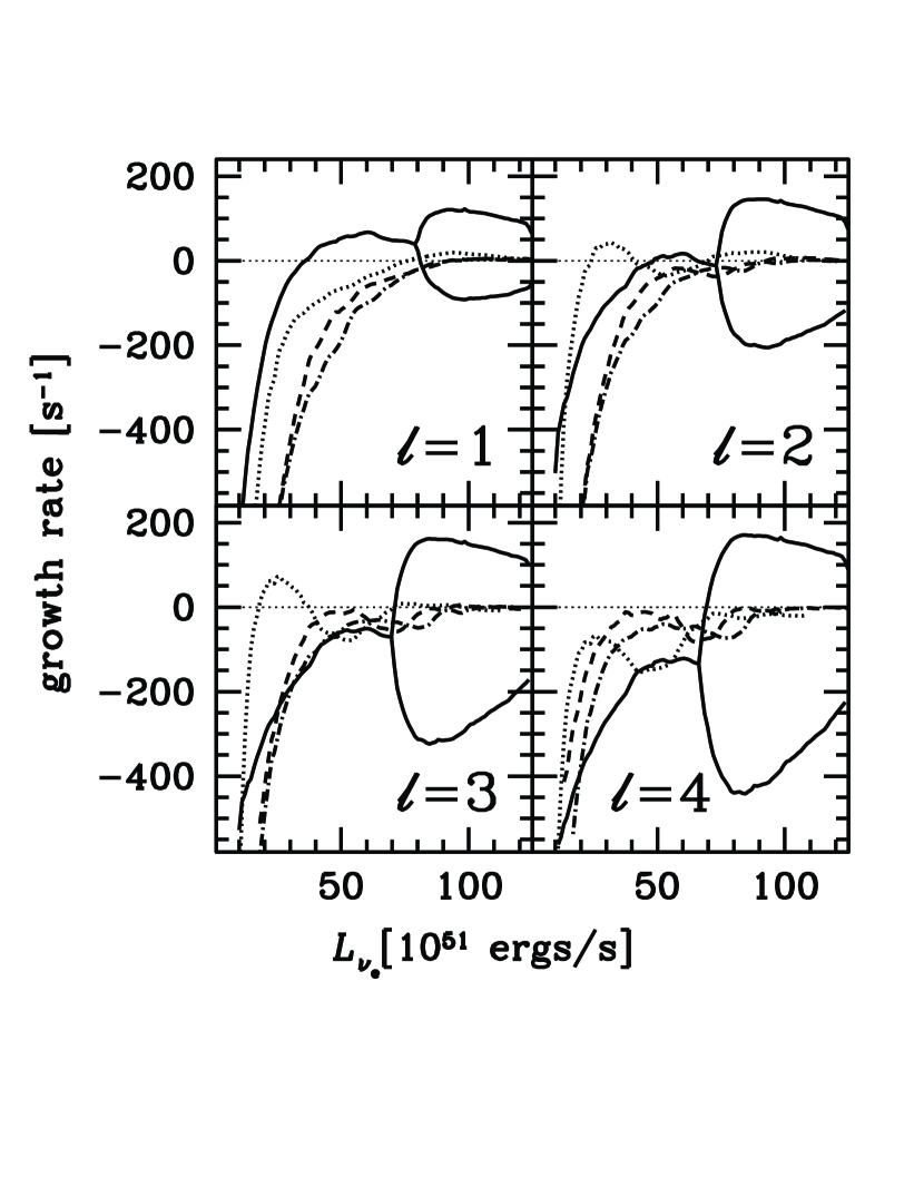
Figure 2: The growth rates, ${\rm Re}(\omega)$, for the non-radial modes of $\ell=1,2,3,4$ as a function of neutrino luminosity. The solid curves represent the fundamental modes while the dotted, dashed and dash-dotted curves correspond to the first, second and third overtones, respectively.

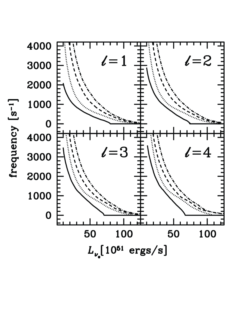
Figure 3: The oscillation frequencies, ${\rm Im}(\omega)$, the non-radial modes of $\ell=1,2,3,4$ as a function of neutrino luminosity. The solid curves represent the fundamental modes while the dotted, dashed and dash-dotted curves correspond to the first, second and third overtones, respectively.

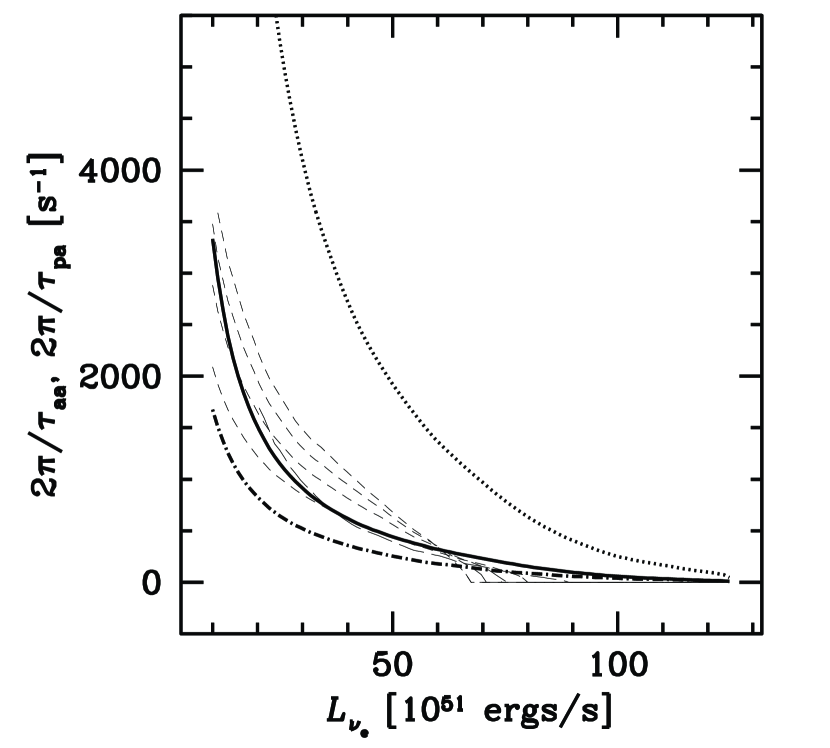
Figure 4: The characteristic frequencies of the advection-acoustic cycle, $2\pi/\tau_{\rm aa}$, and purely acoustic cycle, $2\pi/\tau_{\rm pa}$, together with the oscillation frequencies for some modes. The solid curve shows $2\pi/\tau_{\rm aa}$ while the dotted curve gives $2\pi/\tau_{\rm pa}$. The thin dashed curves represent the oscillation frequencies for the radial (long dashed curve) and non-radial fundamental modes of $\ell=1,2,3,4$ from bottom to top for low neutrino luminosities. The dash-dotted curve presents the characteristic frequency for the round trip along the shock front for the sound wave.

We solved these equations for a wide range of the control parameters, that is, the mass accretion rate and neutrino luminosity. The results were shown in Figs. 2-4 in Yamasaki & Yamada (2006). It is just repeated that there is a critical luminosity for each given mass accretion rate, above which there exists no steady solution.

2.2 Basic Equations for Perturbations

The formulation is essentially based on the spherical coordinates ($r$, $\theta$, $\phi$). In order to treat a variable outer boundary position, however, we adopt a new variable $x$ instead of $r$ as follows,

$$x=\frac{r-r_{\nu}}{r_{\rm s}-r_{\nu}},$$ (1)

where $r_{\rm s}$ and $r_{\nu}$ denote, respectively, the radii of the shock front and of the inner boundary, which corresponds to the neutrino sphere. The time-dependent Euler equations are expressed as

$$\frac{\partial\rho}{\partial t}-\frac{x}{r_{\rm s}-r_{\nu}}\frac{\partial r_{\rm s}}{\partial t}\frac{\partial\rho}{\partial x}+\frac{\rho}{r_{\rm s}-r_{\nu}}\frac{\partial u_{r}}{\partial x}+\frac{u_{r}}{r_{\rm s}-r_{\nu}}\frac{\partial\rho}{\partial x}$$ (2)

$$+\frac{2\rho u_{r}}{r}+\frac{\rho}{r}\frac{\partial u_{\theta}}{\partial\theta}+\frac{\cot\theta\rho u_{\theta}}{r}+\frac{\rho}{r\sin\theta}\frac{\partial u_{\phi}}{\partial\phi}=0,$$

$$\frac{\partial u_{r}}{\partial t}-\frac{x}{r_{\rm s}-r_{\nu}}\frac{\partial r_{\rm s}}{\partial t}\frac{\partial u_{r}}{\partial x}+\frac{u_{r}}{r_{\rm s}-r_{\nu}}\frac{\partial u_{r}}{\partial x}+\frac{1}{r_{\rm s}-r_{\nu}}\frac{1}{\rho}\frac{\partial p}{\partial x}+\frac{GM}{r^{2}}=0,$$ (3)

$$\frac{\partial u_{\theta}}{\partial t}+\frac{u_{r}}{r_{\rm s}-r_{\nu}}\frac{\partial u_{\theta}}{\partial x}+\frac{u_{r}u_{\theta}}{r}+\frac{1}{r\rho}\frac{\partial p}{\partial\theta}-\frac{1}{r\rho}\frac{x}{r_{\rm s}-r_{\nu}}\frac{\partial r_{\rm s}}{\partial\theta}\frac{\partial p}{\partial x}=0,$$ (4)

$$\frac{\partial u_{\phi}}{\partial t}+\frac{u_{r}}{r_{\rm s}-r_{\nu}}\frac{\partial u_{\phi}}{\partial x}+\frac{u_{r}u_{\phi}}{r}+\frac{1}{r\rho}\frac{\partial p}{\partial\phi}-\frac{1}{r\rho}\frac{x}{r_{\rm s}-r_{\nu}}\frac{\partial r_{\rm s}}{\partial\phi}\frac{\partial p}{\partial x}=0,$$ (5)

$$\frac{\partial S}{\partial t}-\frac{x}{r_{\rm s}-r_{\nu}}\frac{\partial r_{\rm s}}{\partial t}\frac{\partial S}{\partial x}+\frac{u_{r}}{r_{\rm s}-r_{\nu}}\frac{\partial S}{\partial x}=\frac{\dot{q}}{\rho T},$$ (6)

$$\frac{\partial Y_{e}}{\partial t}-\frac{x}{r_{\rm s}-r_{\nu}}\frac{\partial r_{\rm s}}{\partial t}\frac{\partial Y_{e}}{\partial x}+\frac{u_{r}}{r_{\rm s}-r_{\nu}}\frac{\partial Y_{e}}{\partial x}=\frac{\lambda}{n},$$ (7)

where $u_{r}$, $u_{\theta}$, $u_{\phi}$ stand for the velocity components and $\rho$, $p$, $S$, $Y_{e}$ and $n$ represent the density, pressure, entropy per unit mass, electron fraction and baryon number density, respectively; $G$ is the gravitational constant and $\dot{M}$ is the mass accretion rate, which is also constant in time; $M$ is the enclosed mass; $\dot{q}$ and $\lambda$ are the net heating and reaction rates for the absorptions and emissions of neutrinos on free nucleons. The terms originating from the non-orthogonality of the new coordinate system are dropped here because they are of higher order in terms of the deviation from the steady solution.

The formulation is again Newtonian and the rotation and magnetic field were neglected. Since the perturbed flows are also optically thin for neutrinos in the region of interest, the neutrino transport was ignored. In addition, we neglected the perturbations of the self-gravity of the accretion flows. This is justified from the fact that the inclusion of the self-gravity did not change much the unperturbed steady solutions except for the case with the neutrino luminosity very close to the critical value (see figure 3b in Yamasaki & Yamada (2006)). As will become clear later, the latter case is of no importance in reality.

The Rankine-Hugoniot relations at the outer boundary are expressed as

$$\rho({\bf u}-{\bf u}_{\rm s})\cdot{\bf n}=\rho_{\rm u}({\bf u}_{\rm u}-{\bf u}_{\rm s})\cdot{\bf n},$$ (8)

$$({\bf u}-{\bf u}_{\rm s})\cdot{\bf t}_{\alpha}=({\bf u}_{\rm u}-{\bf u}_{\rm s})\cdot{\bf t}_{\alpha},$$ (9)

$$({\bf u}-{\bf u}_{\rm s})\cdot{\bf t}_{\beta}=({\bf u}_{\rm u}-{\bf u}_{\rm s})\cdot{\bf t}_{\beta},$$ (10)

$$\rho\left\{({\bf u}-{\bf u}_{\rm s})\cdot\frac{\bf n}{|{\bf n}|}\right\}^{2}+p=\rho_{\rm u}\left\{({\bf u}_{\rm u}-{\bf u}_{\rm s})\cdot\frac{\bf n}{|{\bf n}|}\right\}^{2}+p_{\rm u},$$ (11)

$$\frac{1}{2}\left\{({\bf u}-{\bf u}_{\rm s})\cdot\frac{\bf n}{|{\bf n}|}\right\}^{2}+\epsilon+\frac{p}{\rho}=\frac{1}{2}\left\{({\bf u}_{\rm u}-{\bf u}_{\rm s})\cdot\frac{\bf n}{|{\bf n}|}\right\}^{2}+\epsilon_{\rm u}+\frac{p_{\rm u}}{\rho_{\rm u}},$$ (12)

where ${\bf u}_{\rm s}$ and $\epsilon$ are the shock velocity and specific internal energy, respectively; The suffix ${\rm u}$ stands for the quantities in the upstream, which was assumed to be free fall and cold; The vectors normal and tangent to the shock surface are denoted as ${\bf n}$ and ${\bf t}_{\alpha}$, ${\bf t}_{\beta}$, respectively, and are given as

$${\bf n}=\left(1,-\frac{1}{r_{\rm s}}\frac{\partial r_{\rm s}}{\partial\theta},-\frac{1}{r_{\rm s}\sin\theta}\frac{\partial r_{\rm s}}{\partial\phi}\right),$$ (13)

$${\bf t}_{\alpha}=\left(\frac{\partial r_{\rm s}}{\partial\theta},r_{\rm s},0\right),$$ (14)

$${\bf t}_{\beta}=\left(\frac{1}{\sin\theta}\frac{\partial r_{\rm s}}{\partial\phi},0,r_{\rm s}\right).$$ (15)

For the linear analysis, we employed the formulation based on the Eulerian perturbation at the fixed $x$-coordinate. The deviations from the unperturbed states are expanded with the spherical harmonics, $Y_{\ell}^{m}(\theta,\phi)$, and are assumed to have a time dependence of $\exp(\omega t)$. Attaching the subscript $0$ to the unperturbed variables and the subscript $1$ to the deviations from them of the perturbed counterparts, we expressed, for example, the radial velocity as

$$u_{r}=u_{r0}(x)+\sum_{\ell,m}u_{r1}(x)Y_{\ell}^{m}(\theta,\phi)\,e^{\omega t}.$$ (16)

The exceptions are $u_{\theta}$ and $u_{\phi}$, which were expanded with the vector spherical harmonics as

$$\left(\begin{array}[]{c}u_{\theta}\\ u_{\phi}\end{array}\right)=\sum_{\ell,m}u_{h1}(x)\left(\begin{array}[]{c}\displaystyle{\frac{\partial Y_{\ell}^{m}(\theta,\phi)}{\partial\theta}}\\ \displaystyle{\frac{\partial Y_{\ell}^{m}(\theta,\phi)}{\sin\theta\,\partial\phi}}\end{array}\right)\,e^{\omega t}.$$ (17)

Then the basic equations describing the perturbations to the lowest order are given for each $\ell$ as follows:

$$\frac{d(\rho_{1}/\rho_{0})}{dx}+\frac{d(u_{r1}/u_{r0})}{dx}+\frac{r_{{\rm s}0}-r_{\nu}}{u_{r0}}\omega\frac{\rho_{1}}{\rho_{0}}-\ell(\ell+1)\frac{r_{{\rm s}0}-r_{\nu}}{r}\frac{u_{h1}}{u_{r0}}$$ (18)

$$-\left[\left(\frac{d\ln\rho_{0}}{dx}+\frac{d\ln|u_{r0}|}{dx}\right)\frac{r_{{\rm s}0}}{r_{{\rm s}0}-r_{\nu}}+\left\{\frac{\omega}{u_{r0}}\frac{d\ln\rho_{0}}{dx}+\frac{2(r_{{\rm s}0}-r_{\nu})}{r^{2}}\right\}xr_{{\rm s}0}\right]\frac{r_{{\rm s}1}}{r_{{\rm s}0}}=0,$$

$$\frac{d(u_{r1}/u_{r0})}{dx}+\frac{p_{0}}{u_{r0}^{2}\rho_{0}}\left(\frac{\partial\ln p}{\partial\ln\rho}\right)_{0}\frac{d(\rho_{1}/\rho_{0})}{dx}+\frac{p_{0}}{u_{r0}^{2}\rho_{0}}\left(\frac{\partial\ln p}{\partial\ln S}\right)_{0}\frac{d(S_{1}/S_{0})}{dx}+\frac{p_{0}}{u_{r0}^{2}\rho_{0}}\left(\frac{\partial\ln p}{\partial\ln Y_{e}}\right)_{0}\frac{d(Y_{e1}/Y_{e0})}{dx}$$ (19)

$$+\left(\frac{r_{{\rm s}0}-r_{\nu}}{u_{r0}}\omega+2\frac{d\ln|u_{r0}|}{dx}\right)\frac{u_{r1}}{u_{r0}}+\left\{\frac{d\ln\rho_{0}}{dx}\frac{\rho_{0}^{2}}{p_{0}}\left(\frac{\partial^{2}p}{\partial\rho^{2}}\right)_{0}-\left(\frac{\partial\ln p}{\partial\ln S}\right)_{0}\frac{d\ln S_{0}}{dx}\right.$$

$$+\left.\frac{d\ln S_{0}}{dx}\frac{\rho_{0}S_{0}}{p_{0}}\left(\frac{\partial^{2}p}{\partial\rho\partial S}\right)_{0}-\left(\frac{\partial\ln p}{\partial\ln Y_{e}}\right)_{0}\frac{d\ln Y_{e0}}{dx}+\frac{d\ln Y_{e0}}{dx}\frac{\rho_{0}Y_{e0}}{p_{0}}\left(\frac{\partial^{2}p}{\partial\rho\partial Y_{e}}\right)_{0}\right\}\frac{p_{0}}{u_{r0}^{2}\rho_{0}}\frac{\rho_{1}}{\rho_{0}}$$

$$+\left\{\frac{d\ln\rho_{0}}{dx}\frac{\rho_{0}S_{0}}{p_{0}}\left(\frac{\partial^{2}p}{\partial\rho\partial S}\right)_{0}+\left(\frac{\partial\ln p}{\partial\ln S}\right)_{0}\frac{d\ln S_{0}}{dx}\right.+\left.\frac{d\ln S_{0}}{dx}\frac{S_{0}^{2}}{p_{0}}\left(\frac{\partial^{2}p}{\partial S^{2}}\right)_{0}\right.$$

$$+\left.\frac{d\ln Y_{e0}}{dx}\frac{S_{0}Y_{e0}}{p_{0}}\left(\frac{\partial^{2}p}{\partial S\partial Y_{e}}\right)_{0}\right\}\frac{p_{0}}{u_{r0}^{2}\rho_{0}}\frac{S_{1}}{S_{0}}$$

$$+\left\{\frac{d\ln\rho_{0}}{dx}\frac{\rho_{0}Y_{e0}}{p_{0}}\left(\frac{\partial^{2}p}{\partial\rho\partial Y_{e}}\right)_{0}+\frac{d\ln S_{0}}{dx}\frac{S_{0}Y_{e0}}{p_{0}}\left(\frac{\partial^{2}p}{\partial S\partial Y_{e}}\right)_{0}+\left(\frac{\partial\ln p}{\partial\ln Y_{e}}\right)_{0}\frac{d\ln Y_{e0}}{dx}\right.$$

$$\left.+\frac{d\ln Y_{e0}}{dx}\frac{Y_{e0}^{2}}{p_{0}}\left(\frac{\partial^{2}p}{\partial Y_{e}^{2}}\right)_{0}\right\}\frac{p_{0}}{u_{r0}^{2}\rho_{0}}\frac{Y_{e1}}{Y_{e0}}$$

$$-\left\{\frac{\omega}{u_{r0}}\frac{d\ln|u_{r0}|}{dx}+\frac{2(r_{{\rm s}0}-r_{\nu})GM}{r^{3}u_{r0}^{2}}\right\}xr_{{\rm s}0}\frac{r_{{\rm s}1}}{r_{{\rm s}0}}$$

$$-\left[\frac{d\ln|u_{r0}|}{dx}+\left\{\left(\frac{\partial\ln p}{\partial\ln\rho}\right)_{0}\frac{d\ln\rho_{0}}{dx}+\left(\frac{\partial\ln p}{\partial\ln S}\right)_{0}\frac{d\ln S_{0}}{dx}+\left(\frac{\partial\ln p}{\partial\ln Y_{e}}\right)_{0}\frac{d\ln Y_{e0}}{dx}\right\}\frac{p_{0}}{u_{r0}^{2}\rho_{0}}\right]$$

$$\times\frac{r_{{\rm s}0}}{r_{{\rm s}0}-r_{\nu}}\frac{r_{{\rm s}1}}{r_{{\rm s}0}}=0,$$

$$\frac{d(u_{h1}/u_{0})}{dx}+\left(\frac{r_{{\rm s}0}-r_{\nu}}{u_{r0}}\omega+\frac{r_{{\rm s}0}-r_{\nu}}{r}+\frac{d\ln|u_{r0}|}{dx}\right)\frac{u_{h1}}{u_{r0}}$$ (20)

$$+\frac{r_{{\rm s}0}-r_{\nu}}{r}\frac{p_{0}}{u_{r0}^{2}\rho_{0}}\left\{\left(\frac{\partial\ln p}{\partial\ln\rho}\right)_{0}\frac{\rho_{1}}{\rho_{0}}+\left(\frac{\partial\ln p}{\partial\ln S}\right)_{0}\frac{S_{1}}{S_{0}}+\left(\frac{\partial\ln p}{\partial\ln Y_{e}}\right)_{0}\frac{Y_{e1}}{Y_{e0}}\right\}$$

$$-\frac{1}{r}\frac{p_{0}}{u_{r0}^{2}\rho_{0}}\frac{d\ln p_{0}}{dx}xr_{{\rm s}0}\frac{r_{{\rm s}1}}{r_{{\rm s}0}}=0\quad\qquad(\mbox{for $\ell\neq 0$}),$$

$$\frac{d(S_{1}/S_{0})}{dx}-\frac{r_{{\rm s}0}-r_{\nu}}{S_{0}u_{r0}\rho_{0}T_{0}}\left\{\rho_{0}\left(\frac{\partial\dot{q}}{\partial\rho}\right)_{0}-\left(\frac{\partial\ln T}{\partial\ln\rho}\right)_{0}\dot{q}_{0}-\dot{q}_{0}\right\}\frac{\rho_{1}}{\rho_{0}}+\frac{d\ln S_{0}}{dx}\frac{u_{r1}}{u_{r0}}$$ (21)

$$+\left[\frac{r_{{\rm s}0}-r_{\nu}}{u_{r0}}\omega+\frac{d\ln S_{0}}{dx}-\frac{r_{{\rm s}0}-r_{\nu}}{S_{0}u_{r0}\rho_{0}T_{0}}\left\{S_{0}\left(\frac{\partial\dot{q}}{\partial S}\right)_{0}-\left(\frac{\partial\ln T}{\partial\ln S}\right)_{0}\dot{q}_{0}\right\}\right]\frac{S_{1}}{S_{0}}$$

$$-\frac{r_{{\rm s}0}-r_{\nu}}{S_{0}u_{r0}\rho_{0}T_{0}}\left\{Y_{e0}\left(\frac{\partial\dot{q}}{\partial Y_{e}}\right)_{0}-\left(\frac{\partial\ln T}{\partial\ln Y_{e}}\right)_{0}\dot{q}_{0}\right\}\frac{Y_{e1}}{Y_{e0}}$$

$$-\left\{\frac{d\ln S_{0}}{dx}\frac{r_{{\rm s}0}}{r_{{\rm s}0}-r_{\nu}}+\left(\frac{\omega}{u_{r0}}\frac{d\ln S_{0}}{dx}+\frac{r_{{\rm s}0}-r_{\nu}}{S_{0}u_{r0}\rho_{0}T_{0}}\frac{\partial\dot{q}_{0}}{\partial r}\right)xr_{{\rm s}0}\right\}\frac{r_{{\rm s}1}}{r_{{\rm s}0}}$$

$$-\frac{r_{{\rm s}0}-r_{\nu}}{S_{0}u_{r0}\rho_{0}T_{0}}T_{\nu 0}\left(\frac{\partial\dot{q}}{\partial T_{\nu}}\right)_{0}\frac{T_{\nu 1}}{T_{\nu 0}}=0,$$

$$\frac{d(Y_{e1}/Y_{e0})}{dx}+\frac{d\ln Y_{e0}}{dx}\frac{u_{r1}}{u_{r0}}-\frac{r_{{\rm s}0}-r_{\nu}}{Y_{e0}n_{0}u_{r0}}\rho_{0}\left(\frac{\partial\lambda}{\partial\rho}\right)_{0}\frac{\rho_{1}}{\rho_{0}}-\frac{r_{{\rm s}0}-r_{\nu}}{Y_{e0}n_{0}u_{r0}}S_{0}\left(\frac{\partial\lambda}{\partial S}\right)_{0}\frac{S_{1}}{S_{0}}$$ (22)

$$+\left\{\frac{r_{{\rm s}0}-r_{\nu}}{u_{r0}}\omega+\frac{d\ln Y_{e0}}{dx}-\frac{r_{{\rm s}0}-r_{\nu}}{Y_{e0}n_{0}u_{r0}}Y_{e0}\left(\frac{\partial\lambda}{\partial Y_{e}}\right)_{0}\right\}\frac{Y_{e1}}{Y_{e0}}$$

$$-\left\{\left(\frac{\omega}{u_{r0}}\frac{d\ln Y_{e0}}{dx}+\frac{r_{{\rm s}0}-r_{\nu}}{Y_{e0}n_{0}u_{r0}}\frac{\partial\lambda_{0}}{\partial r}\right)xr_{{\rm s}0}+\frac{d\ln Y_{e0}}{dx}\frac{r_{{\rm s}0}}{r_{{\rm s}0}-r_{\nu}}\right\}\frac{r_{{\rm s}1}}{r_{{\rm s}0}}$$

$$-\frac{r_{{\rm s}0}-r_{\nu}}{Y_{e0}n_{0}u_{r0}}T_{\nu 0}\left(\frac{\partial\lambda}{\partial T_{\nu}}\right)_{0}\frac{T_{\nu 1}}{T_{\nu 0}}+\frac{r_{{\rm s}0}-r_{\nu}}{Y_{e0}n_{0}u_{r0}}\lambda_{0}\frac{n_{1}}{n_{0}}=0,$$

where $T$ and $T_{\nu}$ denote the temperatures of matter and neutrino, respectively. The eigen values are degenerate in $m$ for the spherically symmetric background. The index $\ell$ explicitly appears only in Eq. (18).

The Rankine-Hugoniot relations for the perturbed quantities are written down similarly as

$$(2\rho_{{\rm f}0}u_{{\rm f}0}+\omega r_{{\rm s}0}\rho_{{\rm f}0}-\omega r_{{\rm s}0}\rho_{0})\frac{r_{{\rm s}1}}{r_{{\rm s}0}}+\rho_{0}u_{r0}\left(\frac{\rho_{1}}{\rho_{0}}+\frac{u_{r1}}{u_{r0}}\right)=0,$$ (23)

$$\frac{u_{h1}}{u_{r0}}-\left(\frac{u_{{\rm f}0}}{u_{r0}}-1\right)\frac{r_{{\rm s}1}}{r_{{\rm s}0}}=0\quad\qquad(\mbox{for $\ell\neq 0$}),$$ (24)

$$\left\{\frac{5}{2}\rho_{{\rm f}0}u_{\rm f0}^{2}+2\omega r_{{\rm s}0}\rho_{{\rm f}0}u_{{\rm f}0}-2\omega r_{{\rm s}0}\rho_{0}u_{r0}+\frac{3}{2}\rho_{{\rm f}0}\left(\frac{\partial p}{\partial\rho}\right)_{{\rm f}0}\right\}\frac{r_{{\rm s}1}}{r_{{\rm s}0}}$$ (25)

$$+2\rho_{0}u_{0}^{2}\frac{u_{r1}}{u_{r0}}+\left\{\rho_{0}u_{r0}^{2}+\rho_{0}\left(\frac{\partial p}{\partial\rho}\right)_{0}\right\}\frac{\rho_{1}}{\rho_{0}}+S_{0}\left(\frac{\partial p}{\partial S}\right)_{0}\frac{S_{1}}{S_{0}}+Y_{e0}\left(\frac{\partial p}{\partial Y_{e}}\right)_{0}\frac{Y_{e1}}{Y_{e0}}=0,$$

$$\left\{\frac{1}{2}u_{{\rm f}0}^{2}+\omega r_{{\rm s}0}u_{{\rm f}0}-\omega r_{{\rm s}0}u_{r0}+\frac{3}{2}\rho_{{\rm f}0}\left(\frac{\partial\epsilon}{\partial\rho}\right)_{{\rm f}0}+\frac{3}{2}\left(\frac{\partial p}{\partial\rho}\right)_{{\rm f}0}-\frac{3}{2}\frac{p_{{\rm f}0}}{\rho_{{\rm f}0}}\right\}\frac{r_{{\rm s}1}}{r_{{\rm s}0}}$$ (26)

$$+u_{r0}^{2}\frac{u_{r1}}{u_{r0}}+\left\{\rho_{0}\left(\frac{\partial\epsilon}{\partial\rho}\right)_{0}+\left(\frac{\partial p}{\partial\rho}\right)_{0}-\frac{p_{0}}{\rho_{0}}\right\}\frac{\rho_{1}}{\rho_{0}}+\left\{S_{0}\left(\frac{\partial\epsilon}{\partial S}\right)_{0}+\frac{S_{0}}{\rho_{0}}\left(\frac{\partial p}{\partial S}\right)_{0}\right\}\frac{S_{1}}{S_{0}}$$

$$+\left\{Y_{e0}\left(\frac{\partial\epsilon}{\partial Y_{e}}\right)_{0}+\frac{Y_{e0}}{\rho_{0}}\left(\frac{\partial p}{\partial Y_{e}}\right)_{0}\right\}\frac{Y_{e1}}{Y_{e0}}=0.$$

Note that the upstream flows are unaffected by the perturbations inside the shock because they are supersonic and no fluctuations can propagate beyond the shock front. The suffix ${\rm f}0$ stands for the upstream values at the shock front for the free fall assumed in the unperturbed background state.

In addition, we imposed

$$u_{r1}=0,$$ (27)

at the inner boundary ($x=0$), considering that the infalling matter comes to rest on the neutron star surface that is supposed to be very close to the inner boundary; We did not try to obtain the ”unsteady” structure between the inner boundary and the neutron star surface where a thin boundary layer is formed, but chose instead to impose the boundary conditions for perturbations at the neutrino sphere although $u_{r0}\neq 0$ there, although we must impose the boundary condition at the top of the thin boundary layer between accretion flow and the neutron star surface, in principle. It is mentioned that as inferred from the detailed numerical simulations of the structure near the neutrino sphere (Liebendörfer et al., 2005), the distance between the neutrino sphere and the boundary layer is indeed much smaller than the typical wavelengths of the eigen modes we are concerned with. At the same time, the advection time from shock to the boundary layer is hardly altered by replacing the surface to the neutrino sphere; That is, the effect of the inner boundary is almost unchanged by the replacing. The effect of shifting the inner boundary will be discussed in § 5. Further, since the growth of SASI is expected to be affected by the imposed inner boundary conditions, we tried some variations of these conditions, the results of which will be discussed in § 5.

We solved Eqs. (18)-(22) as an eigen value problem for $\omega$, imposing the boundary conditions, Eqs. (23)-(27). The procedure is as follows. We first take a trial value of $\omega$, set $r_{{\rm s}1}/r_{{\rm s}0}$ to be unity and solve the Rankine-Hugoniot relations, Eqs. (23)-(26), and integrate Eqs. (18)-(22) from the outer boundary down to the inner boundary. The solution obtained this way does not, in general, meet the inner boundary condition, Eq. (27). Then we improve the value of $\omega$ and repeat the procedure until Eq. (27) is satisfied at the inner boundary by the solution.

3 Eigen Frequencies of Various Modes

In this section, we summarily present various modes that we found in this paper. The detailed analysis of each mode will be given in the following sections. We show only the results for $\dot{M}=1.0M_{\odot}/{\rm s}$, since their quantitative nature is weakly dependent on the value of mass accretion rate. Unlike in the previous paper (Yamasaki & Yamada, 2005), in this and next sections, the neutrino temperature is assumed to be unperturbed, that is, $T_{\nu 1}=0$. This is also equivalent to the negligence of the perturbation of neutrino luminosity. The underlying idea is that the neutrino luminosity is dominated by the contribution from the proto neutron star rather than from the accreted matter. The influence of the perturbation of neutrino luminosity will be considered separately in section 5. We explored all the modes of relevance below the critical neutrino luminosity, which is $124.801\times 10^{51}{\rm ergs/s}$ for the mass accretion rate given above.

First, we consider the radial modes with $\ell=0$. It is noted that the stability of spherical accretion flows against radial modes were investigated by several authors (Nakayama, 1992, 1993, 1994; Houck & Chevalier, 1992; Foglizzo & Tagger, 2000; Foglizzo, 2001, 2002; Galletti & Foglizzo, 2005; Yamasaki & Yamada, 2005) in different contexts. Nakayama (1992, 1993, 1994), for example, showed that the isothermal or adiabatic transonic accretion flows around black hole are unstable when the postshock flow is accelerated. The effect of cooling was investigated by Houck & Chevalier (1992) for the accretion flows to neutron stars or white dwarfs with a use of a simple analytic form of cooling. Yamasaki & Yamada (2005) analyzed the linear stability of spherically symmetric subsonic accretion flows from a standing shock down to a proto neutron star, using an analytic form of heating and cooling by neutrinos taken into account. This paper is an extention of Yamasaki & Yamada (2005) to the models with more realistic neutrino heating/cooling and equation of state that are appropriate for the post-bounce phase of core-collapse supernovae (see also Yamasaki & Yamada (2006)).

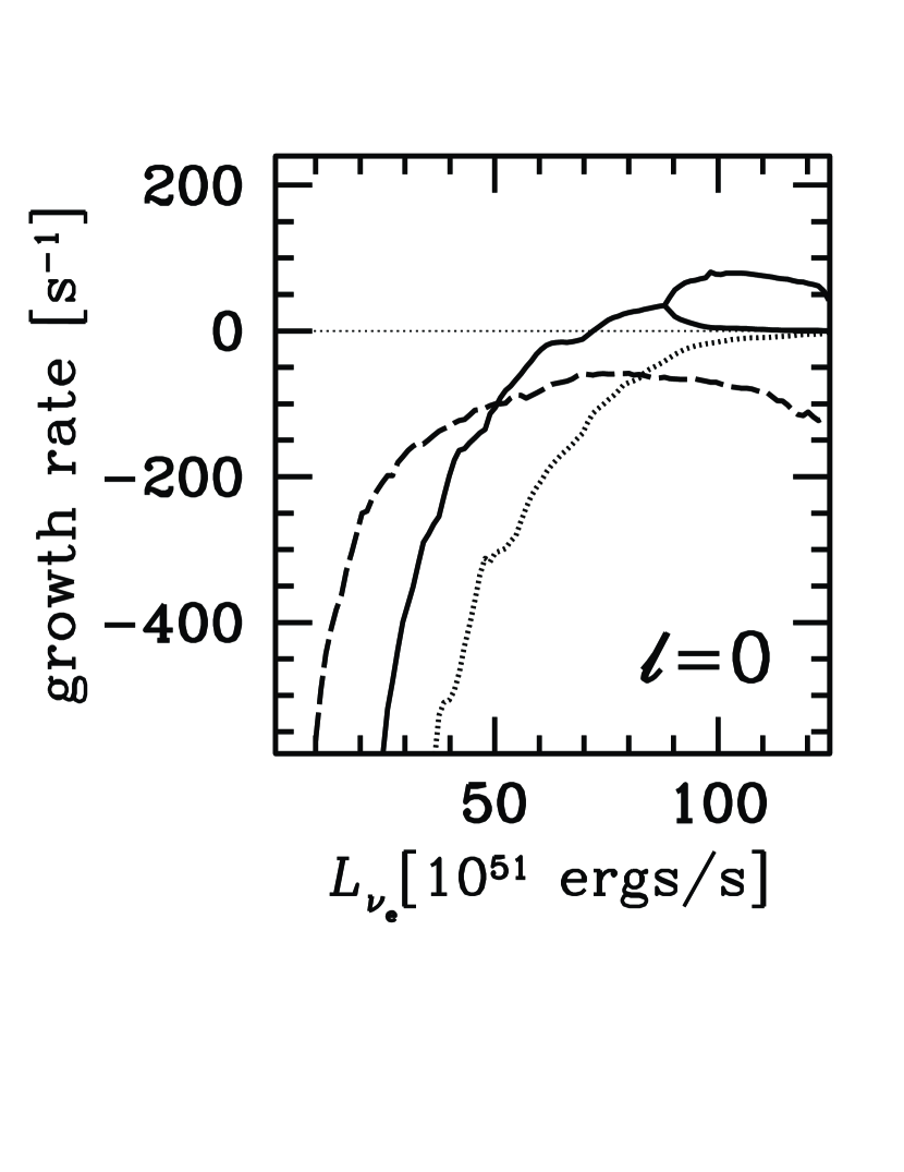
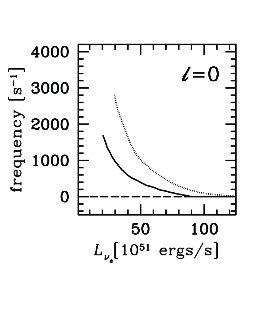
Figure 1: Left: The growth rates, ${\rm Re}(\omega)$, and Right: oscillation frequencies, ${\rm Im}(\omega)$, for representative radial ($\ell=0$) modes as a function of neutrino luminosity. The long dashed curve denotes the fundamental thermal mode. The solid and dotted curves correspond to the fundamental and first overtone oscillatory modes, respectively.

The results are shown in Fig. 1, where the real and imaginary parts of $\omega$ (see Eq. (16)) are displayed for representative radial modes. It is found from the right panel that there are both oscillatory (Im($\omega$)$\neq 0$) and non-oscillatory (Im($\omega$)$=0$) modes. The mode shown with a long-dashed line is non-oscillatory and stable (Re($\omega$)$<0$) for all the luminosities. We distinguish the eigen modes with similar features by the number of radial nodes. We refer to the eigen mode with the smallest number of radial nodes, normally none or one, as a fundamental mode of the family. The modes with the second and third smallest number of radial nodes are called the first and second overtones, respectively. In this notation, the above mentioned mode is a fundamental mode. This mode is of thermal nature in the sense that it disappears if the perturbations of the heating rates are neglected, and has no non-radial counterpart. This corresponds to the mode that was discussed in Yamasaki & Yamada (2005). It is interesting to point out that the mode is not unstable even marginally at the critical luminosity. This issue will be discussed further in detail in §5.

It is apparent from Fig. 1 that the radial stability is much more complicated in the present models than in those considered in Yamasaki & Yamada (2005). In fact, besides the thermal modes just discussed, we found oscillatory modes shown with solid and dashed lines in the figure. These are the fundamental and first overtone modes. This complexity is originated from the non-monotonic background flows obtained for the realistic neutrino heating rates and equation of state. We refer readers to Yamasaki & Yamada (2006) for more details on the unperturbed states. While the first overtone (the dotted line) is stable and oscillatory for all the luminosities up to the critical value, the fundamental mode becomes unstable when the luminosity is larger than $\sim 7\times 10^{52}{\rm ergs/s}$. For the luminosities greater than $\sim 9\times 10^{52}{\rm ergs/s}$, the mode bifurcates into two branches and become non-oscillatory. Although both the non-oscillatory modes are unstable, one of them is almost neutral for most of the luminosities. The overstablizing radial mode that exists for the luminosities $\lesssim 9\times 10^{52}{\rm ergs/s}$ was not found in Yamasaki & Yamada (2005) but observed in the numerical simulations by Ohnishi et al. (2006a) and the reason was not clear in the latter paper. (Note, however, that such overstablizing modes were found in their own models by Houck & Chevalier (1992), Galletti & Foglizzo (2005) and Blondin & Mezzacappa (2006).)

We can now ascribe the apparent discrepancy to the difference of the implemented microphysics. In fact, we re-examined the models with the simplified neutrino-heating rates and equation of state employed in Yamasaki & Yamada (2005) and found that the same mode exists in this case also indeed, but it is stable up to the critical luminosity. In Yamasaki & Yamada (2005), the critical luminosity was reached before the present mode becomes unstable. In other words, which mode becomes unstable for smaller neutrino luminosities, the present mode or the thermal mode, is dependent on the background model, which is in turn determined by the adopted microphysics. The oscillatory instability seems to be driven by the advection-acoustic cycles (Foglizzo & Tagger, 2000; Foglizzo, 2001, 2002). As shown in Fig. 4 together with other non-radial modes that will be discussed later, the oscillation frequency agrees with the period of the advection-acoustic cycle rather well. As will be described shortly, the non-radial modes become unstable for smaller neutrino luminosities than these radial unstable modes. Hence the latter modes will be of little practical importance. Other than the modes mentioned above, we did not find any unstable radial modes.

Next we pay attention to the stability of accretion flows against non-radial perturbations. Foglizzo & Tagger (2000); Foglizzo (2001, 2002) conducted linear analyses on the stability of black hole accretions, using a polytropic equation of state. They claimed that the origin of the instability is a repeated coupling of inward-advecting vortices and entropy perturbations with outward-propagating acoustic waves. It should be noted that the results cannot be directly applied to the post-bounce flows in the supernova core of our current interest. While in the the black hole accretion the flow is transonic and the inner boundary is the event horizon, in the latter case the flow is subsonic and there is a surface of proto neutron star at the inner boundary. Galletti & Foglizzo (2005) attempted a linear analysis more appropriate for the supernova core but with a polytopic equation of state and a simple analytic cooling term. Several numerical studies were also performed (Blondin et al., 2003; Scheck et al., 2004; Blondin & Mezzacappa, 2006; Ohnishi et al., 2006a), and they all found the growths of unstable modes with $\ell=1$ and $2$.

The results of our calculations are shown in Figs. 2 and 3, where the growth rates and oscillation frequencies of the fundamental and first three overtone modes are given for $\ell=1-4$. All the modes are oscillatory ($\rm{Im}(\omega)\neq 0$) for small neutrino luminosities $\lesssim 7\times 10^{52}{\rm ergs/s}$. The accretion flows are stable against all the non-radial modes if the neutrino luminosity is $\lesssim 1\times 10^{52}$ ergs/s for the present model with $\dot{M}=1.0M_{\odot}/{\rm s}$. For larger luminosities, the first overtones of $\ell=2$ and $3$ modes become unstable at first for relatively low neutrino luminosities, $2\sim 3\times 10^{52}$ ergs/s, whereas the fundamental modes with $\ell=1$ and $2$ become unstable for a bit higher luminosities, $3\sim 7\times 10^{52}$ ergs/s, with the former more unstable. For $\ell>3$, there is no unstable oscillatory mode. For still larger luminosities, $\gtrsim 7\times 10^{52}$ ergs/s, the fundamental modes of all $\ell$’s become non-oscillatory ($\rm{Im}(\omega)=0$) and unstable. It is interesting that they split into two different modes at the same neutrino luminosity. These features are quite similar to the radial fundamental modes, but are sensitive to the treatment of neutrino-luminositiy perturbations, which will be discussed in §5.

4 Mechanisms of Instabilities

We now discuss the nature of each mode more in detail. In the previous section, we found both oscillatory and non-oscillatory modes. In the following, we treat them separately.

4.1 Oscillatory Modes — Advection-Acoustic Cycle or Purely Acoustic Cycle?

As shown in the previous section, all the modes except for the radial fundamental thermal mode are oscillatory for low neutrino luminosities. Although most of them are decaying oscillators, some of them, e.g. the fundamental modes of $\ell=0,1$ and the first overtones of $\ell=2,3$ modes, become growing oscillators at a certain neutrino luminosity that is specific to each mode. Recently, Blondin & Mezzacappa (2006) and Ohnishi et al. (2006a) did 2D numerical experiments on the instability of the accretion flows onto a proto neutron star and observed the non-radial oscillatory instabilities. Moreover, they found the oscillating radial mode that had not been expected in the paper by Yamasaki & Yamada (2005) as mentioned in §3. Although the oscillation frequencies were consistent with each other, these authors preferred a different interpretation on the mechanism of the instabilities. While Ohnishi et al. (2006a) supported the advection-acoustic-cycle mechanism proposed by Foglizzo & Tagger (2000); Foglizzo (2001), Blondin & Mezzacappa (2006) claimed that the purely acoustic cycles were responsible for the instabilities. In order to shed light on this issue, we pay attention in this section to the possible origin of the oscillations.

We first compare a couple of frequencies of relevance. We define the time scales of the advection-acoustic cycle, $\tau_{\rm aa}$, and purely acoustic cycle, $\tau_{\rm pa}$, along the radial path as follows,

$$\tau_{\rm aa}\equiv\int^{r_{\rm s}}_{r_{\nu}}\left(\frac{1}{c_{s}+u_{r}}-\frac{1}{u_{r}}\right)dr,$$ (28)

$$\tau_{\rm pa}\equiv\int^{r_{\rm s}}_{r_{\nu}}\left(\frac{1}{c_{s}+u_{r}}+\frac{1}{c_{s}-u_{r}}\right)dr,$$ (29)

where $c_{s}$ is the sound speed. These frequencies are displayed together with the oscillation frequencies obtained for various modes in Fig. 4. We can see that $2\pi/\tau_{\rm aa}$, the characteristic frequency of the advection-acoustic cycle, agrees rather well with the oscillation frequencies of the radial and non-radial modes whereas the characteristic frequency for the acoustic cycle along the radial path, $2\pi/\tau_{\rm pa}$, is much larger. In fact, $\tau_{\rm aa}$ is almost coincident with the oscillation frequency of the radial oscillatory mode. Blondin & Mezzacappa (2006) insisted that the sound propagation is not radial for $\ell\neq 0$ modes. For comparison, we also calculated the characteristic frequency for the sound wave to travel around along the shock front although such a propagation of sound wave is highly unlikely, since the radial gradient of the sound velocity is negative and the sound wave will be deflected outwards like seismic waves. This frequency is in better agreement with the oscillation frequencies than $\tau_{\rm pa}$, but appears to be too small compared with the oscillation frequencies for low neutrino luminosities, particularly when the modes are unstable. For these low luminosities, the shock front is close to the inner boundary and the radial path is much shorter than the circular path, and, as a result, the difference of the interpretations is expected to be most remarkable. Note that the round-trip frequency becomes closer to the oscillation frequencies at the lowest luminosities. This is due to the non-monotonic radial dependence of sound velocity at these luminosities, where the vicinity of the shock front has the largest sound speed. These results, although not conclusive, seem to support the advection-acoustic-cycle origin of the oscillation frequencies

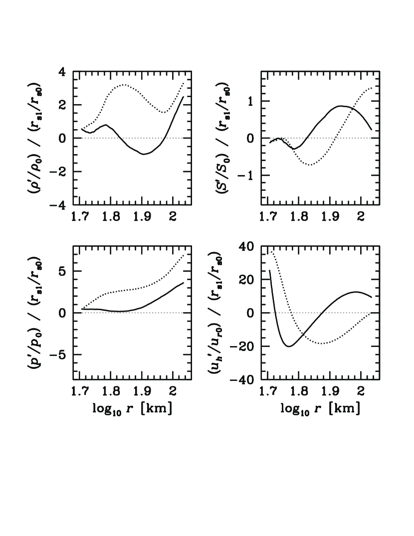
Figure 5: The eigen functions of the non-radial unstable mode with $\ell=1$ for $L_{\nu_{\rm e}}=6\cdot 10^{52}$ergs/s. The fundamental mode is shown. The solid and dotted curves represent the real and imaginary parts, respectively.

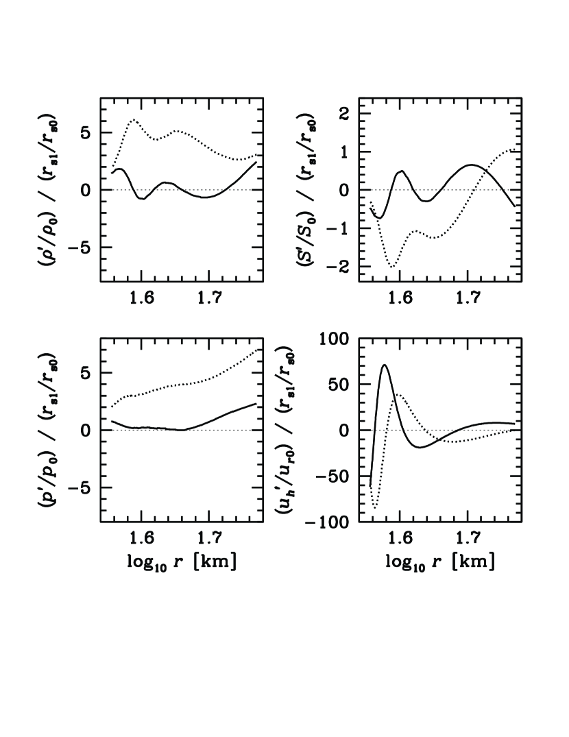
Figure 6: The eigen functions of the non-radial unstable mode with $\ell=2$ for $L_{\nu_{\rm e}}=3\cdot 10^{52}$ergs/s. The first overtone is shown. The solid and dotted curves represent the real and imaginary parts, respectively.

Next, we discuss whether the advection of entropy- and velocity perturbations and the propagation of pressure fluctuations actually occur in our models. In Figs. 5 and 6 shown are the eigen functions of the oscillatory modes of $\ell=1,2$. In drawing these figures, we changed the radial coordinate from $x$ to $r$ so that the Eulerian perturbations of variables for fixed $r$ could be obtained. For example, this Eulerian perturbation of $u_{r}$ denoted by the prime is related with another Eulerian perturbation for fixed $x$ by the following relation.

$$u^{\prime}_{r}\equiv u_{r1}-xr_{{\rm s}1}\frac{du_{r0}}{dr}.$$ (30)

Note that the luminosities are chosen so that the displayed modes are unstable, ${\rm Re}(\omega)>0$. The eigen functions are complex quantities in general and both the real and imaginary part are presented in the figures.

In order to see if a particular fluctuation is propagated inward or outward, we calculated the ”phase” of the perturbed quantity defined, for example, for the horizontal velocity as follows:

$$\phi\equiv\arccos\left(\frac{{\rm Re}(u_{h1})}{|u_{h1}|}\right).$$ (31)

The values within $[0,2\pi]$ are chosen at the shock front and extended continuously inwards.

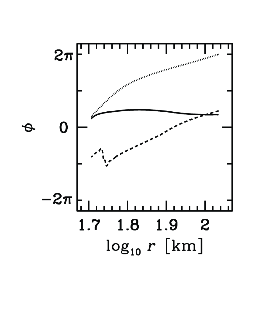
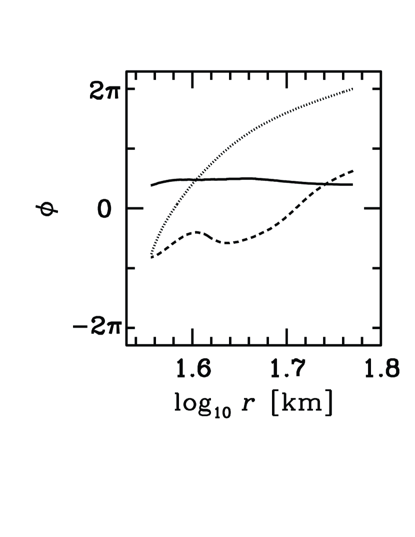
Figure 7: Left: The radial profiles of the phases of various perturbed quantities for the fundamental mode of $\ell=1$ at $L_{\nu_{\rm e}}=6\cdot 10^{52}$ergs/s. The solid, dotted and dashed curves represent the phases of pressure, horizontal velocity and entropy perturbations, respectively. Right: The same as in the left panel but for the first overtone of $\ell=2$ at $L_{\nu_{\rm e}}=3\cdot 10^{52}$ergs/s.

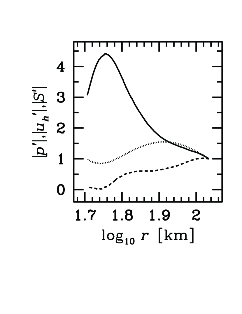
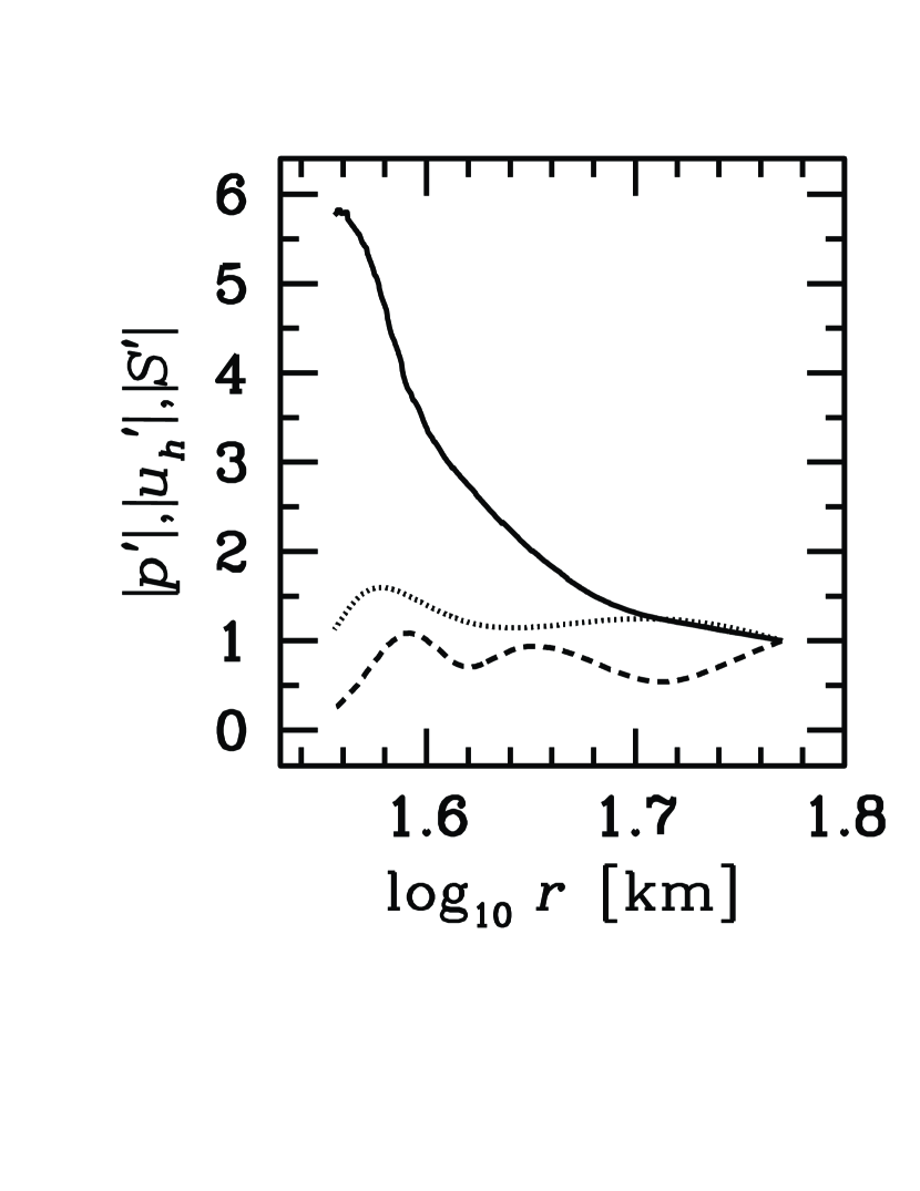
Figure 8: Left: The radial profiles of the amplitudes of various perturbed quantities for fundamental mode of $\ell=1$ at $L_{\nu_{\rm e}}=6\cdot 10^{52}$ergs/s. The notation is the same as in Fig. 7. The amplitudes are normalized at the shock front. Right: The same as in the left panel but for the first overtone of $\ell=2$ at $L_{\nu_{\rm e}}=3\cdot 10^{52}$ergs/s.

In Fig. 7 given are the phases of the perturbations of pressure, horizontal velocity and entropy. We also present the corresponding amplitudes in Fig. 8. It is clear from Fig. 7 that the phases of the perturbations of the horizontal velocity and entropy increase with radius, which implies that they are propagating inward. (Note that the perturbation is proportional to $\exp(i{\rm Im}(\omega)t)$). On the other hand, the phase of the pressure perturbation is almost constant with radius. There is a slight positive gradient in the inner region, indicating the inward propagation there, and a negative gradient in the outer region, implying the outward propagation. It should be also mentioned that the wave length of the pressure perturbations, that is the sound velocity times the oscillation frequency, is longer than the distance between the shock wave and the inner boundary. This is also reflected in the lack of short-wave-length modulations of the amplitude for the pressure perturbation shown in Figs. 5 and 6. In such a situation, it may not be meaningful to define a propagation path of the pressure perturbation and this might be the source of difficulty in interpreting the mechanism of the instability.

¿From Fig. 8, we can see which inward-advected quantity, the perturbation of entropy or horizontal velocity, could give a larger contribution to the excitation of pressure perturbations. Note that the amplitudes are normalized at the shock front. As is clear, the entropy perturbation is significantly damped from the initial value by the time it reaches the inner boundary. This is particularly the case for the fundamental mode of $\ell=1$ at $L_{\nu_{\rm e}}=6\cdot 10^{52}$ergs/s. The evolution of the entropy perturbation is determined by the non-adiabatic processes, that is the heating and cooling by neutrinos. A similar damping of the entropy perturbation is also seen for the first overtone of $\ell=2$ mode at $L_{\nu_{\rm e}}=3\cdot 10^{52}$ergs/s although the damping region is rather confined to the vicinity of the inner boundary. The perturbation of the horizontal velocity, on the other hand, is not reduced significantly as it is advected inward regardless of the unstable modes. Hence, if it is the advection-acoustic cycle that drives the instability, the vortices rather than the entropy fluctuations will be the dominant source of the excitation of pressure perturbations. It is incidentally mentioned that the pressure perturbation is also damped rather rapidly as it propagates outward as shown in Fig. 8.

It should be emphasized that pressure perturbations are generated at the inner boundary when vorteces arrive there if the solid boundary condition is imposed (Foglizzo et al., 2005). Since such pressure perturbations grow typically on the advection time scale, it can seriously affect the advection-acoustic cycle excited by the pressure perturbations produced physically outside the inner boundary if the advection time is comparable to the growth time of the cycle. The generations of pressure perturbations just on the inner boundary should be distinguished from those outside the boundary, the original excitation mechanism suggested by Foglizzo & Tagger (2000); Foglizzo (2001, 2002). We cannot tell, however, to what extent the former contaminates the latter and how for the present cases from the above analyses alone. We will discuss the issue in more detail in §5.

In our models meant for the core-collapse supernovae, the unstable modes induced supposedly by the vortex-acoustic cycle have lower oscillation frequencies compared with the models meant for the black hole accretion by Foglizzo (2001, 2002). This difference comes from the condition satisfied at the inner boundary, around which the excitation of acoustic waves takes place most efficiently. (See Foglizzo & Galletti (2004) for the physical interpretation.) Whereas the inflow velocity approaches the sound velocity at the inner boundary in the case of the black hole accretion, the flow is highly subsonic near the inner boundary in the present case, which lead to the observed lower frequencies of the unstable oscillations induced by advected vortices in our models.

4.2 Non-Oscillatory Modes — Convective Instability

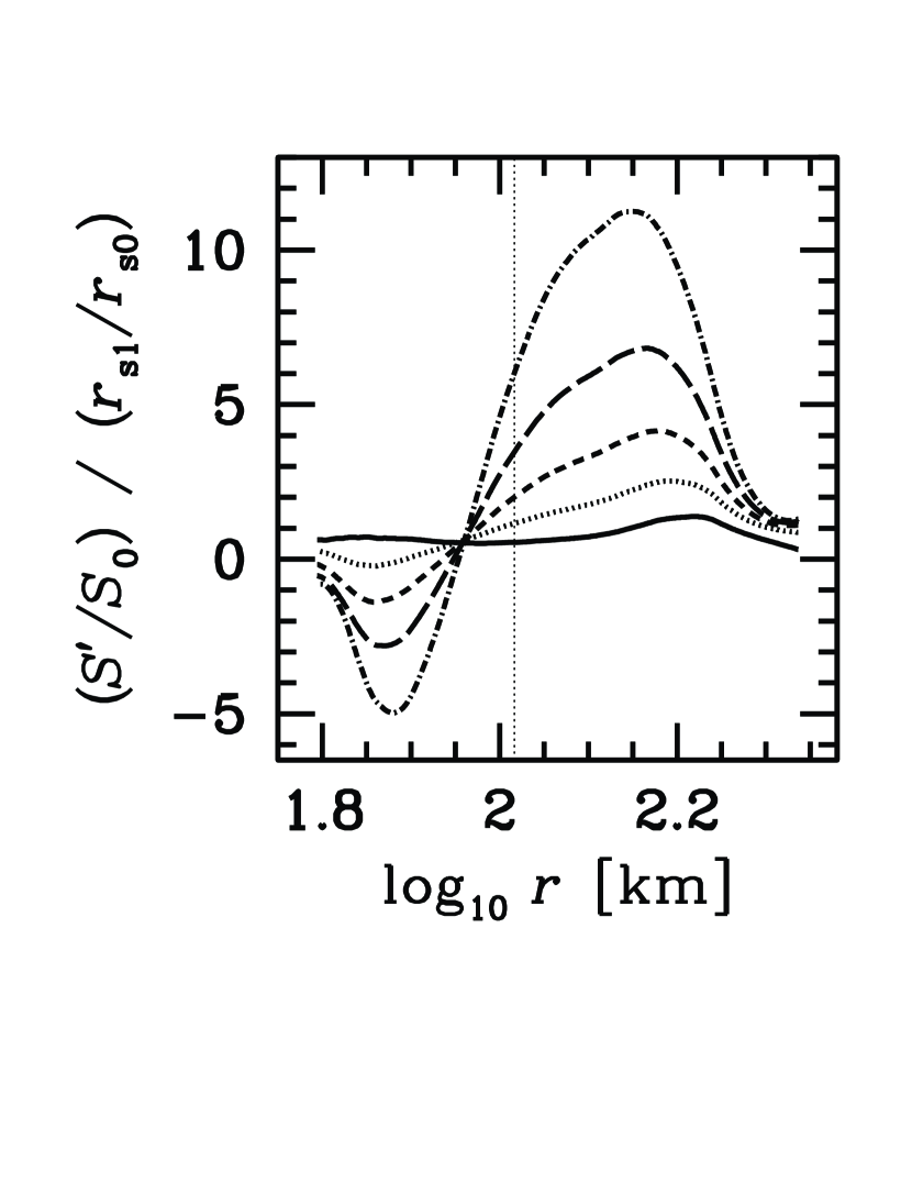
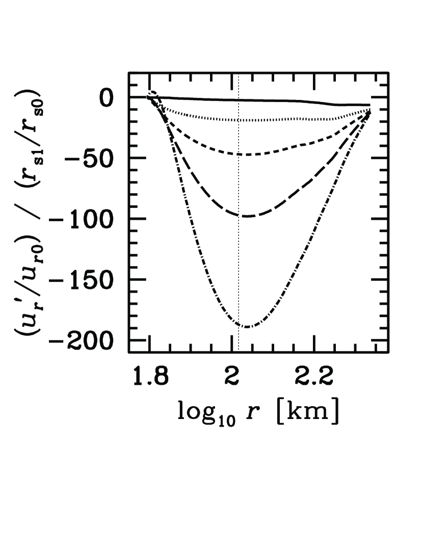
Figure 9: Left: The eigen functions of the entropy perturbation for non-oscillatory modes at $L_{\nu_{\rm e}}=9\cdot 10^{52}$ergs/s. The solid curve represents the radial model ($\ell=0$). The dotted, dashed, long dashed and dash-dotted curves correspond to the non-radial modes with $\ell=1,2,3,4$, respectively. Thin dotted line indicates the location of the gain radius. Right: The same as in the left panel but for the perturbation of radial velocity.

As shown in the previous section, when the luminosity is larger than about $7\times 10^{52}{\rm ergs/s}$, there exit non-oscillatory unstable modes for all $\ell$’s including $\ell=0$. (see Figs. 1 and 2.) Although the dependence of the growth rate on the neutrino luminosity looks similar for these unstable modes, the eigen functions of the non-radial modes ($\ell\neq 0$) are qualitatively different from that of the radial mode ($\ell=0$). This can be seen in Fig. 9, where the eigen functions of the modes with $\ell=0-4$ are displayed and the gain radius is marked by the thin dotted lines. While the eigen function of the entropy perturbation for the radial mode has no node, those for the non-radial modes have a node near the gain radius. The eigen functions of the radial-velocity perturbation also show a difference between them; they take the maximum absolute value near the gain radius for the non-radial modes, whereas a rather monotonic decay is seen for the radial mode as the radius decreases. The fact that the heating region between the shock and the gain radius has a negative entropy gradient and that these unstable non-radial modes appear to be excited in this region suggests that they are convective modes. (The radial mode cannot be the convective mode in nature).

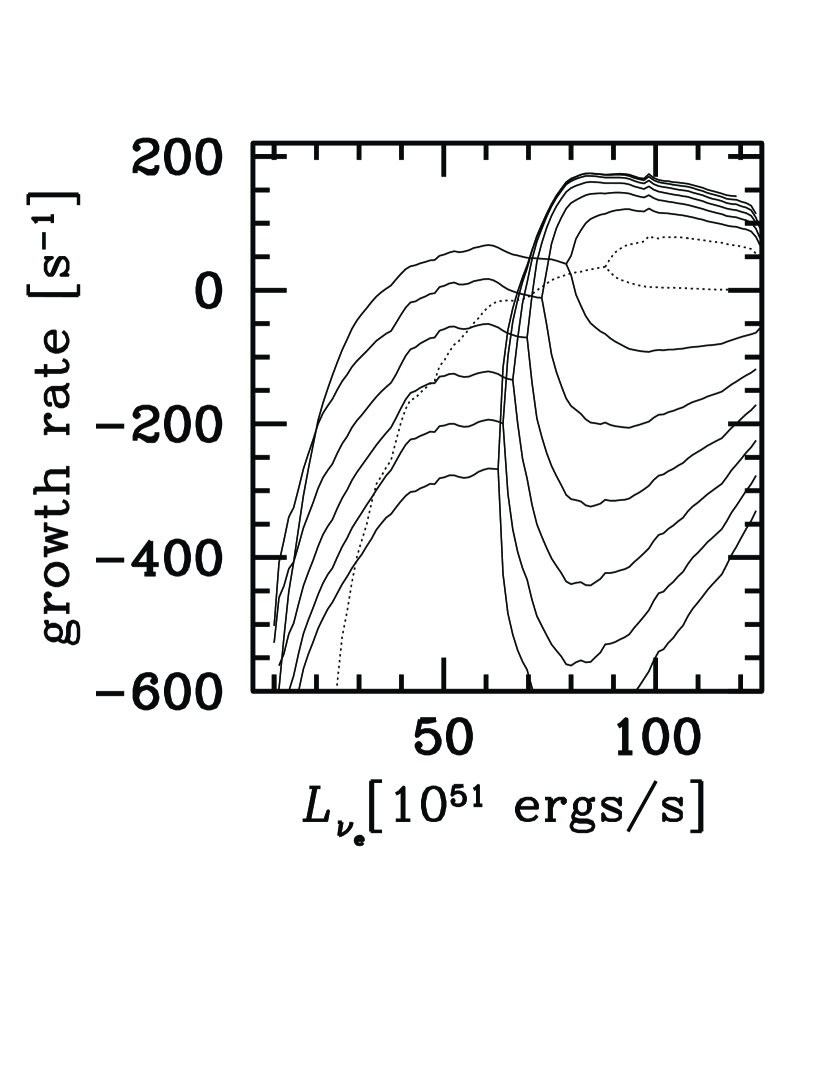
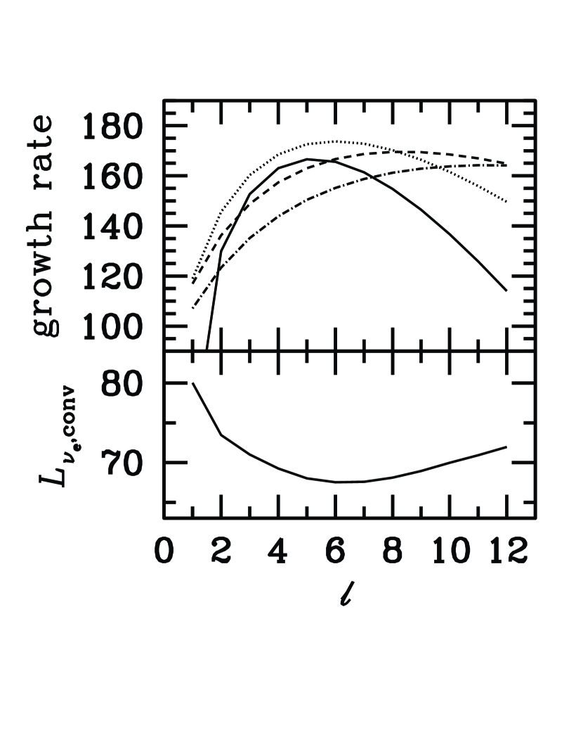
Figure 10: Left: The growth rates, ${\rm Re}(\omega)$, of the fundamental modes with different $\ell$’s. The solid curves represent the non-radial modes with $\ell=1-6$ from top to bottom at $L_{\nu_{\rm e}}=5\cdot 10^{52}$ergs/s. The dotted curve shows the radial mode ($\ell=0$). Top right: The growth rates, ${\rm Re}(\omega)$, of the unstable non-oscillatory modes (the upper branches of the bifurcated modes in the left panel) as a function of $\ell$. The solid, dotted, dashed and dash-dotted curve correspond to the results for $L_{\nu_{\rm e}}=8,9,10,11\cdot 10^{52}$ergs/s, respectively. Bottom right: The neutino luminosity in unit of $10^{51}$ergs/s, at which the convective mode with a given $\ell$ becomes unstable for the first time.

The growth rates of the convective modes together with the radial mode are demonstrated in Fig. 10. When the luminosity becomes greater than $\sim 7\times 10^{52}{\rm ergs/s}$, all the modes are bifurcated into two branches. Although this behavior is common to the radial mode, it is apparent from the left panel of this figure that the radial mode does not belong to the same family. In the right panels, the $\ell$-dependences of the growth rate (upper panel) and the luminosity (lower panel), at which the mode with a given $\ell$ becomes unstable for the first time, are shown. The growth rate increases at first and then decreases as $\ell$ becomes larger. The peak occurs at $\ell=5-11$, depending on the neutrino luminosity. On the other hand, the luminosity, at which the convective instability appears, decreases with $\ell$ at first until $\ell=6$ and then it increases. These peaks are rather broad, and a couple of modes become unstable almost at the same luminosity with similar growth rates.

As shown in the previous paper (Yamasaki & Yamada, 2005, 2006), there appears a heating region in the accretion flow for the luminosity larger than a certain value. It is easy to see that the heating region, if exists, has a negative entropy gradient. In such a region, the conventional criterion predicts an existence of convection. In our models with the mass accretion rate of $\dot{M}=1.0M_{\odot}/{\rm s}$, the critical luminosity for the existence of the heating region is $3.7\times 10^{52}{\rm ergs/s}$. It should be emphasized here that the actual convective instability occurred at larger neutrino luminosity, $\sim 7\times 10^{52}{\rm ergs/s}$. This confirms the recent findings by Foglizzo et al. (2006a) that the advection stabilizes the convective modes.

Introducing the parameter $\chi$, which is roughly the ratio of the advection time scale and the growth time scale of convective instability, Foglizzo et al. (2006a) gave the additional criterion, $\chi>3$, for the convective instability in the advecting matter. In our previous paper (Yamasaki & Yamada, 2006), we calculated the value of $\chi$ for the steady solution that is employed in the present paper, and found that the value of $\chi$ is always less than $3$. If the criterion by Foglizzo et al. (2006a) is applicable to our models, we should have found no unstable convective mode. The apparent discrepancy is traced back to the difference of the unperturbed models adopted for linear analysis. Foglizzo et al. (2006a) assumed simplified formulae for the neutrino heating and equation of state while we employed more realistic ones and, as a result, the post-shock flows are much complicated (see Fig. 2 of Yamasaki & Yamada (2006)). Another important difference is that we considered the whole region between the standing shock and the neutrino sphere, whereas Foglizzo et al. (2006a) treated only the heating region, imposing a boundary condition at the gain radius. Our models suggest that the critical value of $\chi$ for the convective instability may be as small as $0.356$. Incidentally, Foglizzo et al. (2006a) estimated that the growth rate is largest at $\ell=6$, which is in rough agreement with our results although our calculations showed that the value of $\ell$ depends on the neutrino luminosity.

5 Dependence on the Assumptions

In this section we discuss possible changes of the results obtained so far when different inner boundary conditions and perturbations of neutrino luminosity are employed.

First of all, it should be mentioned that we imposed the solid boundary condition given by Eq. (27) at the neutrino sphere where the inflow velocity does not vanish in the unperturbed flow. Although this condition should have been imposed on the neutron star surface, the above treatment was necessary, however, because the accretion flow is not steady near the neutron star surface in reality and the structure of the boundary layer cannot be described appropriately by the steady solution. As pointed out by Foglizzo et al. (2005), such a solid boundary condition at a place with a non-vanishing inflow velocity produces additional pressure waves there, which typically grow on the advection time scale and affect the growth rate of the vortex-acoustic cycle if the advection time is comparable to the growth time as in the present cases. We can estimate this boundary effect by shifting the location of the inner boundary inwards (Foglizzo et al., 2006b), since the advection time will then be increased and become sufficiently longer than the growth time scale of the instability. It is noted, however, that our original formulae for the neutrino heating cannot be employed inside the neutrino sphere, since the geometrical factor $f$, cannot be employed inside the neutrino sphere, since the geometrical factor $f$, which is given by Eq. (A16), then becomes imaginary. In order to avoid this difficulty, we modified the geometrical factor as follows,

$$f=\frac{1}{4}\left(\frac{r_{\nu}}{r}\right)^{2},$$ (32)

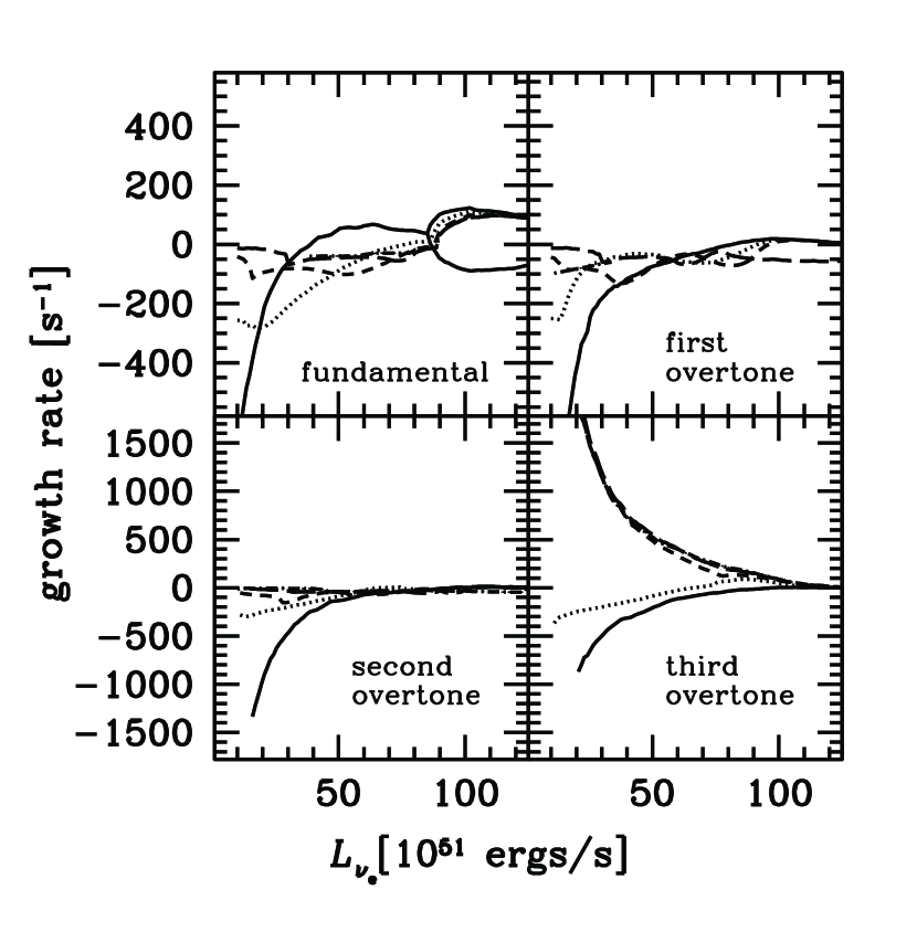
Figure 12: The growth rates, ${\rm Re}(\omega)$, of the non-radial modes with $\ell=1$ as a function of neutrino luminosity for different inner boundary radii. The fundamental mode (upper left panel), first overtone (lower left panel), second overtone (upper right panel), and third overtone (lower right panel) are shown. The solid, dotted dashed, long dashed and dash-dotted curves correspond to the result for the inner boundary radius of $1.0r_{\nu}$, $0.9r_{\nu}$, $0.8r_{\nu}$, $0.7r_{\nu}$, and $0.6r_{\nu}$, respectively. Notice that the vertical scales are different between the upper and lower panels.

which corresponds to the asymptotic expression for large $r$ of the original formula and is correct if neutrinos are propagating only radially. With this modification, we can extend the steady solution inwards continuously and smoothly although it is a very rough approximation to the actual situation inside the neutrino sphere. It should be mentioned, therefore, that the following models are of experimental nature and are not meant to be realistic. It is emphasized, however, that the treatment ensures no artificial generation of sound waves occurs at the neutrino sphere. Apart from this minor modification, we solved the same equations as given in §2 as well as in the previous paper (Yamasaki & Yamada, 2006), imposing the same condition, Eq. (27), at the shifted inner boundary. We can confirm that the results were little affected by the choice of the geometrical factor (compare the solid curve in the upper left pannel of Fig. 2 and that in Fig. 12).

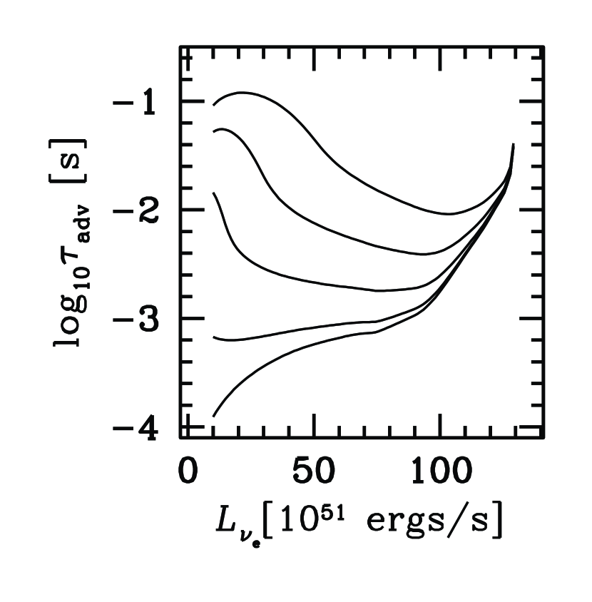
Figure 11: The advection time, ${\tau}_{\rm adv}$, in the region between shock and inner boundary. The radius of the inner boundary is altered. Each curve denotes the value for the case that the inner boundary is placed at $1.0r_{\nu}$, $0.9r_{\nu}$, $0.8r_{\nu}$, $0.7r_{\nu}$, $0.6r_{\nu}$ from bottom to top, respectively.

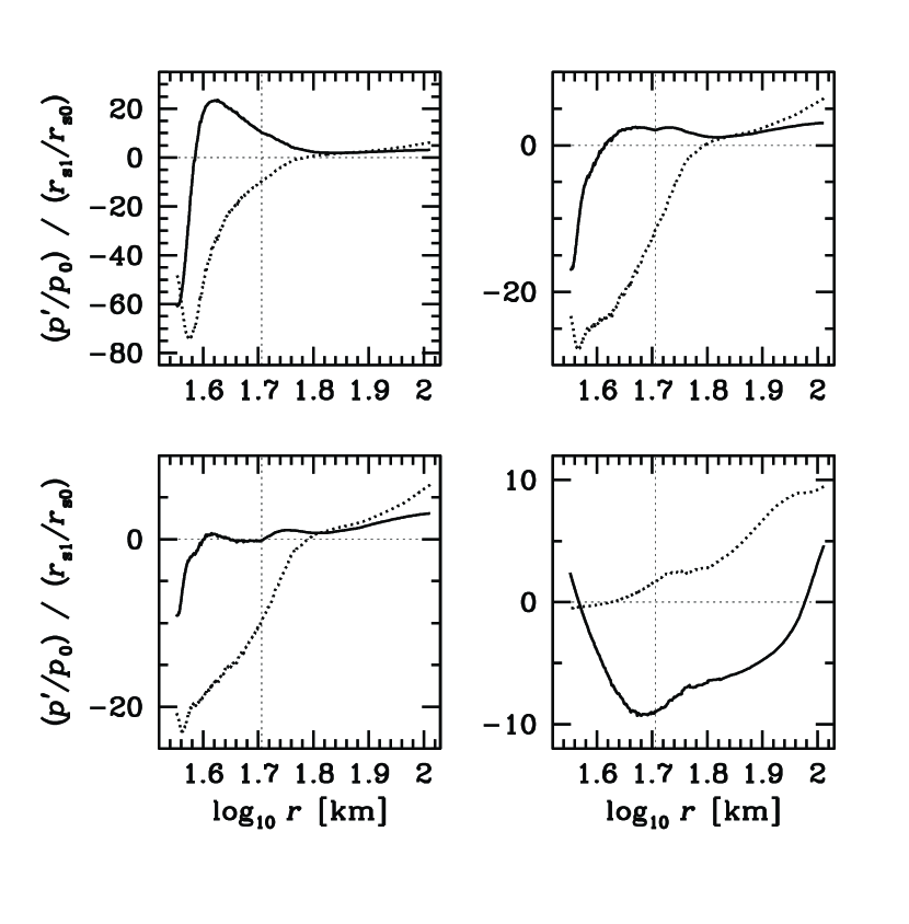
Figure 13: The eigen functions of the non-radial unstable mode with $\ell=1$ for $L_{\nu_{\rm e}}=6\cdot 10^{52}$ergs/s. The inner boundary is set at $r=0.7r_{\nu}$. The solid and dotted curves represent the real and imaginary parts, respectively. The fundamental mode (upper left panel), first overtone (upper right panel), second overtone (lower left panel), and third overtone (lower right panel) are shown. The vertical thin dotted lines represent the location of the neutrino sphere.

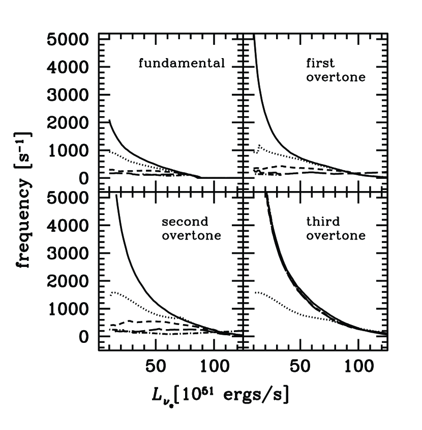
Figure 14: The oscillation frequencies, ${\rm Im}(\omega)$, of the non-radial modes with $\ell=1$ as a function of neutrino luminosity for different inner boundary radii. The fundamental mode (upper left panel), first overtone (upper right panel), second overtone (lower left panel), and third overtone (lower right panel) are shown. The solid, dotted, dashed, long dashed and dash-dotted curves correspond to the results for the inner boundary radius of $1.0r_{\nu}$, $0.9r_{\nu}$, $0.8r_{\nu}$, $0.7r_{\nu}$, and $0.6r_{\nu}$, respectively.

The results for the oscillatory modes are shown in Figs. 11 - 14. The advection time scales defined as

$$\tau_{\rm adv}\equiv-\int^{r_{\rm s}}_{r_{\rm in}}\frac{1}{u_{r}}dr,$$ (33)

are shown in Fig. 11. Here $r_{\rm in}$ is the radius of the inner boundary. As expected, the time scale is drastically increased as the location of the inner boundary is shifted more and more inwards. In Fig. 12, the growth rates of the modes with $\ell=1$ are given. We can see that the growth rates of the fundamental modes are remarkably reduced as the radius of the inner boundary gets smaller. We emphasize, however, that this does not imply that our previous results on the exsitence of the unstable modes were mere artefacts by the generation of sound waves at the inner boundary. Instead, what happened here is the change of characteristics of some eigen functions. In fact, as displayed in the upper left panel of Fig. 13, the perturbation amplitude for the fundamental mode in the present case becomes substantial only inside the neutrino sphere, which is qualitatively different from the correponding one given in the lower left panel of Fig. 5. As the radius of the inner boundary gets smaller, the sound waves generated deep inside the gravitational well are quickly damped as they propagate outwards. As a result, the vortex-acoustic cycle is not excited by these pressure waves. This is also the case for the first and second overtone modes as demonstrated in the upper right and lower left panels of the figure.

Sound waves are produced everywhere, though. It should be noted that higher overtones put more weight on the sound waves generated at larger radii, where they are not so severely damped. As a result, the vortex-acoustic cycle is excited not for the fundamental modes but for some higher overtones in the present case. This is demonstrated in the lower right panel of Fig. 12, where the third overtone is shown to be unstable. The eigen function for this mode is displayed in the lower right panel of Fig. 13, in which one can easily recognize its qualitative difference from the others. In Fig. 14, the oscillation frequencies of the modes with $\ell=1$ are given for different inner boundary radii. We can see that the oscillation frequencies of the unstable third overtone for $r_{\rm in}<0.8r_{\nu}$ are almost unchanged and close to $\tau_{\rm aa}$ but different from $\tau_{\rm pa}$. (It is noted that the $\tau_{\rm pa}$ is only slightly altered from those shown in Fig. 4 by shifting the radius of the inner boundary because the dislocation is much smaller than the distance between the shock and neutrino sphere and the sound velocity is larger inside the neutrino sphere than outside.) Hence the unstable third overtones appear to be excited by the vortex-acoustic couplings rather than by the purely acoustic cycles. Moreover, since the growth times of these unstable modes are much shorter than the advection time, the instabilities should be hardly affected by the production of sound waves at the inner boundary. They are indeed driven by the pressure perturbations generated near the neutrino sphere. On the other hand, the comparison between the growth rates of these modes and that of the fundamental mode obtained in §4 suggests that the solid boundary condition imposed at the neutrino sphere tended to suppress the excitation of the vortex-acoustic cycles. To summarize the effect of the shifted inner boundary on the oscillatory modes, the fundamental modes and some lower overtones are confined inside the neutrino sphere whereas higher overtones take over the roles that the fundamental and lower overtone modes have played in the previous models.

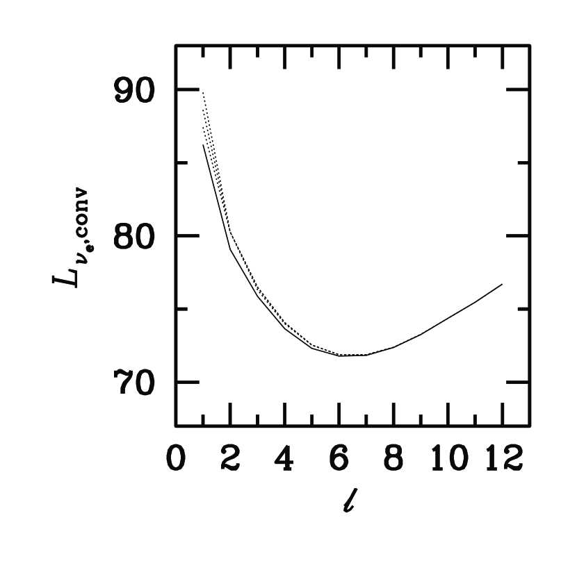
Figure 15: The same as the right bottom panel of Fig. 10 but for various values of the inner boundary radius. The solid curve corresponds to the inner boundary radius of $r=1.0r_{\nu}$. The dotted curves represent the results for the inner boundary radius of $r=0.9$, $0.8$, $0.7$, and $0.6r_{\nu}$ from bottom to top, respectively.

On the other hand, the growth of non-oscillatory modes is only slightly affected by the inward shift of the inner boundary (see Fig. 15). This is simply because the fluctuations for these modes grow mainly at a distant region from the neutrino sphere and the effects of over-generation of sound waves at the inner boundary, if any, are negligible for the unstable region. Therefore, the quantitative, but not qualitative, discrepancy between the results of Foglizzo et al. (2006a) and ours on the stability criterion for convection should be attributed to the difference in the treatment of the excitation of pressure perturbations between the gain radius and the neutrino sphere. The more complex background model we employed here may have also contributed somewhat to the difference.

We have observed that the solid boundary condition imposed at the neutrino sphere tends to stabilize the oscilatory modes and has essentially no influence on the non-oscilatory modes. The validity of the solid boundary condition itself is a remaining problem, though. This is a difficult issue, which could not be addressed based on the steady-state approximation, and the complete answer will be beyond the scope of this paper. In order to estimate the effect of different boundary conditions, however, we here adopt another conceivable condition, that is, the free boundary condition given by

$$\frac{du^{\prime}_{r}}{dr}=0$$ (34)

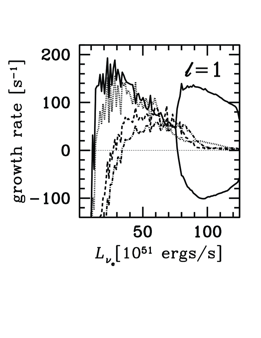
Figure 19: The growth rates, ${\rm Re}(\omega)$, for $\ell=1$ modes as a function of neutrino luminosity. The ”free” inner boundary condition was imposed for the radial-velocity perturbation. The solid curve represents the fundamental mode while the dotted, dashed and dash-dotted curves correspond to the first, second and third overtones, respectively.

at the inner boundary. This made the calculation of the linear perturbations much more difficult, however. In fact, we often came across the difficulty in obtaining a sufficient convergence of iterative calculations. As a result, the eigen values that we present below have much larger numerical errors systematically, which will be inferred from the artificial fluctuations in Fig. 19. In spite of the problem, we still think that we can obtain a result that is qualitatively correct and will be helpful for the society.

In Fig. 19, we plotted the growth rates, ${\rm Re}(\omega)$, for the $\ell=1$ modes as a function of the neutrino luminosity. This should be compared with the upper left panel of Fig. 2. The qualitative behavior of the fundamental mode is similar. However, the growth rate of unstable oscillation is a bit larger and the neutrino luminosity, at which the mode becomes unstable, is a little lower than in the model with the solid boundary condition. This seems to imply that the free inner boundary condition tends to enhance the instability, contrary to the naive expectation. This is also reflected in the behaviors of the overtones. In fact, while in the solid boundary case the overtone modes are almost stable up to the critical luminosity, in the free boundary case they are as unstable as the fundamental modes for relatively small luminosities. These results with the free boundary indicate that the qualitative results of the existence of the growing modes are not altered if the condition is significantly altered and suggest that the similar conclusion is expected if more reasonable condition, if it exists, is imposed.

Next we consider the variation of the perturbations of neutrino luminosity. In the previous sections, we assumed that the neutrino temperature (and luminosity, as a result) was not affected by the perturbations. This is based on the idea that neutrino luminosity is dominated by the contribution from the proto neutron star, which is little affected by the fluctuations of accretion flows. It is noted that the neutrino temperature characterizing its spectrum does not coincide in general with the matter temperature at the neutrino sphere. It is possible, however, that the neutrino emission from the accreted matter is more important and the fluctuation of the neutrino luminosity is correlated with the perturbation of matter temperature. Here we consider this case by imposing the condition that the variation of the neutrino temperature is proportional to that of the matter temperature, that is,

$$\left.\frac{T_{\nu 1}}{T_{\nu 0}}=\frac{T_{1}}{T_{0}}\right|_{r=r_{\nu}}.$$ (35)

We assumed that the temperature fluctuations given by Eq. (35) affect only the heating of the matter with the same polar and azimuthal angle ($\theta$, $\phi$).

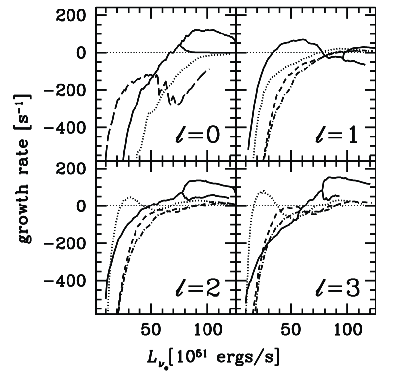
Figure 16: The growth rates, ${\rm Re}(\omega)$, for the radial, $\ell=0$, and non-radial modes, $\ell=1,2,3$, as a function of neutrino luminosity. The perturbation of neutrino temperature is taken into account. In the upper left panel, the solid curve represents the fundamental mode and the dotted curve presents the first overtone. The long dashed curve corresponds to the thermal mode. In the other panels, the solid curves represent the fundamental modes while the dotted, dashed and dash-dotted curves correspond to the first, second and third overtones, respectively.

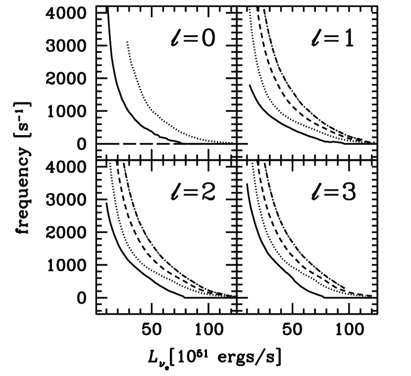
Figure 17: The oscillation frequencies, ${\rm Im}(\omega)$, for the radial, $\ell=0$, and non-radial modes, $\ell=1,2,3$, as a function of neutrino luminosity. The perturbation of neutrino temperature is taken into account. In the upper left panel, the solid curve represents the fundamental mode and the dotted curve presents the first overtone. The long dashed curve corresponds to the thermal mode. In the other panels, the solid curves represent the fundamental modes while the dotted, dashed and dash-dotted curves correspond to the first, second and third overtones, respectively.

The results are shown in Figs. 16 and 17. We show the growth rates and oscillation frequencies for the modes with $\ell=0-3$. Compared with the corresponding results shown in Figs. 2 and 3, the qualitative feature is unchanged. The thermal mode exists among the radial modes and is stable for all the neutrino luminosities as in the previous case. The first overtones of $\ell=2,3$ modes become unstable for relatively small luminosities. Then the fundamental $\ell=1$ mode takes over. They are all oscillatory. Again above $L_{\nu_{e}}\sim 7\times 10^{52}$ergs/s the fundamental modes are bifurcated into two branches and become non-oscillatory. Quantitatively, the growth rate is slightly modified with no clear tendency. The temporal variation of neutrino temperature sometimes helps the growth of the perturbations but other times not. It is determined by the integral of the fluctuations of heating over the entire cycle of the oscillation of the neutrino temperature. If the fluctuation of neutrino temperature and those of other quantities are synchronized, the perturbation is enhanced and vice versa. It should be also noted that the variation of the neutrino temperature is not necessarily synchronized with the temperature of the accreting matter at the neutrino sphere in reality.

We tried yet another case concerning the perturbation of neutrino emissions. For both cases considered thus far, the thermal mode was stable even at the critical luminosity, contraty to the results of the previous paper (Yamasaki & Yamada, 2005) (see the long dashed lines for the $\ell=0$ modes in Figs. 1 and 16). Although there are several differences between the previous and current papers, the inner boundary condition is likely to be the most important. Hence we took into account here the variation of the inner boundary radius in such a way that the density-perturbation be zero at the inner boundary for the perturbed flows. This is exactly the same treatment we adopted in the previous paper (Yamasaki & Yamada, 2005). Note that this condition is difficult to impose for non-radial modes, and we consider only the radial modes here.

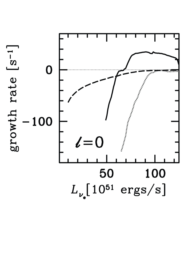
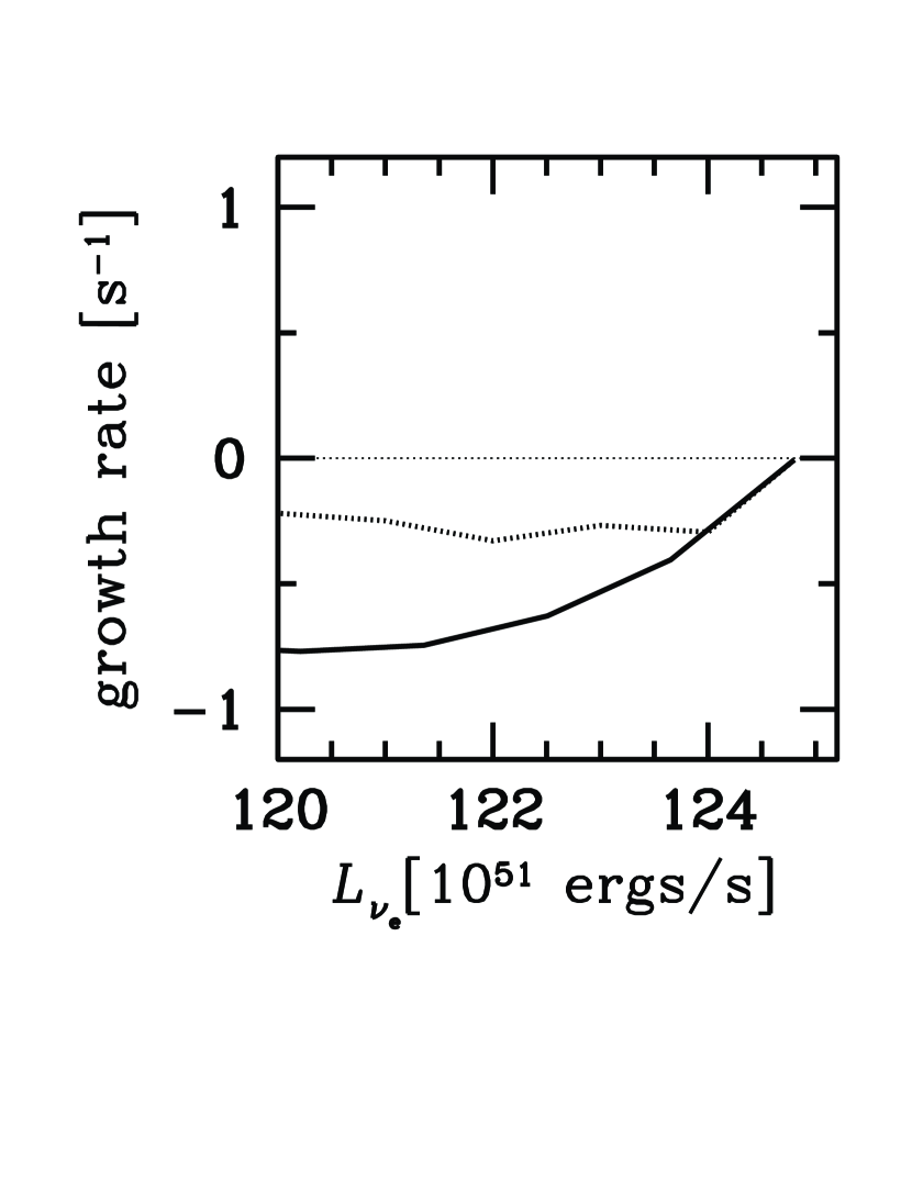
Figure 18: Left: The growth rates, ${\rm Re}(\omega)$ for representative radial ($\ell=0$) modes as a function of neutrino luminosity. The perturbations of neutrino temperature and neurtrino sphere are taken into account. The long dashed curve denotes the fundamental thermal mode. The solid and dotted curves correspond to the fundamental and first overtone oscillatory modes, respectively. Right: The same as in the left panel, but only those for the thermal modes both for the inner solution (solid curve) and the outer solution (dotted curve) are shown.

The results are shown in Fig. 18. The thermal mode denoted by the long dashed curve is stable below the crtical luminosity and becomes neutral at the critical point. The right pannel of the Fig. 18 is a zoom in to the critical point, and not only the inner solution but also the outer solution is displayed. They coincide with each other as a neutral mode at the critical luminosity. An interesting thing is that the outer solutions are also stable below the critical luminosity, contrary to the previous results by Yamasaki & Yamada (2005). It is noted, however, that the spherical accretion flows become unstable against the non-radial perturbations anyway. Another new feature is that the oscillatory radial fundamental mode (the solid curve in the left panel of Fig. 18) is not bifurcated up to the critical luminosity. The temporal variations of the neutrino sphere somehow delayed the occurence of the bifurcation. For the moment, we do not have a good explanation for this phenomenon. We do not know either whether other non-radial fundamental modes are also affected or not.

6 Summary and Discussions

In this paper, we investigated the stability of the spherically symmetric accretion flow through the standing shock wave onto the proto neutron star, which is supposed to approximate the post-bounce situation in the core-collapse supernova. We performed systematically the global linear-stability analyses for both radial and non-radial perturbations. We found that the flow is stable for all modes if the neutrino luminosity is lower than $\sim 1\times 10^{52}$ ergs/s in our models with $\dot{M}=1.0M_{\odot}/{\rm s}$. For larger luminosities, the non-radial instabilities are induced, probably via the advection-acoustic cycles. The modes with $\ell=2$ and $3$ become unstable at first for relatively low neutrino luminosities, e.g. $\sim 2-3\times 10^{52}$ ergs/s for the same accretion rate, whereas the $\ell=1$ mode is the most unstable for higher luminosities, $\sim 3-7\times 10^{52}$ ergs/s. These are all oscillatory modes. For still higher luminosities, $\gtrsim 7\times 10^{52}$ ergs/s, the non-oscillatory modes become unstable, among which we identified the non-radial ones as convection. In this way, we discussed the convective instability in the presence of advection on the same basis. We found that the growth rates of the convective modes change gradually with $\ell$ and have a peak at $\ell=5-11$, depending on the luminosity. The luminosity, at which each convective mode becomes unstable, decreases with $\ell$ up to $\ell=6$ and then increases for the same accretion rate. We confirmed the results obtained by numerical simulations that the instabilities induced by the advection-acoustic cycles become more important than convections for lower neutrino luminosities. We modified the criterion for the convection in the presence of advection previously discussed by Foglizzo et al. (2006a). Furthermore, we investigated the sensitivity of the results to the inner boundary conditions and found that the nature of the instabilities is not changed qualitatively.

In most of realistic simulations, the neutrino luminosity seems to be much smaller than the critical value (see e.g. (Janka et al., 2005; Sumiyoshi et al., 2005)). Hence, from the results of this paper, the over-stabilizing modes induced probably by the advection-acoustic cycles are more important than convections in causing the global anisotropy as observed in the ejecta of core-collapse supernovae (Leonard et al., 2000; Wang et al., 2002). The instability is normally saturated at some amplitudes owing to the non-linear coupling of various modes (Ohnishi et al., 2006a). Although the instability of the standing shock wave, whatever the cause, is helpful for the shock revival, recent multi-dimensional numerical simulations (Janka et al., 2005) demonstrated that these instabilities alone could not induce an explosion. Then there must be some other agents to further boost the shock revival. Very recently Burrows et al. (2006) proposed a new mechanism, in which the dissipation of out-going acoustic waves that are excited by g-mode oscillations in the proto neutron star is the agent of the shock revival. In this context, the possible coupling between the instabilities of the accretion flows and the oscillations of the proto neutron star are interesting (Yoshida et al., 2006; Ohnishi et al., 2006b).

In this paper, we considered only the spherically symmetric background flows. Considering the fact that massive stars are rotating in general, we are naturally concerned with the stability of rotational accretion flows. In the previous paper (Yamasaki & Yamada, 2005), we showed that the rapid rotation changes steady accretion flows in such a way that the critical luminosity is decreased and, as a result, the shock revival is facilitated. In so doing, we found that some of the models have a negative entropy gradient and can be convectively unstable. ¿From the results of this paper, we also expect some oscillatory modes will become unstable and will be more important than convection for low neutrino luminosities. Magnetic fields may also play an important role for the stability of accretion flows. Then, the so-called magneto-rotational instability (MRI) should be discussed in the same framework. In the case of the spherically symmetric background considered in this paper, each eigen value is degenerate with respect to the index, $m$. In the presence of rotation and/or magnetic field, the degeneracy will be removed at least partially. Furthermore, how the growth rates themselves are modified by these effects is an interesting issue. We are currently undertaking the task (Yamasaki & Yamada, 2006b) and the results will be published elsewhere.

Appendix A Heating and Reaction Rates

As for the neutrino reactions, we take into account only the dominant contributions: the emission and absorption by free nucleons.

$$p+e^{-}\rightleftharpoons\nu_{e}+n,$$ (A1)

$$n+e^{+}\rightleftharpoons\bar{\nu}_{e}+p.$$ (A2)

Then the heating and reaction rates can be decomposed as

$$\dot{q}=\dot{q}_{\rm ep}-\dot{q}_{\nu{\rm n}}+\dot{q}_{\rm e^{+}n}-\dot{q}_{\bar{\nu}{\rm p}},$$ (A3)

$$\lambda=-\lambda_{\rm ep}+\lambda_{\nu{\rm n}}+\lambda_{\rm e^{+}n}-\lambda_{\bar{\nu}{\rm p}},$$ (A4)

and are calculated based on the formulae given by Bruenn (1985) as follows.

The absorption and emission kernels for the source terms in the Boltzmann equation are given as

$$R^{a}_{1}=\frac{1}{\hbar^{7}c^{7}}\frac{G_{\rm F}^{2}}{\pi}\eta_{np}(3g_{A}^{2}+g_{V}^{2})\{1-F_{e}(E+\Delta)\}(E+\Delta)^{2}\sqrt{1-\frac{m_{e}^{2}c^{4}}{(E+\Delta)^{2}}},$$ (A5)

$$R^{e}_{1}=\exp\{-\beta(E-\mu_{p}-\mu_{e}+\mu_{n})\}\cdot R^{a}_{1},$$ (A6)

where the following notations are used:

$$\eta_{np}=C\int\frac{2d^{3}p}{(2\pi\hbar c)^{3}}F_{n}(E)\cdot(1-F_{p}(E)),$$ (A7)

$$\Delta=(m_{n}-m_{p})c^{2}.$$ (A8)

The mass and chemical potential of the particle of type $i$ are denoted as $m_{i}$, $\mu_{i}$, respectively; $\beta=1/kT$ ($k$ is the Boltzmann constant) is the inverse temperature and $E=p^{2}/2m_{i}$ is the kinetic energy of each particle; $\hbar$, $c$, $G_{\rm F}$ are the Planck constant, speed of light and Fermi coupling constant, respectively; the unit is chosen such a way that $G_{\rm F}/(\hbar c)^{3}=1.166\cdot 10^{-11}[{\rm MeV}^{-2}]$, and we adopt the values of form factors as $g_{V}=1$, $g_{A}=1.23$; $F_{i}(E)$ is the distribution function for the particle of type $i$ and is assumed be the Fermi-Dirac distribution:

$$F_{i}(E)=\frac{1}{1+\exp\{\beta(E-\mu_{i})\}}.$$ (A9)

In Eq. (A7) we have introduced the factor

$$C=\frac{\displaystyle{n_{n}}}{\displaystyle{\frac{2}{(2\pi\hbar)^{3}}\int F_{n}(E)d^{3}p}},$$ (A10)

which takes account of the discrepancy between the realistic EOS for nucleons we employ in the calculations and the ideal-gas EOS assumed in the above formulae. $n_{n}$ is the number density of neutron given by the realistic EOS.

Considering the fact that the region of our interest is optically thin for neutrinos, that is, outside the neutrino sphere, we can write the heating and reaction rates, $\dot{q}_{ep}$, $\dot{q}_{\nu n}$, $\lambda_{ep}$ and $\lambda_{\nu n}$, as

$$\dot{q}_{ep}=\frac{4\pi c}{(2\pi\hbar c)^{3}}\int R^{e}_{1}\{1-fF_{\nu}(E)\}E^{3}dE,$$ (A11)

$$\dot{q}_{\nu n}=\frac{4\pi c}{(2\pi\hbar c)^{3}}\int R^{a}_{1}fF_{\nu}(E)E^{3}dE,$$ (A12)

$$\lambda_{ep}=\frac{4\pi c}{(2\pi\hbar c)^{3}}\int R^{e}_{1}\{1-fF_{\nu}(E)\}E^{2}dE,$$ (A13)

$$\lambda_{\nu n}=\frac{4\pi c}{(2\pi\hbar c)^{3}}\int R^{a}_{1}fF_{\nu}(E)E^{2}dE,$$ (A14)

where $fF_{\nu}(E)$ is the local distribution function of irradiating neutrinos. We take the Fermi-Dirac distribution with a temperature $T_{\nu}$ and a vanishing chemical potential for$F_{\nu}(E)$:

$$F_{\nu}(E)=\frac{1}{1+\exp(E/kT_{\nu})},$$ (A15)

whereas $f$ is the so-called geometrical factor, which takes account of the fraction of solid angle that the neutrinos emitted from the neutrino sphere occupy at each point:

$$f=\frac{1-\sqrt{1-(r_{\nu}/r)^{2}}}{2}.$$ (A16)

In a similar way, the absorption and emission kernels for the reaction given by Eq. (A2) can be written as,

$$R^{a}_{2}=\frac{1}{\hbar^{7}c^{7}}\frac{G_{\rm F}^{2}}{\pi}\eta_{pn}(3g_{A}^{2}+g_{V}^{2})\{1-F_{e^{+}}(E-\Delta)\}(E-\Delta)^{2}\sqrt{1-\frac{m_{e}^{2}c^{4}}{(E-\Delta)^{2}}}\Theta(E-\Delta-m_{e}c^{2}),$$ (A17)

$$R^{e}_{2}=\exp\{-\beta(E-\mu_{n}-\mu_{e^{+}}+\mu_{p})\}\cdot R^{a}_{2},$$ (A18)

where we use the following notations:

$$\eta_{pn}=C\int\frac{2d^{3}p}{(2\pi\hbar c)^{3}}F_{p}(E)\cdot(1-F_{n}(E)),$$ (A19)

$$\Theta(x)=\left\{\begin{array}[]{rl}1,&\qquad\mbox{for $x\geq 0$}\\ 0,&\qquad\mbox{for $x<0$}.\end{array}\right.$$ (A20)

Then the heating and reaction rates, $\dot{q}_{e^{+}n}$, $\dot{q}_{\bar{\nu}p}$, $\lambda_{e^{+}n}$ and $\lambda_{\bar{\nu}p}$, are given as

$$\dot{q}_{e^{+}n}=\frac{4\pi c}{(2\pi\hbar c)^{3}}\int R^{e}_{2}\{1-fF_{\bar{\nu}}(E)\}E^{3}dE,$$ (A21)

$$\dot{q}_{\bar{\nu}p}=\frac{4\pi c}{(2\pi\hbar c)^{3}}\int R^{a}_{2}fF_{\bar{\nu}}(E)E^{3}dE,$$ (A22)

$$\lambda_{e^{+}n}=\frac{4\pi c}{(2\pi\hbar c)^{3}}\int R^{e}_{2}\{1-fF_{\bar{\nu}}(E)\}E^{2}dE,$$ (A23)

$$\lambda_{\bar{\nu}p}=\frac{4\pi c}{(2\pi\hbar c)^{3}}\int R^{a}_{2}fF_{\bar{\nu}}(E)E^{2}dE,$$ (A24)

where $fF_{\bar{\nu}}(E)$ is the local distribution function of irradiating anti-neutrinos with $F_{\bar{\nu}}(E)$ being the Fermi-Dirac distribution function with a temperature $T_{\nu}$ and a vanishing chemical potential just like in Eq. (A16) and $f$ being the geometrical factor.

References

- Blondin et al. (2003) Blondin, J. M., Mezzacappa, A., & DeMarino, C. 2003, ApJ, 584, 971
- Blondin & Mezzacappa (2006) Blondin, J. M., & Mezzacappa, A. 2006, ApJ, 642, 401
- Bruenn (1985) Bruenn, A. 1985, ApJS, 58, 771
- Burrows & Goshy (1993) Burrows, A., & Goshy, J. 1993, ApJ, 416, L75
- Burrows et al. (2006) Burrows, A., Livne, E., Dessart, L., Ott, C.D., & Murphy, J. 2006, ApJ, 640, 878
- Foglizzo & Tagger (2000) Foglizzo, T., & Tagger, M. 2000, A&A, 363, 174
- Foglizzo (2001) Foglizzo, T. 2001, A&A, 368, 311
- Foglizzo (2002) Foglizzo, T. 2002, A&A, 392, 353
- Foglizzo & Galletti (2004) Foglizzo, T., & Galletti, P. 2004, Cosmic explosions in three dimensions : asymmetries in supernovae and gamma-ray bursts. Cambridge contemporary astrophysics series. Cambridge University Press, 2004, p.238
- Foglizzo et al. (2005) Foglizzo, T., Galletti, P., & Ruffert, M. 2005, A&A, 435, 397
- Foglizzo et al. (2006a) Foglizzo, T., Scheck, L., & Janka, H.-Th. 2006a, ApJ, in press, (astro-ph/0507636)
- Foglizzo et al. (2006b) Foglizzo, T., Galletti, P., Scheck, L., & Janka, H.-Th. 2006b, ApJ, in press, (astro-ph/0606640)
- Galletti & Foglizzo (2005) Galletti, P., & Foglizzo, T. 2005, EdP-Sciences, Conference Series, 2005, p. 487
- Heger et al. (2000) Heger, A., Langer, N., & Woosley, S. E. 2000, ApJ, 528, 368
- Heger et al. (2004) Heger A, Woosley S. E., Langer N., & Spruit H. C. 2004 Proc. IAU 215 Stellar Rotation, p. 591
- Houck & Chevalier (1992) Houck, J. C., & Chevalier, R. A. 1992, ApJ, 395, 592
- Howe (1975) Howe, M. S. 1975, J. Fluid Mech., 71, 625
- Janka et al. (2005) Janka, H. -Th., Buras, R., Kitaura Joyanes, F. S., Marek, A., Rampp, M. & Scheck, L. 2005, NPA, 758, 19
- Kotake et al. (2006) Kotake, K., Sato, K., & Takahashi, K. 2006, Rept.Prog.Phys. 69, 971-1144
- Leonard et al. (2000) Leonard, D. C., Filippenko, A. V., Barth, A. J., & Matheson, T. 2000, ApJ, 536, 239
- Liebendörfer et al. (2005) Liebendörfer, M., Pen, U., & Thompson, C. 2005, Nucl. Phys., A758, 59
- Lyne & Lorimer (1994) Lyne, A. G., & Lorimer, D. R., 1994, Nature, 369, 127
- Nakayama (1992) Nakayama, K. 1992, MNRAS, 259, 259
- Nakayama (1993) Nakayama, K. 1993, PASJ, 45, 167
- Nakayama (1994) Nakayama, K. 1994, MNRAS, 270, 871
- Ohnishi et al. (2006a) Ohnishi, N., Kotake K., & Yamada, S. 2006a, ApJ, 641, 1018
- Ohnishi et al. (2006b) Ohnishi, N., Kotake K., & Yamada, S. 2006b, in preparation
- Scheck et al. (2004) Scheck, L., Plewa, T., Janka, H.-Th., Kifonides, K., & Müller, E. 2004, Phys. Rev. Lett., 92, 011103
- Shen et al. (1998) Shen, H., Toki, H., Oyamatsu, K., & Sumiyoshi, K. 1998, Nucl. Phys. A, 637, 435
- Sumiyoshi et al. (2005) Sumiyoshi, K., Yamada, S., Suzuki, S., Shen, H., Chiba, S.,& Toki, H. 2005, ApJ, 629, 922
- Wang et al. (2002) Wang, L., Wheeler, J. C., Höflich, P., Khokhlov, A., Baade, D., Branch, D., Challis, P., Filippenko, A. V., Fransson, C., Garnavich, P., Kirshner, R. P., Lundqvist, P., McRay, R., Panagia, N., Pun, C. S. J., Phillips, M. M., Sonneborn, G., & Suntzeff, N. B. 2002, ApJ, 579, 671
- Yamasaki & Yamada (2005) Yamasaki, T., & Yamada, S. 2005, ApJ, 623,1000
- Yamasaki & Yamada (2006) Yamasaki, T., & Yamada, S. 2006, ApJ, in press, (astro-ph/0606504)
- Yamasaki & Yamada (2006b) Yamasaki, T., & Yamada, S. 2006, in preparation
- Yoshida et al. (2006) Yoshida, S., Ohnishi, N., & Yamada, S. 2006b, in preparation