GaBoDS: The Garching-Bonn Deep Survey

Abstract

Aims. The clustering properties of a large sample of $U$-dropouts are investigated and compared to very precise results for $B$-dropouts from other studies to identify a possible evolution from $z=4$ to $z=3$.

Methods. A population of $\sim 8800$ candidates for star-forming galaxies at $z=3$ is selected via the well-known Lyman-break technique from a large optical multicolour survey (the ESO Deep Public Survey). The selection efficiency, contamination rate, and redshift distribution of this population are investigated by means of extensive simulations. Photometric redshifts are estimated for every Lyman-break galaxy (LBG) candidate from its $UBVRI$ photometry yielding an empirical redshift distribution. The measured angular correlation function is deprojected and the resulting spatial correlation lengths and slopes of the correlation function of different subsamples are compared to previous studies.

Results. By fitting a simple power law to the correlation function we do not see an evolution in the correlation length and the slope from other studies at $z=4$ to our study at $z=3$. In particular, the dependence of the slope on UV-luminosity similar to that recently detected for a sample of $B$-dropouts is confirmed also for our $U$-dropouts. For the first time number statistics for $U$-dropouts are sufficient to clearly detect a departure from a pure power law on small scales down to $\sim 2\arcsec$ reported by other groups for $B$-dropouts.

1 Introduction

For more than a decade now, the high-redshift universe has become reachable by observations mainly due to the development of efficient colour selection techniques. The group around C. C. Steidel (Steidel & Hamilton 1993; Steidel et al. 1996, 1999) has introduced the Lyman-break technique selecting high-redshift, star-forming galaxies from optical multicolour data by their pronounced Lyman-break. Many groups have used this technique and analysed various properties of these galaxy populations from redshifts $z\approx 3$ up to $z\approx 7$.

A particular emphasis in these studies was given to the clustering properties of the Lyman-break galaxy (LBG) samples (Steidel et al. 1998; Giavalisco et al. 1998; Adelberger et al. 1998, 2005; Giavalisco & Dickinson 2001; Ouchi et al. 2001, 2004, 2005; Porciani & Giavalisco 2002; Bouché & Lowenthal 2004; Foucaud et al. 2003; Allen et al. 2005; Lee et al. 2006; Kashikawa et al. 2006; Gawiser et al. 2006). Going back in cosmic time the correlation strength of these high-$z$ galaxies can be directly compared to $N$-body simulations or semi-analytical predictions yielding estimates of, e.g., the galaxy bias for early epochs. These results can then be used as an input for models of galaxy formation, and help to constrain the large number of free parameters to adjust. The more precise our knowledge of the clustering evolution becomes the more accurate our understanding of galaxy evolution will be.

In this context it is of crucial importance to reach a similar precision for the same galaxy populations at different redshifts. While in the beginning most LBG studies concentrated on relatively bright $z=3$ $U$-dropouts, in the last years more and more groups have focused on the investigation of LBGs at redshifts around $z=4$ selected as $B$-dropouts. This is obviously due to the fact that deep and wide $U$-band images are still a very telescope-time consuming task and some recent wide-field cameras like Suprimecam or space-based surveys like GOODS even lack a $U$-filter entirely.

By estimating the angular correlation function of nearly 17 000 $B$-dropouts selected from the Subaru/XMM-Newton Deep Field, Ouchi et al. (2005) find evidence for a departure from a pure power law on small scales. The same trend is reported by Lee et al. (2006) for $B$- and $V$-dropouts from the very deep GOODS ACS data. Neither the number statistics in the former study mentioned nor the depth and angular resolution of the GOODS data have a comparable counterpart at slightly lower redshifts. The most precise estimates of $U$-dropout clustering to date come from Adelberger et al. (2005) estimating the angular correlation function but not reporting any obvious excess on small scales. The question whether this is an evolutionary effect or whether this feature is only visible in the $z=4$ data because of their superior quality can only be answered by a $U$-dropout survey comparable in size to the $B$-dropout surveys mentioned above.

In this paper we describe our investigations of $z=3$ LBGs in the ESO Deep Public Survey (DPS). The methods presented here are based on our investigations in the Chandra Deep Field South (the DPS field Deep2c) presented in Hildebrandt et al. (2005). In Sect. 2 the data of the DPS and the selection of the LBGs are described. Simulations to assess the performance of our LBG selection are presented in Sect. 3. The clustering analysis is covered in Sect. 4. A summary and conclusions are given in Sect. 5.

Throughout this paper we adopt a standard $\Lambda$CDM cosmology with $\left[H_{0},\Omega_{\mathrm{m}},\Omega_{\Lambda},\sigma_{8}\right]=\left[70\,\mathrm{km\,s^{-1}\,Mpc^{-1}},0.3,0.7,0.9\right]$. We use Vega magnitudes if not stated otherwise.

2 The data and the samples

2.1 DPS images

The ESO Deep Public Survey is a deep multicolour survey carried out with the Wide Field Imager (WFI), an eight-chip CCD camera of $34\arcmin\times 33\arcmin$ field-of-view mounted at the MPG/ESO2.2 m telescope at La Silla. The images used for this study are described in Hildebrandt et al. (2006) along with the characteristics of the WFI filter-set. Furthermore, details on the raw data, the data reduction with our THELI pipeline (Erben et al. 2005), the astrometric and photometric calibration, the quality control, and the data release to the scientific community can be found there.

For our studies on LBGs we use seven fields (2 sq. deg) with complete coverage in the $UBVRI$-filters, in particular the fields Deep1a, 1b, 2b, 2c, 3a, 3b, and 3c, respectively. Their properties are summarised in Table 1.

Table 1: The DPS fields with five colour coverage. The limiting magnitudes in columns four to eight are measured in a circular aperture of $2\times$FWHM diameter from the $1\sigma$ sky background fluctuations of the images before convolution with a Gaussian filter (see text). In column nine the seeing FWHM values after convolution are given. Column ten contains the number of objects satisfying Eq. (2.4). In the fields Deep2b and Deep3a less $U$-dropouts are selected due to inferior quality of the imaging data (see text). The completeness limits for LBG selection in column eleven are estimated from Fig. 2. These visual estimates are very rough with an accuracy of $\sim 0.5\,\mathrm{mag}$. The effective area used for LBG selection is given in the last column.

field	RA [h m s]	Dec [d m s]	1-$\sigma$ mag lim. [Vega mags]					conv.	$N_{\mathrm{LBG}}$	LBG compl. limit	eff. area
	J2000.0	J2000.0	$U$	$B$	$V$	$R$	$I$	seeing		$R$	[$\mathrm{arcmin}^{2}$]
Deep1a	22:55:00.0	$-$40:13:00	27.0	27.8	27.5	27.4	26.3	$1\aas@@fstack{\prime\prime}3$	1420	25.0	1045
Deep1b	22:52:07.1	$-$40:13:00	27.0	27.5	27.1	27.2	26.2	$1\aas@@fstack{\prime\prime}3$	1114	24.5	1036
Deep2b	03:34:58.2	$-$27:48:46	26.8	28.0	27.5	26.9	26.3	$1\aas@@fstack{\prime\prime}3$	492	24.0	1025
Deep2c	03:32:29.0	$-$27:48:46	27.1	29.0	28.6	28.5	26.3	$1\aas@@fstack{\prime\prime}0$	2181	25.5	1064
Deep3a	11:24:50.0	$-$21:42:00	26.6	27.9	27.2	27.3	25.8	$1\aas@@fstack{\prime\prime}1$	456	24.0	1033
Deep3b	11:22:27.9	$-$21:42:00	26.9	27.9	27.3	27.3	26.2	$1\aas@@fstack{\prime\prime}0$	1484	25.0	1072
Deep3c	11:20:05.9	$-$21:42:00	27.0	28.1	27.3	27.2	25.8	$1\aas@@fstack{\prime\prime}0$	1679	25.0	998
									$\Sigma=8826$		$\Sigma=7273$

Note that the images of the field Deep2c used in the current study are different from the images used in Hildebrandt et al. (2005). More data have become available so that the current images in this field are considerably deeper.

2.2 Catalogue extraction

First, the different colour images of one field are trimmed to the same size. The seeing is measured for these images and SExtractor (Bertin & Arnouts 1996) is used to create RMS maps. From these RMS images the local limiting magnitude ($1\sigma$ sky background in a circular aperture of $2\times$FWHM diameter) in each pixel is calculated and limiting magnitude maps are created. Then every image is convolved with an appropriate Gaussian filter to match the seeing of the image with the worst seeing value.

For the catalogue extraction SExtractor is run in dual-image mode with the unconvolved $R$-band image for source detection and the convolved images in the five bands for photometric flux measurements. In this way it is assured that the same part of a galaxy is measured in every band. In the absence of a strong spatial colour gradient in an object this method should lead to unbiased colours especially for high-redshift objects of small apparent size. In the following, we use isophotal magnitudes when estimating colours or photometric redshifts of objects. The total $R$-band magnitudes always refer to the SExtractor parameter MAG_AUTO measured on the unconvolved $R$-band image.

2.3 Photometric redshift estimation

Photometric redshifts are estimated for all objects in the catalogue from their $UBVRI$ photometry using the publicly available code Hyperz (Bolzonella et al. 2000). The technique applied is essentially the same as described in Hildebrandt et al. (2005) with the only difference that in the current study we use isophotal magnitudes extracted from images with matched seeing instead of seeing adapted aperture magnitudes. In Hildebrandt et al. (2006, in preparation) we compare our photometric redshift estimates to several hundred spectroscopic redshifts from the VIMOS VLT Deep Survey (VVDS; Le Fèvre et al. 2004) in the field Deep2c and find that the combination of isophotal magnitudes with the templates created from the library of Bruzual & Charlot (1993) yields the smallest scatter and outlier rates at least for the redshifts probed by the VVDS ($z<1.4$). For $R<24$ we find a standard deviation of $\sigma=0.052$ for the quantity $\Delta z=\left(z_{\mathrm{spec}}-z_{\mathrm{phot}}\right)/\left(1+z_{\mathrm{spec}}\right)$ after rejecting 5% of outliers (objects with $\Delta z>0.15$). With increasing redshift and decreasing angular size of the objects the isophotal magnitudes on images with matched seeing should approach the seeing adapted aperture magnitudes. Investigating the redshift distributions of our $U$-dropout sample (see below) we see no significant difference between the two approaches so that the results of the clustering measurements are not influenced by this choice.

2.4 Sample selection

In Hildebrandt et al. (2005) we chose quite conservative criteria for our $U$-dropout selection. In particular, we tried to define colour cuts in such a way to avoid regions in colour space with a considerable amount of contamination. Supported by our simulations (see Sect. 3), and after refining our photometric measurements (see above), which should yield better colours, especially for the possible contaminants, we decided to relax our selection criteria. The performance of our selection in terms of contamination and efficiency is analysed in Sect. 3 by means of simulated colour catalogues. In Fig. 1 the colour-colour diagram for one field is shown with the old and the new selection criteria represented by the boxes. We select candidates for $z=3$ LBGs in the following way:

$$0.3 < (U-V)\;,$$

$$-0.5 < (V-R)<1.5\;,$$ (1)

$$3(V-R) < (U-V)+0.2\;,$$

Figure 1: $(U-V)$ vs. $(V-R)$ colour-colour diagram of galaxies in the field Deep2c. The upper box represents the old selection criteria adopted in Hildebrandt et al. (2005) while the lower extension represents the selection criteria of the current study. The $(U-V)$ colours of objects that are satisfying the LBG selection criterea but are not detected in the $U$-band are lower limits (arrows). In contrast the detected objects satisfying the selection criterea are plotted as filled circles.

Furthermore, we require every candidate to be detected in $V$ and $R$ and to be located in a region on our images where the local limiting magnitudes in $UVR$ are not considerably decreased. This is necessary to avoid complex selection effects in colour space due to varying depths over a single field. In our catalogues we find 8826 objects satisfying these selection criteria.

Every candidate is inspected visually in all five filters. Moreover, the redshift-probability distribution (see Hildebrandt et al. 2005), the location in the field, and the location in the colour-colour diagram is checked for every object. Approximately one third of the candidates is rejected in this way. Most of these rejected objects are influenced by the straylight from bright neighbouring objects (indicated by their extraction flags or visible in the $10^{\prime\prime}\times 10^{\prime\prime}$ thumbnail images) so that their colours cannot be trusted. Merely 72 objects ($<1\%$) are rejected due to their redshift-probability distribution in combination with a suspicious location in the colour-colour diagram near the stellar locus. Thus, the photometric redshift distribution is almost not affected by the exclusion of these objects.

The magnitude dependent angular number-densities of the accepted candidates for the seven fields and for the whole DPS are displayed in Fig. 2 in comparison to the values found by Steidel et al. (1999). For $R<24$ all seven fields show approximately the same LBG source density within a reasonable field-to-field variance. The field Deep2b can be regarded as fairly complete down to $R=24.5$ and the fields Deep1a, 3b, and 3c, respectively, down to $R=25$. But only the field Deep2c shows the same density as the survey by Steidel et al. (1999) down to $R=25.5$. The underdensity of Deep1b and Deep2b can be explained by the inferior seeing in the detection images ($R$) while the underdensity of Deep3a is due to a shallower $U$-band image.

Figure 2: Source counts of LBGs as a function of $R$-band magnitude. The DPS densities are represented by crosses while the Steidel et al. (1999) densities are represented by triangles which are offset by +0.1 mag just for clarity.

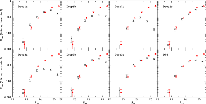
As long as one restricts investigations in a given magnitude bin to fields that can be regarded as uniform in terms of LBG selection, these investigations are not subject to systematic effects due to varying selection efficiency between the fields. This is in particular important in the clustering analysis to avoid artificial correlations originating from non-uniform depths.

The photometric redshift distribution of all accepted objects is shown in Fig. 3. The mean redshift of $\left<z\right>=2.96$ (4-$\sigma$ outliers are rejected) is essentially the same as the spectroscopic mean found by Adelberger et al. (2005) for their LBG sample, but our distribution seems to be slightly narrower ($\sigma=0.24$). However, without spectroscopic information we are not able to judge whether this is due to the different selection method with a different camera and filter set or due to imperfect photometric redshift estimation. In the following we will use the distribution inferred from our photometric redshifts indicating whenever the width has a large influence on our results.

Figure 3: Photometric redshift distribution of all accepted LBG candidates. The distribution has a mean of $\left<z\right>=2.96$ and an RMS of $\sigma=0.24$.

3 Simulations of objects’ colours in the DPS

Without a large spectroscopic survey of our LBGs at hand the only possible way to estimate properties of our LBG samples like, e.g., the contamination rate is to create a simulated colour catalogue.

3.1 The role of stars in our sample

The TRILEGAL galactic model by Girardi et al. (2005) is used to simulate the number of stars in all seven fields and their colours in the WFI filter set. In this way we obtain accurate $U-V$ and $V-R$ colours and are able to quantify the amount of stellar contamination in the LBG selection box. In Fig. 4 the colours of stars in the field Deep1a are shown, representative for the whole survey. The selection criteria were chosen in such a way that stellar contamination is very low, which is confirmed by Fig. 4 (see also the bottom panel of Fig. 10).

Figure 4: $(U-V)$ vs. $(V-R)$ colour-colour diagram of simulated stars in the field Deep1a. The boxes are the same as in Fig. 1.

3.2 Colours of galaxies

The code Hyperz cannot only be used to estimate photometric redshifts but also to create colour catalogues of galaxies at different redshifts and of different spectral types. We simulate huge random mock catalogues in magnitude bins of width 0.5 mag of 500 000 galaxies each, evenly distributed over the redshift interval $0<z<7$ and over all spectral types from the library of Bruzual & Charlot (1993) provided by Hyperz. Magnitude errors are simulated by Hyperz according to the 1-$\sigma$ limits in the five bands. This is done separately for every field taking into account the different depths in the five bands. From the photometric redshift code BPZ (Benítez 2000) we extract magnitude- and spectral type-dependent redshift distributions derived from the Hubble Deep Field. We assign the two reddest Hyperz spectral types from the library of Bruzual & Charlot (1993) (“Burst” and “E”) to the BPZ $z$-distribution for elliptical galaxies, two intermediate types (“Sb” and “Sc”) to the $z$-distribution for spirals, and the two bluest spectral types (“Sd” and “Im”) to the $z$-distribution for star-forming galaxies. Galaxies are taken from the evenly distributed catalogues with numbers and spectral types according to these redshift distributions to create realistic catalogues for 0.5 mag intervals. Finally, from these catalogues the galaxies are taken with numbers scaled to the $I$-band number-counts in the seven fields. In this way, for every field a catalogue is created which gives a fair representation of our data in 0.5 mag wide intervals. The $U-V$ vs. $V-R$ colour-colour diagram of the simulated galaxies is shown in Fig. 5.

Certainly, it is a strong assumption that the chosen template set represents the galaxy population in our data at all redshifts. Furthermore, the redshift distributions were extracted from the Hubble Deep Field which is subject to cosmic variance. These shortcomings are most probably responsible for the slight differences between Fig. 1 and Fig. 5 and the simulations should only be regarded as rough estimates.

Figure 5: $(U-V)$ vs. $(V-R)$ colour-colour diagram of simulated galaxies. The boxes are the same as in Fig. 1. Objects with a redshift of $z>2.5$ are plotted as crosses. We find good agreement in the overall shape of the colour distribution of the simulated galaxies to the real data (see Fig. 1). The slight differences, however, may be attributed to an imperfect template set and to a redshift distribution which is subject to cosmic variance.

Applying the colour cuts from Eq. (2.4) to the simulated star- and galaxy-catalogues we obtain estimates for the contamination rate in our LBG sample at different magnitudes which are plotted in the bottom panel of Fig. 10 and included in Table 2. For the considered magnitude range of $22.5<R<26$ the total contamination is below 20%.

We define the completeness in a particular magnitude- and redshift-bin as the ratio of the number of objects selected by our criteria to the number of objects in the whole catalogue. Since the objects in our mock catalogue are generated in such a way that their magnitude errors are derived from the typical limiting magnitudes in the DPS, with these simulations the completeness of our selection can only be quantified with respect to this catalogue. In Fig. 6 the completeness in dependence of $R$-band magnitude and redshift is shown. The values should be regarded as an upper bound for the total completeness with respect to the whole galaxy population since some of them may be entirely undetectable in our images due to low surface brightness. Certainly, this becomes more serious for $R>25$ where our LBG number-counts start to drop (see Fig. 2).

Figure 6: Completeness as defined in the text of our LBG selection in dependence of magnitude and redshift averaged over the seven fields.

The redshift distribution of the selected simulated galaxies in the magnitude interval $23<R<25$ is shown in Fig. 7 with good agreement to the photometric redshift distribution in Fig. 3.

Figure 7: Redshift distribution of $23<R<25$ (to avoid magnitude regions with higher contamination) galaxies selected from the mock catalogues of Deep1a, 2c, 3b, and 3c by Eq. (2.4) showing good agreement to Fig. 3 with only a slightly wider peak. The distribution of galaxies with $2<z<4$ has a mean of $\left<z\right>=2.89$ and a standard deviation of $\sigma=0.30$.

4 Clustering properties

4.1 Method

The angular correlation function is estimated as described in Landy & Szalay (1993),

$$\omega(\theta)=\frac{\mathrm{DD-2DR+RR}}{\mathrm{RR}}\,.$$ (2)

The numbers of galaxy pairs with a separation between $\theta$ and $\theta+\delta\theta$ in the data (DD), in a random catalogue with the same field geometry and density (RR), and between the data and the random catalogue (DR) are counted on the DPS fields with comparable selection efficiency for a particular magnitude range separately. The angular correlation function for the whole survey is then estimated from the sums of the three quantities over the fields. We apply Poissonian errors for the angular correlation function (Landy & Szalay 1993),

$$\delta\omega(\theta)=\sqrt{\frac{1+\omega(\theta)}{\mathrm{DD}}}\,.$$ (3)

Although the area of the DPS is rather large in comparison to previous $U$-dropout surveys the results may nevertheless be subject to cosmic variance. We estimate the amplitude of the cosmic variance from the field-to-field variance which includes cosmic variance as well as shot-noise from the limited number of galaxies used for the estimate of $\omega(\theta)$. We find values which are comparable in size to the Poissonian errors. This means that the errors are dominated by shot-noise while cosmic variance is negligible. Thus, the application of Poissonian errors is justified.

In Fig. 8 the angular correlation function is shown for all $U$-dropouts with $22.5<R<23.5$ of all seven fields as well as with $22.5<R<26$ of the fields Deep1a, Deep2c, Deep3b, and Deep3c.

Figure 8: Angular correlation function for $U$-dropouts with $22.5<R<23.5$ (crosses) of all seven fields and with $22.5<R<26$ (open squares, slightly offset for clarity) of the fields Deep1a, Deep2c, Deep3b, and Deep3c. The solid lines represent power law fits to the data in the range $0.1\arcmin<\theta<10\arcmin$. The angular correlation function of the faint sample shows an excess on small scales with respect to the power law fitted to the data on intermediate scales.

A power law,

$$\omega(\theta)=A_{\omega}\theta^{-\delta}\,,$$ (4)

is fitted to the angular correlation function and the Limber equation (see Hildebrandt et al. 2005) is used to estimate the real-space correlation function, $\xi$. In this step we apply our photometric redshift distribution presented in Sect. 2.4. We parametrise the power law approximation of the real-space correlation function in the following form:

$$\xi\left(r\right)=\left(\frac{r}{r_{0}}\right)^{-\gamma}\,,$$ (5)

with $r$ being the comoving distance, $r_{0}$ being the comoving correlation length, and $\gamma=1+\delta$.

The estimator from Eq. (2) is known to be biased low because the galaxy density in the field is estimated from the data itself and no fluctuations on the scale of the field size are accounted for,

$$\omega_{\mathrm{real}}(\theta)=\omega(\theta)+\mathrm{IC}\,,$$ (6)

with the bias $\mathrm{IC}$ usually called “the integral constraint”.

It can be shown (see e.g. Adelberger et al. 2005) that the expectation value of this bias equals the variance of galaxy-density fluctuations on the size of the field-of-view. We estimate the integral constraint by the method outlined in Adelberger et al. (2005) from the linear cold dark matter (CDM) power spectrum. The variance of mass $\sigma_{\mathrm{CDM}}^{2}$ in our typical survey volumes can be estimated from integrating the power spectrum over the Fourier transform of such a survey volume. The survey volume of $z=3$ LBGs in a single DPS field can be reasonably approximated by a square on the sky (comoving dimensions of $42\times 42(h^{-1}\mathrm{Mpc})^{2}$ at redshift $z=3$) and a Gaussian in radial direction ($\sigma=88\,h^{-1}\mathrm{Mpc}$) resulting in $\sigma_{\mathrm{CDM}}^{2}=0.0017$.

Assuming a linear relationship between the fluctuations of the mass density and the galaxy density, the linear bias factor can be estimated from the correlation function. An iterative approach to estimate the IC first and then the bias factor from the fitted real-space correlation function converges quickly. For a detailed description of the method we refer to Adelberger et al. (2005).

4.2 Results

In Table 2 the results for various subsamples of the LBGs are presented in comparison to results from previous studies. The errors on the correlation lengths are derived from Monte-Carlo simulations taking into account the fitting errors for $A_{\omega}$ and $\delta$ and assuming that these are Gaussian and uncorrelated. In Fig. 9 the confidence regions for $A_{\omega}$ and $\delta$ for the $22.5<R<26$ subsample are plotted as 2-dimensional contours.

Figure 9: Joint 68.3%-, 95.4%-, and 99.8%-confidence regions (corresponding to $\Delta\chi^{2}=\left[2.3;6.2;11.8\right]$) for the power law parameters $A_{\omega}$ and $\delta$ (see Eq. (4)) in the fit to the angular correlation function of the $22.5<R<26$ subsample.

We investigate the influence of the binning by estimating the correlation length for 10 to 25 bins and find that the standard deviation over these 16 binnings is comparable or smaller than the error introduced by the fitting. We choose a common binning for all magnitude intervals which samples the correlation function well.

There are, however, systematic uncertainties in our correlation analysis, the most serious being our selection function. We must rely on the validity of our photometric redshift distribution shown in Fig. 3. The derived correlation lengths certainly depend on the width of this distribution, with wider distributions resulting in larger correlation lengths. Moreover, the results from the simulations in Sect. 3 may be subject to cosmic variance since the underlying redshift distributions were derived from the small HDF. Thus, our contamination and completeness estimates must be regarded as approximate values.

Table 2: Clustering measurements of LBGs in the DPS fields for different limiting magnitudes and results from other surveys for comparison. O2005 refers to Ouchi et al. (2005) and A2005 refers to Adelberger et al. (2005). The power law fits to the angular correlation function are performed in the range $0\aas@@fstack{\prime}1\leq\theta\leq 10\arcmin$. The errors on the correlation lengths are estimated from the fitting errors of the slope and the amplitude of the angular correlation function. No possible systematical uncertainties introduced by the photometric redshift distribution, the binning, etc. are included. Notice that the $22.5<R<25.5$, $22.5<R<26$, and $23.3<R<25.3$ samples suffer from some incompleteness at the faint end which may be the reason for non-evolution from $\mathrm{mag_{lim}}=25$ to $\mathrm{mag_{lim}}=26$ and slight disagreement to the results by Adelberger et al. (2005). In the second column the number of fields are listed with “7” corresponding to all seven DPS fields with $UBVRI$ coverage, “5” corresponding to the fields Deep1a, 1b, 2c, 3b, and 3c, and “4” corresponding to Deep1a, 2c, 3b, and 3c, respectively. The values for the integral constraint, IC, and the linear bias factor, $b$, in the sixth and seventh column are estimated as described in Sect. 4.1 and the contamination fractions, $f$, in column eight are derived from the simulations presented in Sect. 3. The average number of LBGs per halo, $\left<N_{\mathrm{g}}\right>$ , and the average mass of an LBG hosting halo, $\left<M_{\mathrm{halo}}\right>$ are estimated as detailed in Sect. 4.3. Note that the $i^{\prime}_{\mathrm{AB},z=4}$ limiting magnitudes in the study by Ouchi et al. (2005) can be related to our $R_{\mathrm{Vega}}$ limiting magnitudes by $i^{\prime}_{\mathrm{AB},z=4,\mathrm{lim}}\hat{=}R_{\mathrm{Vega,lim}}+1$ as described in the text.

Sample	No. fields	N	$\gamma$	$r_{0}$	$\mathrm{IC}$	$b$	$f$	$\left<N_{\mathrm{g}}\right>$	$\log\left<M_{\mathrm{halo}}\right>$
				[$h^{-1}\mathrm{Mpc}$]			[%]		[$h^{-1}M_{\sun}$]
$22.5\leq R\leq 23.5$	7	228	$2.26\pm 0.20$	$7.2\pm 1.2$	0.045	5.1	18.4	$0.46\pm 0.73$	$12.79^{+0.05}_{-0.05}$
$22.5\leq R\leq 24.0$	7	965	$1.92\pm 0.09$	$6.3\pm 0.6$	0.015	3.0	11.1	$0.43\pm 0.37$	$12.46^{+0.03}_{-0.04}$
$22.5\leq R\leq 24.5$	5	1864	$1.55\pm 0.08$	$5.2\pm 0.4$	0.015	3.0	9.3	$0.42\pm 0.24$	$12.29^{+0.09}_{-0.10}$
$22.5\leq R\leq 25.0$	4	2950	$1.57\pm 0.06$	$4.8\pm 0.3$	0.013	2.8	12.0	$0.61\pm 0.51$	$12.12^{+0.10}_{-0.12}$
$22.5\leq R\leq 25.5$	4	3913	$1.58\pm 0.05$	$4.8\pm 0.3$	0.014	2.9	15.6	$0.44\pm 0.23$	$12.15^{+0.15}_{-0.24}$
$22.5\leq R\leq 26.0$	4	4363	$1.54\pm 0.04$	$4.8\pm 0.2$	0.014	2.9	19.4	$0.50\pm 0.24$	$12.15^{+0.14}_{-0.20}$
O2005 $(i^{\prime}_{\mathrm{AB},z=4}<24.5)$	$-$	239	$2.1\pm 0.4$	$4.9^{+4.3}_{-4.1}$	$-$	$-$	$-$	$0.2^{+0.2}_{-0.2}$	$12.3^{+0.1}_{-0.6}$
O2005 $(i^{\prime}_{\mathrm{AB},z=4}<25.0)$	$-$	808	$1.9\pm 0.3$	$5.5^{+1.7}_{-2.1}$	$-$	$-$	$-$	$0.3^{+0.4}_{-0.3}$	$12.3^{+0.1}_{-0.2}$
O2005 $(i^{\prime}_{\mathrm{AB},z=4}<25.5)$	$-$	2231	$1.8\pm 0.1$	$5.0^{+0.7}_{-0.8}$	$-$	$-$	$-$	$0.6^{+0.1}_{-0.5}$	$12.1^{+0.1}_{-0.1}$
O2005 $(i^{\prime}_{\mathrm{AB},z=4}<26.0)$	$-$	4891	$1.8\pm 0.1$	$5.0^{+0.4}_{-0.4}$	$-$	$-$	$-$	$0.6^{+0.1}_{-0.1}$	$12.0^{+0.1}_{-0.1}$
O2005 $(i^{\prime}_{\mathrm{AB},z=4}<26.5)$	$-$	8639	$1.6\pm 0.1$	$4.8^{+0.2}_{-0.3}$	$-$	$-$	$-$	$0.6^{+0.1}_{-0.1}$	$11.9^{+0.05}_{-0.05}$
O2005 $(i^{\prime}_{\mathrm{AB},z=4}<27.0)$	$-$	$12\,921$	$1.6\pm 0.1$	$4.4^{+0.1}_{-0.2}$	$-$	$-$	$-$	$0.6^{+0.1}_{-0.2}$	$11.8^{+0.07}_{-0.04}$
$23.3\leq R\leq 25.3$	4	3541	$1.60\pm 0.03$	$5.0\pm 0.2$	0.015	3.0	18.7	$-$	$-$
A2005 $(23.5<R_{\mathrm{AB}}<25.5)$	$-$	$-$	$1.57\pm 0.14$	$4.0\pm 0.6$	$\sim 0.01$	$-$	$-$	$-$	$-$

Furthermore, we cannot correct our clustering measurements for contamination directly as there are no spectroscopic observations of our WFI-selected LBG samples available yet. In general, a contamination rate $f$ of uncorrelated sources in our catalogues will lead to an angular correlation function with a measured amplitude $A=(1-f)^{2}\,A_{\mathrm{real}}$ implying a corrected correlation length $r_{0,\mathrm{corr}}=(1-f)^{-2/\gamma}r_{0}$. However, as we do not know from our simulations about the exact clustering behaviour of the contaminants we do not apply such a correction.

We see clustering segregation with rest-frame UV luminosity in our data. In Fig. 10 the dependence of the correlation lengths and the slope of the correlation function are plotted against limiting magnitude along with the contamination estimates from Sect. 3.2. The correlation lengths for the different subsamples decrease monotonically with limiting magnitude down to $R_{\mathrm{lim}}=25$ and then stay constant whereas the slope decreases down to $R_{\mathrm{lim}}=24.5$.

The observation that more luminous LBGs show larger correlation lengths was reported quite some time ago (see e.g. Giavalisco & Dickinson 2001; Ouchi et al. 2001). In the CDM framework more massive halos are more strongly biased than less massive halos with respect to the whole mass distribution. Thus, brighter LBGs are supposed to be hosted by more massive halos than fainter ones. For a quantitative analysis of halo properties see Sect. 4.3.

Figure 10: Dependence of the correlation length and the slope of the correlation function on $R$-band limiting magnitude (upper and middle panels, respectively). The crosses and the solid lines represent our data. The triangles (slightly offset for clarity) and the dotted lines show the values from Ouchi et al. (2005) at $z=4$ in comparison. We relate their $i^{\prime}_{\mathrm{AB}}$ limiting magnitudes to our $R_{\mathrm{Vega}}$ limiting magnitudes as described in the text. The lower panel shows the contamination fraction for the different magnitude-limited subsamples with $22.5<R<R_{\mathrm{lim}}$ with the solid line representing the total contamination and the dashed line representing the stellar contamination.

We compare our results to precise recent measurements of $z=4$ LBG clustering by Ouchi et al. (2005). For these comparisons our $R_{\mathrm{Vega}}$ limits must be converted to the AB system ($+0.2\,\mathrm{mag}$) and the distance modulus between $z=3$ and $z=4$ must be added ($+0.8\,\mathrm{mag}$ for $\Lambda$CDM). Since the $R$-band at $z=3$ closely resembles the $I$-band at $z=4$ in terms of restframe wavelength coverage we do not apply a $k$-correction. The agreement of both studies shown in Table 2 and Fig. 10 is excellent with most corresponding measurements lying within the 1-$\sigma$ intervals. Considering the systematic differences introduced by different filter-sets, different depths, different selection criteria, etc., the agreement is rather impressive. However, considering the cosmic time and the structure formation that took place between $z=4$ and $z=3$ this means that an LBG at $z=3$ is hosted by a significantly more massive halo than an LBG of the same luminosity at $z=4$ (see Sect. 4.3).

Adelberger et al. (2005) confine their samples of optically selected, star-forming galaxies to the magnitude range $23.5\leq R_{\mathrm{AB}}\leq 25.5$, which corresponds to $23.3\leq R_{\mathrm{Vega}}\leq 25.3$. In this magnitude range the correlation length derived from our survey is slightly larger than the value found by Adelberger et al. (2005) while the slopes found in both studies agree very well within the uncertainties (see Table 2). To compare the depth of our images with the ones used in Adelberger et al. (2005) we calculate 1-$\sigma$ AB limiting magnitudes in apertures with an area that is three times as large as the seeing disk like in Steidel et al. (2003) where the imaging data used by Adelberger et al. (2005) are described. We find that our images are slightly shallower in all three bands used for the selection of LBGs and thus, our larger correlation length may be due to incompleteness at the faint end of the $23.3<R<25.3$ magnitude interval with the Adelberger et al. (2005) LBG sample probing slightly deeper into the luminosity function. The same problem certainly applies for the $22.5<R<25.5$ and $22.5<R<26$ subsamples; this might be the reason for the non-evolution of the correlation length for limiting magnitudes $R_{\mathrm{lim}}>25$.

4.3 Small-scale clustering

With the unprecedented statistical accuracy of our survey it is for the first time possible to clearly detect an excess of the angular correlation function of faint $U$-dropouts on small scales with respect to a power law fit. In Fig. 11 the deviation of the angular correlation function with respect to the power law fitted at large to intermediate scales is shown. Ouchi et al. (2005) and Lee et al. (2006) report such a small-scale excess for $z=4$ LBG samples from the Subaru/XMM-Newton Deep Field and the GOODS fields, respectively.

Figure 11: Upper panel: Angular correlation function for $U$-dropouts with $22.5<R<26$. The solid line represents a power law fit to the data in the range $0\aas@@fstack{\prime}1<\theta<10\arcmin$. Lower panel: Ratios of the angular correlation function to the best-fit power law with a significant excess on small scales.

This excess on small scales is interpreted in both studies as being due to the contribution from a 1-halo term of galaxy pairs residing in the same halos. We apply the halo model by Hamana et al. (2004) to our data to have a direct comparison with the $z=4$ results from Ouchi et al. (2005) who use the same model.

In this model the angular correlation function of LBGs is calculated from the CDM angular correlation function by applying the following halo-occupation-distribution (HOD) for single galaxies:

$$N_{\mathrm{g}}\left(M\right)=\begin{cases}(M/M_{1})^{\alpha}&\mathrm{for}\,\,M>M_{\mathrm{min}}\\ 0&\mathrm{for}\,\,M<M_{\mathrm{min}}\end{cases}\,,$$ (7)

and the following HOD for pairs of galaxies:

$$\left<N_{\mathrm{g}}(N_{\mathrm{g}}-1)\right>(M)\\ =\begin{cases}N_{\mathrm{g}}^{2}\left(M\right)&\mathrm{if}\,\,N_{\mathrm{g}}\left(M\right)>1\\ N_{\mathrm{g}}^{2}\left(M\right)\log\left[4N_{\mathrm{g}}\left(M\right)\right]/\log 4&\mathrm{if}\,\,1>N_{\mathrm{g}}\left(M\right)>0.25\\ 0&\mathrm{otherwise}\end{cases}\,,$$ (8)

with $N_{\mathrm{g}}\left(M\right)$ being the number of galaxies in a halo of mass $M$, $\left<N_{\mathrm{g}}(N_{\mathrm{g}}-1)\right>(M)$ being the number of galaxy pairs in a halo of mass $M$, and $M_{\mathrm{min}}$, $M_{1}$, and $\alpha$ being the parameters of the model. Furthermore, we calculate the number density of LBGs from this model as described in Hamana et al. (2004).

Applying a combined maximum likelihood fit to the angular correlation functions and the number densities we find the best-fitting model parameters for the different magnitude limited subsamples. From these best-fit parameters we calculate the average mass of an LBG hosting halo, $\left<M_{\mathrm{halo}}\right>$, and the average number of galaxies inside this halo, $\left<N_{\mathrm{g}}\right>$ which are also tabulated in Table 2.

Given the good agreement between our correlation functions at $z=3$ and the corresponding ones from Ouchi et al. (2005) at $z=4$, and given the structure growth of the dark matter density field between $z=3$ and $z=4$ it is not surprising that we get slightly larger halo masses. This would imply that star formation, which is mostly responsible for the restframe UV flux, was slightly more efficient at higher redshift. However, the evolution in halo mass is rather small and not very significant. Judging from the residual $\chi^{2}$ values for the best-fit parameters this model is still too simple to account for the shape of the angular correlation functions and the number densities simultaneously.

The mean number of LBGs per halo is well below one. This means that there are a lot of halos which are not occupied by LBGs down to the particular flux-limit. Nevertheless, this does not mean that these are dark matter halos that do not host a galaxy. Massive galaxies that are not actively forming stars may be very faint in the restframe UV and have such red colours that they can easily escape our Lyman-break selection technique. Other techniques incorporating near-IR data must be used to select these populations (see Franx et al. 2003; van Dokkum et al. 2003; Daddi et al. 2004).

5 Conclusions

We measure the clustering properties of a large sample of $U$-dropouts from the ESO Deep Public Survey with unprecedented statistical accuracy at this redshift.

Candidates are selected via the well-known Lyman-break technique and the selection efficiency is investigated and optimised by means of simulated colour catalogues. The angular correlation function of LBGs is estimated over an area of two square degrees, depending on depth, and a deprojection with the help of the photometric redshift distribution yields estimates for the correlation lengths of different subsamples.

We find clustering segregation with restframe UV-luminosity indicated by a decreasing correlation length and a decreasing slope of the correlation function with increasing limiting magnitude. The latter result was reported at redshift $z=4$ and is now confirmed at redshift $z=3$ for the first time. Furthermore, the unprecedented statistical accuracy of our survey at $z=3$ allows us to study the small-scale clustering signal in detail. We find an excess of the angular correlation function on small angular scales similar to that found previously at $z=4$.

Applying a halo model we find average masses for LBG-hosting halos at $z=3$ which are slightly larger than literature values for $z=4$ implying decreasing star-formation efficiency with decreasing redshift.