The Minimum Description Length Principle and Model Selection in Spectropolarimetry

Abstract

It is shown that the two-part Minimum Description Length Principle can be used to discriminate among different models that can explain a given observed dataset. The description length is chosen to be the sum of the lengths of the message needed to encode the model plus the message needed to encode the data when the model is applied to the dataset. It is verified that the proposed principle can efficiently distinguish the model that correctly fits the observations while avoiding over-fitting. The capabilities of this criterion are shown in two simple problems for the analysis of observed spectropolarimetric signals. The first is the de-noising of observations with the aid of the PCA technique. The second is the selection of the optimal number of parameters in LTE inversions. We propose this criterion as a quantitative approach for distinguising the most plausible model among a set of proposed models. This quantity is very easy to implement as an additional output on the existing inversion codes.

1. Introduction

When a scientist tries to analyze a given observed data set, it is customary to begin by examining the data in various ways, such as plotting the data and looking for patterns. In a second step, the scientist proposes a number of physically plausible models that can reproduce the observed data set. A model fitting procedure is then applied to the data set so that the parameters that characterize each model are inferred. After all the proposed models are fitted to the data, the next step is to compare them and infer which of the fitted models is the most suitable. Methods for such a task have been developed. For instance, for models that represent a hierarchical structure, we can use Akaike’s Information Criterion (Akaike, 1974) or Mallows’ $C_{p}$ (Mallows, 1973). These methods can be applied even in the case that the set of proposed models does not contain the perfect model. In this case, the aim is to select the most optimal one. If the models are of completely different type and do not belong to a hierarchical structure of models, cross-validation type methods can be applied. However, they can be computationally demanding.

The standard procedure to select the optimum model is to make use of the Occam’s Razor Principle (also known as the Principle of Parsimony). This principle is commonly applied in science and is usually thought to be an heuristic approach for eliminating unnecessary complex hypothesis. The principle states that the selected model has to provide an equilibrium between the model complexity and its fidelity to the data. Nevertheless, determining the simplest model is often very complicated. It is usually argued that the number of parameters that parameterizes the model should be smaller than the number of degrees of freedom of the data. However, it is a difficult matter to estimate the number of degrees of freedom of the data.

An alternative and successful procedure is to consider the problem in terms of a communication process. Assume that a sender S is interested in sending a given observation to a receiver R. Several techniques are available for such a task. The most trivial one is to send the whole amount of data through a given channel. If the data set is very large, the length of the message will be consequently very large. If S is able to model the observation using a given model, it is wiser and shorter to transmit the model followed by the points in the observation that are not correctly reproduced by the model. If the model is good and simple enough, the length of the message between S and R will be much shorter than sending the complete observed data set. This compression will be degraded when the model needed for explaining the observations is made unnecessarily complex. Rissanen (1978) was the first in suggesting that the code length could be used for model comparison. This principle is nowadays known as the Minimum Description Length (MDL) Principle, which states that we should choose the model that gives the shortest description of the data. In this framework, there is an interplay between models that are concise and easy to describe and models that produce a good fit to the data set and captures the important features evident in the data. Of course, this is neither the only nor the best strategy for such purposes. However, its application is desirable in comparison with ad-hoc or trial-and-error ways of performing model selection. The reason is that MDL principle has strong theoretical roots that lie on the Kolmogorov complexity theory (Vitányi & Li, 2000; Gao et al., 2000). As we will show, the practical application of the MDL principle is very easy to implement and it constitutes an ideal approach for model selection.

This paper will be focused on one of the version of the MDL principle, the so-called two-part MDL. This strategy was developed by Rissanen in a series of papers published during the seventies and eighties (e.g., Rissanen, 1978, 1983, 1986) and summarized in Rissanen (1989). We give a brief summary of the main results in section 2. As shown below, the main idea is to write the description length of a given model applied to a data set as the sum of the length of the code for describing the model and the length of the code for describing the data set fitted by the model.

The interpretation of spectropolarimetric data in solar and stellar observations allows to infer information about the properties of the magnetic field. Almost always, the recovery of the magnetic field vector is based on the assumption of a model. These models depend on a given amount of variables that can be estimated by fitting the observed Stokes profiles. Among these models, we can find the Milne-Eddington approximation, the LTE approximation, the MISMA hypothesis (Sánchez Almeida et al., 1996), etc. Sometimes, it is clear that a model is the most appropriate when observational clues are available. However, it is customary that these clues are not present and one relies on one model based on completely or partially subjective reasons.

Some of these models are based on an extraordinarily large number of parameters. Until now, there is not any critical investigation toward analyzing whether enough information is available in the observations to constraint such a large amount of parameters. This work is a first step in this direction. We propose the application of the MDL criterion to quantitatively differentiate between possible models taking into account the information available in the observations.

2. Minimum Description Length

Rissanen (1978) related the problem of finite dimensional parameter estimation to the problem of designing an optimal encoding scheme. We consider the problem of transmitting a set of data from a sender S to a receiver R. The sender must first communicate the type of model that can be used for describing the data. Consider, for instance, a set of points that we want to fit with a polynomial model. In this case, neither the order of the polynomial $k$, nor the value of the parameters of the polynomial $\{a_{i},i=0,\ldots,k\}$ are known, so that this constitutes an extremely ill-posed problem. However, the MDL principle can be used to find the “most plausible” model that explains the observed points. In the first step, the sender has to communicate the order of the polynomial $k$. When the sender and the receiver agree on the type of model to use, the sender has to communicate the model itself, sending through the channel the $k$ parameters $a_{k}$. If noise is present or if the proposed model is incomplete, the sender has to additionally communicate the deviations of the model from the data.

The question of simplicity can consequently be tackled by taking advantage of the work of Rissanen (1978). Each model is reduced to bits, the most fundamental information unit. This allowed to transform the Occam’s Razor principle into a completely functional principle. The measure of simplicity is just the number of bits required to correctly and univoquely transmit a set of observations by using a model. The sender S takes a set of observations as input, encodes and sends a message that contains all the information about the model and the data to the receiver R. Finally, the receiver decodes the message and produces an output. In information-preserving encoding schemes, the output obtained by R has to be identical to the original observation performed by S. Let $D$ be a set of observations (dataset) and $M$ a model that is used to describe them. The quantity $L(M)$ represents the length of the code in bits necessary to encode the model $M$. As well, $L(D|M)$ represents the length of the data encoded using the model $M$ (this term can be alternatively seen as the residual between the data $D$ and the model $M$). The total length of the message is:

$$L=L(M)+L(D|M).$$ (1)

The MDL principle tries to minimize $L$ and the model associated with this minimum length is selected as the most plausible model.

The previous analysis can be alternatively viewed from the Bayesian perspective (see, e.g., Gao et al., 2000). The aim is to infer a model $M$ from a set of observations $D$. The solution lies in choosing the model that maximizes the posterior probability $p(M|D)$, which can be expressed as follows with the aid of the Bayes’ theorem:

$$p(M|D)=\frac{p(D|M)p(M)}{p(D)}.$$ (2)

The term $p(D)$ can be considered as a normalizing factor and represents the probability that the data set $D$ occurs. The term $p(M)$ is the a priori probability of the model, that is, the probability that the model $M$ is true before any data set has been observed. Finally, $p(D|M)$ is the likelihood of the data given the model $M$. The relationship between the MDL formalism given by Eq. (1) and the Bayes formalism given by Eq. (2) is obtained by making use of Shannon’s optimal coding theorem (Shannon, 1948a, b). This theorem states that the length of the ideal code for a value $x$ of a variable $X$ which follows from a known probability distribution $p(X)$ is given by:

$$L(x)=-\log p(X=x).$$ (3)

Taking the negative logarithm of Eq. (2), we obtain:

$$-\log p(M|D)=-\log p(D|M)-\log p(M)+\log p(D).$$ (4)

The most plausible model is the one that minimizes $-\log p(M|D)$, that is, the one that minimizes $-\log p(D|M)-\log p(M)$. Note that we have ignored the influence of $p(D)$ since it is a constant that is shared for all the models and it is only associated with the data set. According to Shannon’s theorem, the minimization of Eq. (4) is equivalent to the minimization of Eq. (1).

2.1. Code Length Formulae

Shannon’s theorem states the length of the optimal code needed for transmitting a given number $x$ whose probability distribution is known. Although extremely important, the theorem can be useless because this probability distribution is usually not known and only approximate values of the length of the message can be obtained. An example is when one needs to transmit a set of integer or real numbers for which no probability distribution is known. It has been demonstrated that knowing exactly the encoding scheme is of accesory importance (Rissanen, 1978). What is fundamental to know is which model gives the minimal length of the message given an arbitrary encoding scheme. In the following, we assume that the probability distribution is not known and we present existing estimations for the length of the message needed for communicating integer and real numbers. These formulae represent the first estimations that were obtained for the lengths of the message for communicating models (Rissanen, 1978). Since they are not based on any probability distribution for the integer or real numbers, they are known as universal priors (Rissanen, 1978).

Assume that we want to encode an integer number $n$ in its binary representation. The binary representation of $n$ has a length that can be estimated to be of the order of $\log_{2}n$ bits. If a set of integers are to be encoded, confusion arises if we pack all these binary digits together because the receiver does not know where the representation of the first digit ends and the second digit starts. To resolve this, one can also encode the length of the binary representation of $n$ in binary representation, whose length can also be estimated to be $\log_{2}\log_{2}n$. The same problem arises again since the receiver does not know the length of this preamble representation. This problem can be solved by giving the length of the preamble as $\log_{2}\log_{2}\log_{2}n$ as another preamble. This procedure can be iterated until $\log_{2}\ldots\log_{2}n$ is as close to zero (and positive) as desired. The integer number can be encoded with a scheme that includes these preambles, so that the total length of the code is given by:

$$L(n)=\log^{*}n=\log_{2}c+\log_{2}n+\log_{2}\log_{2}n+\ldots,$$ (5)

where the constant $c\approx 2.865$ is included for consistency (see, e.g., Rissanen, 1989). The symbol $\log^{*}n$ is chosen to represent the previous sum. For large numbers, the dominant factor is $\log_{2}n$, so that we can approximately assume that the length of the message for encoding an integer number is of the order of $\log_{2}n$ for sufficiently large $n$ (Rissanen, 1983). For encoding integers with sign, we can add a single bit for setting the sign, so that the length of the message is $\log^{*}n+1$. The dominant factor is again $\log_{2}n$.

Encoding real numbers is more complicated than integer numbers because we would need an infinite number of bits to encode the real number to infinite precision. To solve this in practice, we have to encode the real number $x$ assuming a precision $\delta$, so that the encoded number $x_{\delta}$ fulfills $|x-x_{\delta}|<\delta$. Once the precision is fixed, we can encode the integer part $\lfloor x_{\delta}\rfloor$ and the fractional part of $x_{\delta}$ separately. It can be shown (Rissanen, 1978) that the length of the message is $L(x_{\delta})=\log^{*}\lfloor x_{\delta}\rfloor+\log^{*}(1/\delta)$. As stated before, if $x$ is large and taking into account that $x\approx x_{\delta}$, we can estimate the length of the message for encoding a real number $x$ with

$$L(x)\approx\log_{2}x-\log_{2}\delta.$$ (6)

Note that the length tends to zero when the number to encode approaches the precision. In the limit situation that $x$ is smaller than the precision, the length takes a negative value that does not have meaning.

With the previous considerations in mind, the model selection problem can be established. Let $f_{i}$ be the model that generates the data or the one that is more plausible and that it belongs to a class of $m$ models $M$. Consider that each model is parameterized by $k_{i}$ parameters $\theta_{ij}$, with $1\leq i\leq m$ and $1\leq j\leq k_{i}$. Given a set of observations, our aim is to choose the most plausible model $f_{i}$ from the set $M$ and to estimate the parameters $\{\theta_{ij},1\leq j\leq k_{i}\}$. The sender splits up the message in two parts. The first one contains the model itself and the second one contains the departures between the model and the data. We transmit the information about the model by first encoding the number of parameters that characterizes it and then transmitting the parameters themselves with a given precision $\delta_{j}$ associated with each one:

$$L(M)=\log^{*}k_{i}+\sum_{j=1}^{k_{i}}\Big{[}\log^{*}k_{j}+\log^{*}(1/\delta_{j})\Big{]}.$$ (7)

Since the $\log^{*}n$ function behaves as $\log_{2}n$ for sufficiently large $n$ (Rissanen, 1983), we can transform the previous formula to:

$$L(M)\approx\log_{2}k_{i}+\sum_{j=1}^{k_{i}}\Big{[}\log_{2}k_{j}-\log_{2}\delta_{j}\Big{]}.$$ (8)

The previous equation gives the length of the model for encoding the parameters with arbitrary precision $\delta_{j}$. However, it makes no sense to increase the precision of the parameters unnecessarily because there may be no information in the data for such a task. It has been demonstrated by Rissanen (1989) that if the optimum parameters are computed from a large set of $n$ observed data points, the precision of the parameters can be effectively encoded with only $\text@frac{1}{2}\log_{2}n$ bits. The reason for this is that, if the parameters are being estimated from the data, it makes no sense to encode them with a precision larger than the standard error of the estimation. For a typical estimation of the $\theta_{ij}$ parameter, the standard error decreases with the number of data points as $1/\sqrt{n}$. Therefore, the code length for encoding a real number with precision $1/\sqrt{n}$ is $-\text@frac{1}{2}\log_{2}n$. If all the points are used for estimating all the parameters, we can rewrite Eq. (8) as:

$$L(M)\approx\log_{2}k_{i}+\sum_{j=1}^{k_{i}}\log_{2}k_{j}+\frac{k_{i}}{2}\log_{2}n.$$ (9)

Additionally, we have to encode the observed data given the model to obtain the length $L(D|M)$. In the simple case in which we do not have any information about the probability distribution of the data given the model, we can apply the same encoding scheme we have applied for describing the model. Assume that we have $n$ observed data points $y_{k}$ and that the model $f$ produces a fit to the observations such that the residual can be written as:

$$r_{j}=|y_{j}-f(x_{j})|.$$ (10)

The encoding is performed by saving the number of data points and the value of each data point by using Eq. (6). The length $L(D|M)$ is:

$$L(D|M)=\log^{*}n+\sum_{j=1}^{n}\Big{[}\log^{*}r_{j}+\log^{*}(1/\delta_{j})\Big{]},$$ (11)

which can be simplified if the number of data points $n$ is large enough to give:

$$L(D|M)\approx\log_{2}n+\sum_{j=1}^{n}\Big{[}\log_{2}r_{j}-\log_{2}\delta_{j}\Big{]}.$$ (12)

Putting together Eqs. (7) and (11), the total 2-part length of the message is:

$$L = \log^{*}k_{i}+\sum_{j=1}^{k_{i}}\Big{[}\log^{*}k_{j}+\log^{*}(1/\delta_{j})\Big{]}$$ (13)

$$+ \log^{*}n+\sum_{j=1}^{n}\Big{[}\log^{*}r_{j}+\log^{*}(1/\delta_{j})\Big{]}.$$

If the number of data points $n$ is large enough, we can use Eqs. (8) and (12) to obtain:

$$L \approx \log_{2}k_{i}+\sum_{j=1}^{k_{i}}\Big{[}\log_{2}k_{j}-\log_{2}\delta_{j}\Big{]}$$ (14)

$$+ \log_{2}n+\sum_{j=1}^{n}\Big{[}\log_{2}r_{j}-\log_{2}\delta_{j}\Big{]}.$$

2.2. Computer-oriented Code Lengths

The previous equations are considered for an optimum encoding scheme. However, a simpler and more computer-oriented estimation can also be obtained based on the previous results with good results (Gao et al., 2000). We assume that integer numbers are saved in a computer using $l_{\mathrm{I}}$ bits, while real numbers are saved in the memory of the computer using $l_{\mathrm{R}}$ bits. Usually, integer numbers are saved using $l_{\mathrm{I}}=16$ bits, while real numbers can be stored using either $l_{\mathrm{R}}=32$ or $l_{\mathrm{R}}=64$ bits depending on the desired precision. Therefore, we can estimate the length of the message that describes the model (the number of bits required for its storage in the memory of the computer) by:

$$L(M)\approx k_{i}l_{\mathrm{I}},$$ (15)

where the number of bits required for transmitting the number of parameters given by $log^{*}k_{i}$ can be usually neglected with respect to the length of the message used for transmitting the parameters themselves. Concerning the storage of the data, we consider that the model output is correct when the residual is smaller than a given precision threshold $\delta$. If the model output is incorrect, we store the difference as a real number with $l_{\mathrm{R}}$ bits, so that the length is given by:

$$L(D|M)\approx\sum_{r_{j}>\delta}l_{\mathrm{R}}.$$ (16)

The length of the parameters associated with the model increase linearly with the number of parameters, while the length of the data set decreases, with a slope that depends on how well the model fits the data.

2.3. Known distribution

The previous encoding schemes have been obtained using universal priors, thus assuming no knowledge at all about the distribution of the values of the data and/or model. However, if some information about the probability distribution is known, it can be incorporated in the description of the encoding length through Eq. (3). A typical case is when the observed data is contaminated with noise described by a Gaussian distribution with zero mean and a given standard deviation $\sigma$ (that may even be unknown). For the set of $n$ observations $y_{j}$, the probability distribution of the residuals is given by:

$$P(\mathbf{r})=\prod_{j=1}^{n}\left(2\pi\sigma_{j}^{2}\right)^{-1/2}\exp\left[-\frac{r_{j}^{2}}{2\sigma_{j}^{2}}\right],$$ (17)

where $\mathbf{r}$ is the vector of $n$ residual $(r_{1},r_{2},\ldots,r_{n})$ and $\sigma_{j}^{2}$ is the variance for each data point. Assuming the same variance $\sigma^{2}$ for all the data points and using Shannon’s theorem, we obtain:

$$L=\frac{n}{2}\log\left(2\pi\sigma^{2}\right)+\frac{RSS}{2\sigma^{2}},$$ (18)

where $RSS=\sum_{j=1}^{n}r_{j}^{2}$ is the residual sum of squares. The previous equation constitute the estimation of the length for communicating the data set when we have an estimation for the value of $\sigma$. If the variance is not known (Rissanen, 1989), we can use the maximum likelihood estimation $\sigma^{2}\approx RSS/n$ and obtain:

$$L\approx\frac{n}{2}+\frac{n}{2}\log\frac{2\pi}{n}+\frac{n}{2}\log RSS,$$ (19)

2.4. Example

For demonstrating the previous machinery in a simple practical problem, let us assume that we have a noisy linear combination of sinusoidal signal:

$$f(x) = 2\sin(\pi x)+\sin(3\pi x)-\sin(4\pi x)$$ (20)

$$- 2\cos(8\pi x)+\cos(14\pi x)+\epsilon.$$

The variable $x$ is always inside the interval $[0,1]$ and $\epsilon$ is a noise term with zero mean and standard deviation $\sigma$. Let us consider that we have sampled the $x$ axis in 512 points and that $\sigma=(\max(f)-\min(f))/8$. The frequencies of the signals can be obtained by performing the Fast Fourier Transform of the signal. However, for applying the MDL principle, we consider models of the type

$$\hat{f}(x)=a_{0}+\sum_{j=1}^{p}\left\{a_{j}\cos(j\pi x)+b_{j}\sin(j\pi x)\right\}.$$ (21)

The aim is to obtain the most plausible value of $p$ that produces the smallest encoding length of the model and data given the model. Firstly, we apply the code length described in §2.2 using a threshold equal to the standard deviation of the data. The results are shown in the left panel of Fig. 1. Note that the number of bits necessary to encode the model increases linearly. The number of bits to describe the residual between the model and the observed data decreases rapidly when $p\lesssim 10$. The sum of both terms has a minimum around $p\sim 14-15$, which coincides with the maximum value of $p$ in the original signal.

The right panel shows the results obtained when we take into account that the residuals between the model and the data are well characterized by a Gaussian distribution and that the number of points is sufficiently large. In this case, the length of the model is given by Eq. (9), while the length of the data is given by Eq. (19). The minimum of the total length gives the most plausible value of $p\sim 14-15$, compatible with the original data and with the value given by the previous estimation of the total encoding length.

3. Applications

In this section we apply the MDL principle to two selected problems in the field of solar spectropolarimetry in order to show the potential of this technique for model selection. Our aim is to apply the MDL criterion systematically to other similar problems in the future.

3.1. PCA de-noising

As a first application, we consider the case of Principal Component Analysis (PCA) de-noising of spectropolarimetric observations. The dataset consists on full-Stokes observations of the two Fe I at 15648 Å and 15652 Å in an extremely quiet region of the solar surface. This dataset has been used by Martínez González et al. (2006) to investigate the magnetic properties of the quiet Sun. The signal-to-noise ratio of the observations have been improved by using the PCA de-noising technique.

PCA is a statistical technique that, given a data set, produces a set of orthogonal vectors and eigenvalues that can be used for decomposing the original data. These eigenvectors point in the directions of maximum covariance. The eigenvector associated with the largest eigenvalue points along the direction with the largest covariance in the data and so on. PCA provides an “optimal” basis set for decomposing (and reconstructing) the data set. Alternatively, it has been used for compressing data (by saving only the eigenvalues and eigenvectors) or for efficiently inverting Stokes profiles (Rees et al., 2000). For computing the PCA decomposition, the covariance matrix of the observations has to be diagonalized. Once the eigenvectors $\mathbf{e}^{i}(S)$ (vectors whose dimension $N_{\lambda}$ equal the number of wavelenghts in the dataset) and eigenvalues $\lambda_{i}(S)$ of the covariance matrix associated with the Stokes parameter $S$ are obtained, any of the Stokes profiles can be decomposed as:

$$S(\lambda_{j})=\sum_{i=0}^{N}\lambda_{i}(S)e^{i}_{j}(S),$$ (22)

where the subindex $j$ refers to the wavelength position. The previous equation can be alternatively seen as a technique for reconstructing the original signal from the eigenvalues and eigenvectors obtained after the PCA decomposition. The precision of the reconstruction can be modified by changing the value of the number of eigenvectors included ($N$). The PCA reconstruction assures that the error of the reconstruction decreases when more eigenvectors are included. The eigenvectors with the largest eigenvalues represent the features that are more statistically representative of the dataset, while the noise and particular features are accounted for by the eigenvectors with the smallest eigenvalues. As a consequence, it is possible to get rid of the majority of the noise in the observation by stopping the summation of Eq. (22) in a suitable $N^{\prime}\leq N$. Nevertheless, it is not an easy task to find a criterion for selecting this $N^{\prime}$ because instrumental effects plus data reduction can introduce spurious signals that have some kind of correlation. As a consequence, they contribute to the eigenvectors that carry the relevant polarimetric information.

We propose to use the MDL criterion to select this optimal $N^{\prime}$. The experiment is carried out with the Stokes V profiles of the Fe I lines at 15648 Å and 15652 Å observed in a very quiet internetwork region of the Sun described by Martínez González et al. (2006). The original data presents a signal-to-noise ratio (SNR) of $\sim$5 for the 15648 Å line and $\sim$2 for the 15652 Å line. The summation of Eq. (22) is calculated for increasing values of $N$ and the MDL length is calculated using the technique described in §2.2. The length of the model $L(M)$ is obtained by calculating the number of bits to represent the eigenvectors $\mathbf{e}^{i}$ with $i=0,\ldots,N$ plus the coefficients $\lambda_{i}$ for expanding all the profiles in the field of view. The length of the data set given the model $L(D|M)$ is obtained by calculating the number of bits needed for encoding the reconstructed profiles that differ from the original profiles by more than a given threshold. Figure 3 shows these lengths versus $N$ for different values of this threshold. The length of the model is plotted in dot-dashed lines, the length of the data in dashed line and the total length in solid line. We have also marked the value of $N$ at which we obtain the minimum of the total length. This is the MDL optimum value $N^{\prime}$ for the number of eigenvectors. Note that this minimum increases when the allowed threshold decreases, a consequence of putting more restrictions to the model. Of course, this threshold should be chosen consistent with the expected noise in the observations.

3.2. LTE inversion

The diagnostic of magnetic fields via the interpretation of spectropolarimetric observations is often based on the assumption of a model. Sometimes, the observations themselves do not carry enough information for discriminating among several models. A similar problem arises when a model can have an arbitrarily large number of parameters and it is not an easy task to select an optimum value of such parameters. A commonly used technique to minimize over-fitting is to use models with as few parameters as possible. Nevertheless, the data may contain enough information for constraining more parameters and we may be using overly simple models to interpret the observations.

We propose to use the MDL criterion to discriminate among different models that can be used to describe a set of observations. Our aim is to introduce in the community an easy technique for confronting different models when applied to the same data set. In the framework of the MDL criterion, the researcher is able to objectively discriminate one of the models among the others, making sure that the selected model explains the observations without over-fitting them.

We demonstrate our approach by using the LTE inversion code SIR (Stokes Inversion based on Response functions; Ruiz Cobo & del Toro Iniesta, 1992). An example of the Stokes profiles of the Fe I lines at 15648 Å and 15652 Å observed in a very quiet internetwork region are shown in Fig. 4 (Martínez González et al., 2006). The inversion is carried out with a two-component model (a magnetic one occupying a fraction of the resolution element and a non-magnetic one filling up the rest of the space). The observations clearly show strongly distorted Stokes profiles that cannot be correctly reproduced with this simple two-component model. Although very simple, this test demonstrates the capabilities of the MDL criterion to pick up a model when none of the models of the proposed set is able to correctly fit the observations. SIR represents the variation with depth of the thermodynamical and magnetic properties with the aid of nodes that are equidistant in the $\log\tau$ axis. It is of interest to note that when a new node is included for representing the depth variation of a physical quantity, the previous nodes are shifted so that the final distribution is again equidistant. Splines are used to interpolate these quantities between the nodes. The number of nodes of the temperature (or the magnetic field strength) is increased and the MDL criterion is used for selecting the optimal values. We follow the prescriptions proposed in §2.2. The length of the model is calculated as the number of bits to encode the number of parameters plus their values. The length of the data given the model is chosen to be equal to the number of bits neccesary to encode the points in the profile for which the relative difference between the model and the data is above a certain threshold. This threshold represents the tolerance we allow in our model for considering that it fits our observations.

The first experiment consists in selecting the optimal number of nodes in the temperature when the number of nodes in the rest of variables are kept constant. We only compare the Stokes I observed and synthetic profiles in this experiment because it is the only Stokes parameter that is almost unsensitive to the magnetic properties of the atmosphere. This is not generally the case since Stokes I can be also sensitive to the magnetic field in the strong field regime. In analysing internetwork quiet Sun Stokes profiles, the filling factor of the magnetic component needs to be very small. In such a situation, the emergent Stokes I profile fundamentally depends on the properties of the non-magnetic component, while the emergent Stokes V profile depends only on the properties of the magnetic component. We consider that a point in the profile reproduces the observations if the relative error between the observed and the synthetic profiles is below 2%. The results for the message length are shown in the left panel of Fig. 5, while the fit is shown in the left panel of Fig. 4. The MDL criterion demonstrates that $\sim$2 nodes are required in the temperature depth profile. Fewer nodes give a fit to the Stokes profiles that is too bad. More nodes give a model that takes more bits to communicate than the uncorrectly fitted points themselves.

The second experiment is similar, but in this case we select the number of nodes of the magnetic field strength. The threshold for the relative error in the Stokes I profiles is 2%, while we increase it to 10% for the Stokes V profiles. This large relative error for the Stokes V profile is motivated by the poor fit we obtain to the observed Stokes profiles with the simple two-component model. The message length is shown in the right panel of Fig. 5, while the fit is shown in the right panel of Fig. 4. The optimum number of nodes for the magnetic field suggested by the MDL criterion is $\sim$3.

In this section we have presented a very simple problem concerning the selection of the optimal number of parameters in an LTE inversion. However, we consider that this approach will be of great interest for solving such a difficult problem in a simple way and we suggest calculating the MDL criterion for all the fits performed to an observed profile.

4. Conclusions

We have presented the Minimum Description Length Principle developed by Rissanen (1978) to discriminate between a set of available models that can approximate a given data set. We have briefly presented its relation with the Bayesian approach of model selection through the application of the Shannon’s theorem. In our opinion, the MDL principle presents a user friendly procedure for model selection. We have presented simple ways of estimating the message length that can be applied for communicating integer and real numbers. A more computer-oriented and easy to implement procedure has been also shown.

For the sake of clarity, we have applied the MDL principle to simplified problems. The selection of the optimal number of PCA components when de-noising observed Stokes profiles and the selection of the optimal number of nodes in the temperature and magnetic field depth profile obtained from LTE inversion of Stokes profiles. The results show the potential of this technique for model selection, with the advantage of being very simple to calculate.

As the main conclusion of this paper, we propose using the MDL principle as a way to quantitatively select among different competing models. We propose to include the description length as one of the final outputs of any inversion code. This makes it very easy to select the optimal model from a proposed set of models based on the framework of the MDL principle. It is of interest to stress that this principle can be used to select among models that are based on different scenarios. Usually, most complex scenarios translate into more degrees of freedom that may not be constrained by the observations. Using the MDL principle, the selected model among all the possibilities might not give the best fit to the observations but it represents the model that produces a good fit with a conservative number of parameters.

As a final remark, a possible future way of research may be how the MDL principle can be implemented as a regularization of the merit function in the existing inversion techniques. As a consequence, one would end up with an inversion code that automatically selects the optimal model.

Figure 1.— Example showing the application of the MDL criterion for model selection. The aim is to fit a linear combination of sinusoidal signals with maximum frequency 14 using a Fourier series. The left panel shows the message length obtained using the computer-oriented code lengths. The right panel shows the results obtained using a gaussian distribution for the probability density of the residual. Note that in both cases we find that MDL criterion gives the correct value of the maximum frequency.

Figure 2.— Eigenvalues obtained from the decomposition of the observed Stokes V profiles described by Martínez González et al. (2006). Note the monotonic decay. The eigenvectors associated with the largest eigenvalues carry most of the signal (features that present strong correlations for a large set of observed profiles in the field-of-view), while the eigenvectors associated with the smallest eigenvalues are mainly associated with uncorrelated noise.

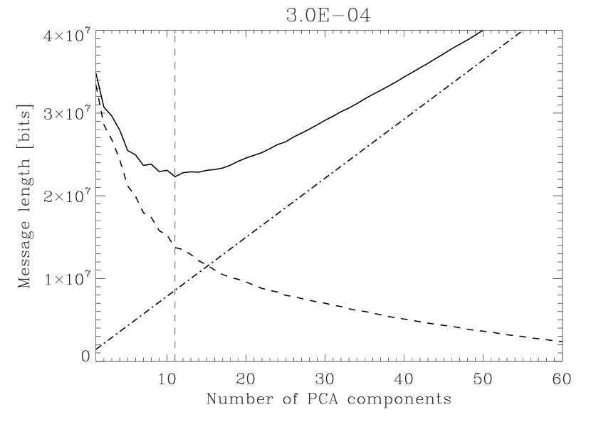
Figure 3.— Application of the MDL criterion to the de-noising of spectropolarimetric signals of quiet Sun observations. The length of the model (dot-dashed line), the data set given the model (dashed line) and the total length (solid line) are plotted versus the number of PCA components included in the data reconstruction for different values of the threshold that sets the precision of the reconstruction (shown in the title of each plot). The vertical dashed line indicates the approximate minimum of the total length curve. Note that the number of PCA components obtained with this MDL criterion increases as the threshold decreases.

Figure 4.— One of the observed Stokes I (left panel) and Stokes V (right panel) profiles is shown in circles. The fits obtained with the two-component model SIR inversion are shown in solid lines. Note that this model is not powerful enough for fitting this strongly asymmetric profiles. Both fits have been obtained using 2 nodes in the temperature. The fit of the Stokes V profiles has been obtained using 4 nodes in the magnetic field strength depth profile.

Figure 5.— Application of the MDL criterion to the selection of the optimum number of nodes in an LTE inversion with the SIR code. The left panel shows the message length when only the number of nodes of the temperature depth profile is changed. The right panel shows the message length when the number of nodes of the magnetic field strength profile is changed.

References

- Akaike (1974) Akaike, H. 1974, IEEE Trans. Autom. Contr., 19, 716
- Gao et al. (2000) Gao, Q., Li, M., & Vitányi, P. 2000, Artificial Intelligence, 121, 1
- Mallows (1973) Mallows, C. L. 1973, Technometrics, 15, 661
- Martínez González et al. (2006) Martínez González, M. J., Collados, M., Ruiz Cobo, B., & Beck, C. 2006, in preparation
- Rees et al. (2000) Rees, D. E., López Ariste, A., Thatcher, J., & Semel, M. 2000, A&A, 355, 759
- Rissanen (1978) Rissanen, J. 1978, Automatica, 14, 465
- Rissanen (1983) —. 1983, The Annals of Statistics, 11, 416
- Rissanen (1986) —. 1986, The Annals of Statistics, 14, 1080
- Rissanen (1989) —. 1989, Stochastic Complexity in Statistical Inquiry (Singapore: World Scientific)
- Ruiz Cobo & del Toro Iniesta (1992) Ruiz Cobo, B., & del Toro Iniesta, J. C. 1992, ApJ, 398, 375
- Sánchez Almeida et al. (1996) Sánchez Almeida, J., Landi degl’Innocenti, E., Martínez Pillet, V., & Lites, B. W. 1996, ApJ, 466, 537
- Shannon (1948a) Shannon, C. E. 1948a, Bell System Tech. J., 27, 379
- Shannon (1948b) —. 1948b, Bell System Tech. J., 27, 623
- Vitányi & Li (2000) Vitányi, P., & Li, M. 2000, IEEE Trans. Inform. Theory, 46, 446