Letter to Editor
On the dependence of the spectral parameters on the observational conditions in homogeneous time dependent models of the TeV blazars

Abstract

Aims. Most of current models of TeV blazars emission assume a Synchrotron Self-Compton mechanism where relativistic particles emit both synchrotron radiation and Inverse Compton photons. For sake of simplicity, these models usually consider only steady state emission. The spectral features are thus only related to the shape of the particle distribution, and do not depend on the timing of observations.

Methods. In this letter, we study the effect of, firstly, the lag between the beginning of the injection of the fresh particles and the trigger of the observation, and secondly, of a finite injection duration. We illustrate these effects considering an analytical time-dependent model of the synchrotron emission by a monoenergetic distribution of leptons.

Results. We point out that the spectral shape can be in fact very dependent on observational conditions if the particle injection term is time-dependent, particularly taking into account the effect of the time averaging procedure on the final shape of the SED. Consequences on the acceleration process are also discussed.

1 Introduction

TeV blazars belong to the radio-loud active galactic nuclei (AGN) and are characterized by non-thermal continuum spectrum, optical polarization, flat radio spectrum and strong variability in all frequency bands. The broad band of the SED which extends from radio up to the TeV range, consists typically in two bumps. The low energy one — peaking in the $0.1-100\rm\ keV$ domain — is commonly attributed to synchrotron emission of ultra-relativistic leptons. In the Synchrotron-Self-Compton process (SSC) the second component is attributed to the inverse Compton (IC) scattering of synchrotron photon field by the same population of leptons. Emission of TeV photons provides evidence for the presence of particles at roughly the same energy if we suppose that they radiate in the IC Klein-Nishina regime (Blumenthal & Gould 1970). Therefore, it requires an extremely efficient particle acceleration mechanism at work in the close environment of supermassive black hole.

Extended observations of TeV blazars like Mrk 501 ($z_{s}=0.034$, Quinn et al. 1996) show that synchrotron component can be very variable in the UV/X-ray range. The simplest approach is the well-known homogeneous or one-zone modeling. It considers the emission of a relativistic moving blob of plasma filled by a tangled magnetic field, where ultra-relativistic particle are injected and can cool freely (via both synchrotron and inverse Compton scattering process). Generally, in these models, the acceleration mechanism is not consistently taken into account and the resulting energy distribution function (EDF) of injected particles is prescribed. If we supposed that the acceleration zone could be dissociated from the radiative one, then we must distinguish two different kinds of EDF : the injected one and the cooled one. In the usual one-zone model, the first is directly the result of the acceleration mechanism. The second ensues from the radiative cooling of particles (and possible re-acceleration mechanism). It is mathematically speaking the solution of the standard kinetic equation which the injected EDF is the main source term. The exact shape of the SED could be only understood in the framework of time dependent modeling, depending on the detail of the cooling and injection processes (Kirk et al. 1998; Chiaberge & Ghisellini 1999). The majority of SSC models are steady-state: therefore the instantaneous SED is equal to the observed one. In this case, the authors use broken power-law EDF as the solution of the kinetic equation (characterized by the indices $\alpha_{\ell}$ and $\alpha_{u}$). Then the subsequent synchrotron spectra have also a broken power-law shape $\mathcal{F}_{\nu}\propto\nu^{-\beta_{\ell,u}}$ with indices $\beta_{\ell,u}=(\alpha_{\ell,u}-1)/2\leqslant 1/3$ over suitable frequency ranges (Blumenthal & Gould 1970). Spectral index variations can arise from the variation of $\alpha_{\ell,u}$ i.e. by varying the physical conditions of the emission zone (see e.g. Kino & Takahara 2004).

We have recently investigated another solution, still in the framework of homogeneous modeling, but with a time dependent particle injection term (Saugé & Henri 2004, , hereafter paper I). The kinetic equation is solved numerically taking into account (i) the possible in-situ pair reprocessing and (ii) both synchrotron and IC cooling term. The source term of the equation is chosen as a quasi-monenergetic distribution of particles (or “pileup”), injected during a finite time. Physically, the formation of such a distribution results from the combination of a stochastic heating via second order Fermi process and radiative cooling (Henri & Pelletier 1991; Schlickeiser 1985). Then the resulting cooled EDF is also partially a power-law, but with a constant index value $\alpha=2$ over a dynamical range depending on the details of the cooling process. In this case, the instantaneous synchrotron spectrum is a power-law of index $\beta=1/2$ and no spectral index variation could be expected at this stage. However, such a variation can be obtained by averaging out the instantaneous SED over the time and considering that the observation starting time does not necessarily coincide with the beginning of injection phase.

In this letter we study in more detail this effect. First of all, we derive a basic model in Sect. 2 in the idealized case of monoenergetic injected EDF subject only to synchrotron cooling. Then we derive the global shape of the time average synchrotron part of the SED as a function of the observational parameters. Finally, we illustrate our approach on BeppoSAX archival data sets of the object Mrk 501 in Sect. 3, before concluding.

2 The model

In the following, all times are expressed in the plasma (blob) rest frame. We neglect the photon flight time across the source by considering evolution only less than $R/c$ where $R$ is the transverse size of the source (see Paper I). This issue was previously studied in detail by Chiaberge & Ghisellini (1999) in the case of the instantaneous emission.

2.1 Energy Distribution Function of Particles

For analytical purpose, we consider the simple case of the injection of a pure monoenergetic EDF of particle of energy $\gamma_{\max,0}$ during a finite time $t_{\rm inj}$

$$\mathcal{Q}_{\rm inj}(\gamma;t)=\mathcal{Q}_{0}\,\delta(\gamma-\gamma_{\max,0})\,\Pi(t;0,t_{\rm inj}),$$ (1)

and we consider that the main channel of particle cooling is the synchrotron process. We also neglect the in-situ pair creation process which can strongly affect the resulting cooled EDF in case of large $\gamma\gamma$-opacity (see Paper I). We introduced the gate function $\Pi(x;x_{\rm min},x_{\rm max})=\Theta(x-x_{\rm min})\Theta(x_{\rm max}-x)$ where $\Theta$ is the usual Heaviside unit step function. We define the cooling time of a particle with a Lorentz factor $\gamma$ by the usual relation $t_{\rm cool}(\gamma)={1}/{k_{\rm syn}\gamma}$, where $k_{\rm syn}={\sigma_{\rm Th}}/{6\pi m_{e}c}B^{2}$. It also represents the time spent by an initial infinite energy particle to cool down to $\gamma$. In the following, another characteristic time value related to the previous one will be $t_{\rm crit}=t_{\rm cool}(\gamma_{\rm max,0})$. Under these assumptions the solution of the standard kinetic equation is analytic : $n(\gamma;t)=n_{0}\gamma^{-2}\Pi(\gamma;\gamma_{\min}(t),\gamma_{\max}(t))$ where the power-law index $2$ is typical of the synchrotron radiative cooling. Values of time-dependent bounds write

$$\gamma_{\min}(t)=\frac{\gamma_{\max,0}}{1+t/t_{{\rm crit}}}\ ;\ \gamma_{\max}(t)=\frac{\gamma_{\max,0}}{1+\max(0,t-t_{{\rm inj}})/t_{{\rm crit}}}.$$ (2)

We also define the dynamical range of distribution as ie the ratio $r_{{\rm dyn}}(t)=\gamma_{\max}(t)/\gamma_{\min}(t)$.

2.2 Instantaneous synchrotron spectrum

As said before, in the case where the previous dynamical range is sufficiently wide, the synchrotron spectrum is itself a power-law of index $1/2$ in $\nu\mathcal{F}_{\nu}$. We recall that a particle of energy $\gamma$ emits preferentially synchrotron radiation roughly at the maximum frequency $\nu_{{\rm s}}(\gamma)=0.29\times{3\gamma^{3}\omega_{s}(\gamma)}/{4\pi}$ where the relativistic synchrotron gyro-frequency writes $\omega_{s}(\gamma)={qB}/{\gamma m_{e}c}$ (Blumenthal & Gould 1970). Then we consider a $\delta$-approximation of the synchrotron kernel function in the optically thin emission limit, centred around $\nu_{{\rm s}}$. In this case, the synthetic synchrotron component SED can be approximated by $\nu\mathcal{F}_{\nu}(t)=S_{0}\nu^{1/2}\Pi(\nu;\nu_{{\rm smin}}(t),\nu_{{\rm smax}}(t))$ over the frequency range given by

$$\left\{\begin{array}[]{rcl}\displaystyle\nu_{{\rm smax}}(t)&=&\displaystyle\frac{\nu_{{\rm smax},0}}{\left[1+\max(0,t-t_{{\rm inj}})/t_{{\rm crit}}\right]^{2}},\\ \displaystyle\nu_{{\rm smin}}(t)&=&\displaystyle\frac{\nu_{{\rm smax},0}}{(1+t/t_{{\rm crit}})^{2}},\end{array}\right.$$ (3)

where $\nu_{{\rm smax},0}=\nu_{{\rm smax}}(t=0)=\nu_{{\rm s}}(\gamma_{\max,0})$.

2.3 Time averaged synchrotron spectrum

As previously said, the observed spectrum results from the time average of instantaneous spectra from $t_{\rm obs}$ to $t_{\rm obs}+\Delta t_{\rm obs}$. The time origin $t=0$ is related to the beginning of the injection of fresh particles. One writes,

$$\langle\nu\mathcal{F}_{\nu}\rangle_{t} = \frac{S_{0}\nu^{1/2}}{\Delta t_{{\rm obs}}}\int_{t_{{\rm obs}}}^{t_{{\rm obs}}+\Delta t_{{\rm obs}}}{\rm d}t\ \Pi(\nu;\nu_{{\rm smin}}(t),\nu_{{\rm smax}}(t)),$$ (4)

$$= \frac{S_{0}\nu^{1/2}}{\Delta t_{{\rm obs}}}\,(\mathcal{I}_{1}+\mathcal{I}_{2}),$$ (5)

where the quantities $\mathcal{I}_{1}$ and $\mathcal{I}_{2}$ arise from the splitting of the previous integral over $[t_{\rm obs},t_{\rm inj}]$ and $[t_{\rm inj},t_{\rm obs}+\Delta t_{\rm obs}]$. After straightforward algebra, these values depend on the position of $t_{{\rm obs}}$ compared to $t_{{\rm inj}}$, and we distinguish two cases,

$$\bullet\ \mbox{case A} : t_{{\rm obs}}\leqslant t_{{\rm inj}}$$

$$\mathcal{I}_{1} = \max[0,t_{{\rm inj}}-\max(t_{{\rm obs}},t_{{\rm crit}}(\nu))],$$

$$\mathcal{I}_{2} = \min[t_{{\rm obs}}+\Delta t_{{\rm obs}},t_{{\rm inj}}+t_{{\rm crit}}(\nu)]-\max[t_{{\rm inj}},t_{{\rm crit}}(\nu)],$$

$$\bullet\ \mbox{case B} : t_{{\rm obs}}\geqslant t_{{\rm inj}}$$

$$\mathcal{I}_{1} = 0,$$

$$\mathcal{I}_{2} = \min[t_{{\rm obs}}+\Delta t_{{\rm obs}},t_{{\rm inj}}+t_{{\rm crit}}(\nu)]-\max[t_{{\rm obs}},t_{{\rm crit}}(\nu)].$$

where we define $t_{{\rm crit}}(\nu)=t_{{\rm crit}}\times[({\nu_{{\rm smax},0}}/{\nu})^{1/2}-1]$ representing the time needed by the lower bound of the synchrotron spectrum to reach the frequency $\nu$.

3 Results and Discussion

3.1 Effects of parameters

Using the previous relations, we show the influence of the $t_{\rm obs}$ parameter on the time averaged spectra on Fig. 1. On theses figures, the time is normalized in unit of $t_{\rm inj}$ and frequency in unit of $\nu_{\rm smax,0}$. If $t_{\rm obs}+\Delta t_{\rm obs}>t_{\rm inj}$, the resulting SED consists of two parts (see left panel). The lower one exhibits a power-law tail of constant index $1/2$ and results from the emission of most energetic particle injected since the start of the observation (and not from the beginning of the injection) and which have not yet had the time to cool. Conversely, up to $\nu_{{\rm break}}$ the spectrum softens. In this case we obtain from (3) $\nu_{{\rm break}}=\nu_{\rm smax}(t_{\rm obs})$ or explicitly

$$\nu_{{\rm break}}(t_{\rm obs})=\frac{\nu_{{\rm smax},0}}{(1+t_{{\rm obs}}/t_{{\rm crit}})^{2}}.$$ (6)

In the case $t_{\rm obs}\leqslant t_{\rm inj}\leqslant t_{\rm obs}+\Delta t_{\rm obs}$, the high energy part could be also described by a power-law with local index $\alpha$, which implicitly depends on $t_{\rm obs}$. Combining previous calculations, we obtain

$$\alpha = \frac{\log\left[\langle\nu\mathcal{F}_{\nu}\rangle(\nu_{\rm smax,0})/\langle\nu\mathcal{F}_{\nu}\rangle(\nu_{\rm break})\right]}{\log\left[\nu_{\rm smax,0}/\nu_{\rm break}\right]}$$ (7)

$$= \frac{\log\left[\left(1-t_{\rm obs}/t_{\rm inj}\right)\left(1+t_{\rm obs}/t_{\rm crit}\right)\right]}{2\log\left(1+t_{\rm obs}/t_{\rm crit}\right)}\leqslant\frac{1}{2}\left(1-\frac{t_{\rm crit}}{t_{\rm inj}}\right)$$ (8)

where the upper bound is obtained for $t_{\rm obs}=0$. Note that the spectrum is expected to be flat ($\alpha=0$) when $t_{\rm obs}=t_{\rm inj}-t_{\rm crit}$.

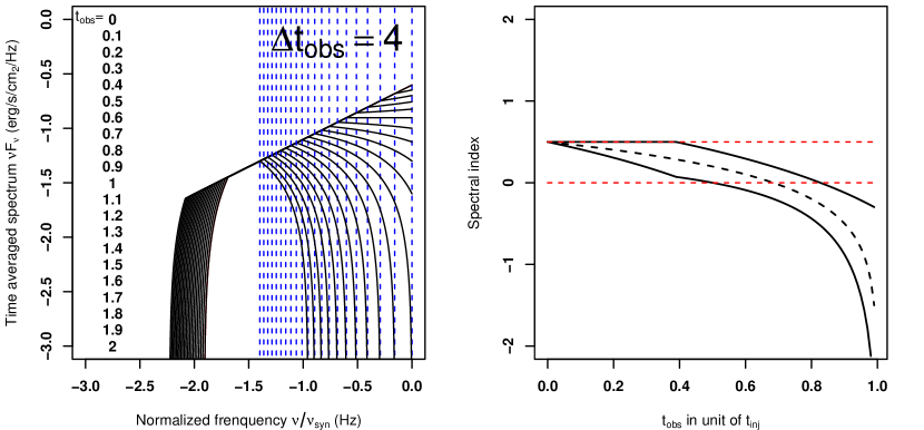
Figure 1: Influence of the value of $t_{\rm obs}$ parameter on the time averaged SED (left panel) with $\Delta t_{\rm obs}=4t_{\rm inj}$ and $t_{\rm crit}=0.5t_{\rm inj}$. Vertical dashed lines represent location of the frequency break $\nu_{\rm break}$ calculated for each previous curve (see eq. [6]). Resulting local spectral indices in normalized frequency range $[-0.5,0]$ (upper solid curve), $[-1,-0.5]$ (lower solid curve) and $[-1,0]$ (dashed curve) are given on the right panel.

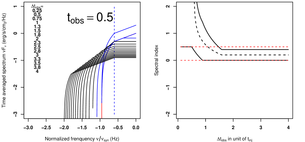
Figure 2: Same as Fig. 1 for the influence of the $\Delta t_{\rm obs}$ parameter with $t_{\rm obs}=t_{\rm crit}=0.5t_{\rm inj}$. Considering these parameter values, we easily verify that spectral index above $\nu_{\rm break}=0.25\,\nu_{\rm smax,0}$ is going to be flat since $\Delta t_{\rm obs}\geqslant t_{\rm inj}-t_{\rm obs}=0.5$.

This mechanism gives a plausible explanation of the broken power-law or curved shape of TeV blazars reported by many authors (see e.g. Fossati et al. 2000a, b). Following our study, we deduce that the low energy synchrotron index should be always be equal to $1/2$ in $\nu\mathcal{F}_{\nu}$ representation. Up to $\nu_{\rm break}$, the index value strongly depends both on the observational characteristics and on the details of the cooling process. Moreover, for $t_{\rm obs}\gg t_{\rm inj}-t_{\rm crit}$, this part of the SED strongly steepens and akin to a pure power-law. It is interesting to note that the maximum curve naturally moves from $\nu_{\rm smax,0}$ to $\nu_{\rm break}$ as the time increases and strongly depends on the value of observational parameters. Right panel shows the time evolution of spectral index calculated in three different logarithmic frequency bands, namely $[-0.5,0]$, $[-1,-0.5]$ and $[-1,0]$.

Similarly, Fig. 2 shows the main effects of the increase of the $\Delta t_{\rm obs}$ parameter. In the case of $t_{\rm obs}\leqslant t_{\rm inj}\leqslant t_{\rm obs}+\Delta t_{\rm obs}$, the spectral shape does not evolve. As expected, only the global flux level changes (decreasing linearly with $\Delta t_{\rm obs}$) just as the low-frequency cut-off (decreasing as maximum system time $t_{\rm obs}+\Delta t_{\rm obs}$ increases).

3.2 Application to Markarian 501

Mrk 501 is a privileged TeV blazar target. It has been studied extensively during many multi-wavelength campaigns and have been observed in various spectral states. We now test our simple approach on state extracted from the BeppoSAX mission public archive . In the following we consider three different data sets, two from the 1997 April flaring period (Pian et al. 1998) and one from the 1999 June period (Tavecchio et al. 2001). Corresponding SED are given in Fig. 3. The two first SED have been studied in Paper I with the more complete homogeneous SSC model and using high-energy data in order to constrain all physical quantities.

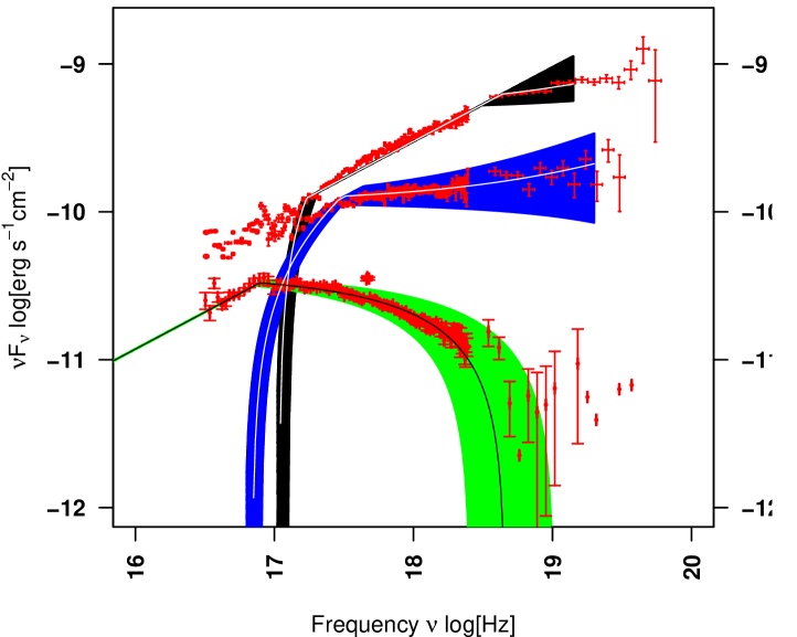
Figure 3: Fits of Markarian 501 UV/X-ray synchrotron spectrum for three different periods.

Table 1: Parameters used in our simulations. All times are expressed in unit of $t_{\rm inj}$

data sample	$t_{\rm crit}$		$t_{\rm obs}$		$\Delta t_{\rm obs}$
		min	max	est
1997 April 7	0.1095	0.68	0.92	0.8	0.946
1997 April 16	0.438	0	0.5	0.35	4.2
1999 June	0.0512	1.05	1.15	1.1	4.5

All parameter values needed for the synchrotron part of the SED fits and suitable estimations are given in Table 1. Again, the times are expressed in unit of $t_{\rm inj}$. For each period, we represent a continuous set of curves as the function of $t_{\rm obs}$ ; also represented, our best estimation of $t_{\rm obs}$.

3.2.1 1997 April period

For the 1997 April 16 (medium state) and April 7 (high state) observations, we find of course values quite similar to Paper I. Fits are very good except for the extreme high energy part of the spectra. The exact form of this cut-off depends both on the exact profile synchrotron kernel and on the exact shape of the particle cooled EDF which are rather approximate in this work. For both periods, the beginning of the observation takes place before the end of the injection phase and therefore the synchrotron spectra displays a positive $\alpha$ value, as defined in equation (7).

First analysis done by Pian et al. (1998) using an one-zone model with a power-law injection function show that the April 16 spectrum is correctly reproduced for an injected EDF with an index $s=1$ over a dynamical range less than 10. In the usual context of shock acceleration process, the value of the index $s$ case, the index $s$ directly depends on the physical conditions at the shock (Blandford & Ostriker 1978; Protheroe & Stanev 1999),

$$s=1+\frac{t_{\rm acc}}{t_{\rm esc}}=\frac{R+2}{R-1}\ >1.$$ (9)

In the last expression, $t_{\rm acc}$ and $t_{\rm esc}$ are respectively the acceleration and the escape characteristic time, and $R$ the shock compression ratio. Then the value $s=1$ is highly unlikely, because it requires $t_{\rm esc}\to\infty$, which is not consistent : particles can not escape from the accelerator. Moreover, the narrowness of the dynamical range in this latter case clearly pleads for a monoenergetic injection function and consequently for a stochastic acceleration process.

In classical shock acceleration model, the difference between the 1997’s high and medium state is explained by difference in the shock physical condition — e.g. via the compression ratio $R$ — leading to a different index value $s$. In the light of our scenario and as already noted in Paper I, the difference in the shape of the spectra arises essentially from different observational conditions. The medium state corresponds to a previous injection observed in a later stage (with respect to beginning of the injection phase). This is corroborated by the flatness of the high energy part of the X-ray spectrum.

3.2.2 1999 June period

During 1999 June period the synchrotron spectrum experienced a very steep state. In the context of the power-law injected EDF, this state is explained with a large value of the index $\alpha_{u}$ of the upper part of the EDF, roughly equals to $4.3$ (Tavecchio et al. 2001).

In the shock acceleration scenario the value of $\alpha_{u}$ is related to $s$ via the relation $\alpha_{u}=s+1$ (Kino & Takahara 2004). Then in our precise case,it corresponds to an acceleration time quite larger than the escape one ($t_{\rm acc}=3.3\,t_{\rm esc}$ or, in term of compression ratio $R\approx 1.9$). In our approach, this spectral shape is obtained considering an observation time $t_{\rm obs}$ larger than $t_{\rm inj}-t_{\rm crit}\approx t_{\rm inj}$.

4 Conclusion

We have exposed a simple time dependent mechanism in order to explain the spectral shape of the synchrotron spectrum of blazar considering the injection of a pure monoenergetic distribution of ultra-relativistic particles over a finite time range. This latter EDF arises from stochastic acceleration mechanism (Second order Fermi process). Spectral index and SED shape variations can be explained by the value of the starting observation time with respect to the beginning of the injection of fresh particles and from the variation of the acceleration condition even if the instantaneous synchrotron spectrum is universal with a constant spectral index equals to $1/2$. Because blazars are extremely variable sources, there are often observed in “Target-of-Opportunity” mode, where satellites observations are triggered by some other instruments after some delay leading naturally to $t_{\rm obs}\neq 0$. This mechanism leads to complex time dependent behaviors of the spectral shape ; we show that we can reproduce various spectral shapes from the single to broken power-law shape, with strong or soft cut-off. This model differs from the usual one in the context of the shock acceleration model, where the spectral variability arises from the physical conditions at the shock.