Inflation and WMAP three year data: Features have a Future!

Abstract

The new three year WMAP data seem to confirm the presence of non-standard large scale features in the cosmic microwave anisotropy power spectrum. While these features may hint at uncorrected experimental systematics, it is also possible to generate, in a cosmological way, oscillations on large angular scales by introducing a sharp step in the inflaton potential. Using current cosmological data, we derive constraints on the position, magnitude and gradient of a possible step. We show that a step in the inflaton potential, while strongly constrained by current data, is still allowed and may provide an interesting explanation to the currently measured deviations from the standard featureless spectrum. Moreover, we show that inflationary oscillations in the primordial power spectrum can significantly bias parameter estimates from standard ruler methods involving measurements of baryon oscillations.

I Introduction

The recent three year results from the Wilkinson Microwave Anisotropy Probe (WMAP) satellite wmap3cosm ; wmap3pol ; wmap3temp ; wmap3beam have further confirmed with an extraordinary precision the inflationary paradigm of structure formation in which primordial fluctuations are created from quantum fluctuations during an early period of superluminal expansion of the universe Starobinsky:1979ty ; muk81 ; bardeen83 .

Indeed, soon after the WMAP data release, a number of authors investigated the possibility to discriminate between several single-field inflationary models using this new, high quality, dataset alabidi ; PeirisEasther ; Lewis:2006ma ; Seljak:2006bg ; Magueijo:2006we ; Liddle06 ; kinney06 ; Martin:2006rs . One of the main conclusions of these works is that some inflationary models, such as quartic chaotic models of the form $V(\phi)\sim\lambda\phi^{4}$, may be considered ruled out by the current data, while others, such as chaotic inflation with a quadratic potential $V(\phi)\sim m^{2}\phi^{2}$, are consistent with all data sets.

One important assumption in these analyses (apart for Martin:2006rs ) is that the inflaton’s potential is featureless, i.e., there is no preferred scale during inflation and the primordial power spectrum of density perturbations in Fourier $k$-space can be well approximated by a power law $k^{n}$, where the spectral index $n$ is almost scale independent. The main prediction of these models is that the anisotropy angular power spectrum should be “smooth” and not show features in addition to those provided by the baryon-photon plasma oscillations at decoupling within the framework of the standard $\Lambda$CDM model of structure formation.

The current WMAP data is in very good agreement with this hypothesis: several non-standard features in the anisotropy angular power spectrum detected in the first year data have now disappeared thanks to the longer integration time of the observations and better control of systematics (see wmap3cosm ).

However, features in the large scale anisotropy spectrum are still present in the new release. Moreover, some of the cosmological parameters derived from the new WMAP data, like, for instance, the low value of the variance of fluctuations $\sigma_{8}$, appear in tension with those derived by complementary data sets. It is therefore timely to investigate a larger set of inflationary models and to consider a cosmological origin of these unexpected features.

A departure from power law behavior of the primordial power spectrum could be caused by a change of the initial conditions, due to trans-planckian physics Martin:2003kp ; Easther:2002xe or unusual initial field dynamics Burgess:2002ub ; Contaldi:2003zv or by some brief violation of the slow roll conditions during inflation Kofman:1989ed ; Starobinsky:1992ts . We will investigate a model of the second type where features in the temperature and density power spectra arise due to a step-like change in the potential parameters, as proposed by ace . A sharp step in the inflaton mass, caused, e.g., by a symmetry breaking phase transition, generates indeed $k$-dependent oscillations in the spectrum of primordial density perturbations.

The goal of our paper is to make use of the recent three year WMAP data (WMAP3) and other datasets to constrain the possibility of a step feature in the inflaton potential. For this purpose we adopt the phenomenological model proposed by Adams et al. ace , where a step feature is added to the chaotic inflationary potential in the following way:

$$V(\phi)={1\over 2}m^{2}\phi^{2}\,\left(1+c\tanh\left(\frac{\phi-b}{d}\right)\right),$$ (1)

where $m$ is an overall normalization factor, $c$ determines the height of the step, $d$ its gradient and $b$ is the field value on which the step is centered. Previous phenomenological studies of the same Peiris:2003ff or other oscillatory features Martin:2004yi ; Kawasaki:2004pi have been limited to the first year WMAP data, and in general a full analysis varying also all cosmological parameters is still missing and is the major result of this work.

The paper is organized as follows: In Sec. II we briefly review step-inflation models. In Sec. III we describe our analysis method. In Sec. IV we present our results and, finally, in Sec. V we derive our conclusions.

II Inflation models with a step in the potential.

Inflationary models with a step can naturally arise in theories with many interacting scalar fields, e.g., in supergravity models. In general, these models contain several flat directions in field space and thus offer the possibility to have multiple inflationary phases separated by phase transitions ars97 , or even inflation with a curved trajectory in field space mukh98 ; star01 ; groot01 . In the last case the presence of additional active scalar degrees of freedom generates not only the adiabatic mode of curvature perturbations, but also the isocurvature one. Since the data do not seem to require an isocurvature component isobound , we will restrict ourselves to the case where the phase transition does not appreciably change the rolling direction corresponding to the inflaton field and the energy density is always dominated by a single field. Also, we will investigate the simplest scenario and assume that the sole effect of the phase transition is to change the parameters of the Lagrangian for the inflaton field, in particular its mass.

Consider a hybrid inflationary potential of the type

$$V=V_{0}+{1\over 2}m_{0}^{2}\phi^{2}+{\lambda^{2}\over 4}\left(\psi^{2}-M^{2}\right)^{2}+\lambda^{2}\phi^{2}\psi^{2}\;,$$ (2)

where $\phi$ is the inflaton field, while $\psi$ is a hybrid field that takes a vacuum expectation value during inflation when the inflaton reaches the critical value $\phi_{c}^{2}={M^{2}\over 2}$. In the usual case of hybrid inflation, this transition is so strong that it stops the inflationary phase. But, if the coupling $\lambda$ is sufficiently small, the back-reaction of $\psi$ is too weak and inflation continues. On the other hand, the parameters of the Lagrangian change their value and for example the inflaton effective mass becomes

$$m_{\text{eff}}^{2}(\phi)=m_{0}^{2}+\lambda^{2}\langle\psi^{2}\rangle(\phi)\;.$$ (3)

In this scenario, even if the classical inflaton is nearly unperturbed, the inflaton perturbations are affected and the primordial power spectrum is modified.

It is well known that a step in the mass generates oscillations in the primordial spectrum and this can be described analytically in the WKB approximation hs04 . The behavior of the inflaton mass is determined by the dynamics of the phase transition and the growth of the hybrid field fluctuations, which become tachyonic after the critical point. This growth depends on the classical inflaton field motion, but is in general so fast that $\psi$ reaches the minimum in a very small number of $e$-foldings fggklt01 ; abc01-hyb ; cpr02 ; ggg02 . The inflaton mass is therefore reasonably well approximated by a hyperbolic tangent, and so we take

$$m_{\text{eff}}^{2}(\phi)\simeq m^{2}\left(1+c\tanh\left(\frac{\phi-b}{d}\right)\right).$$ (4)

Here, we see that the parameter $m$ is an average inflaton mass and $b$ is of the order of the critical value $\phi_{c}$. The other two parameters determine the duration of the transition and the strength of the effect on the inflaton’s mass. Note that we work in Planck units, so all dimensional quantities like $b$ and $d$ should be multiplied by $M_{\text{P}}$ in order to obtain their value in physical units. In this article we restrict ourselves to the case of chaotic inflation, where the mass term determines both the classical dynamics of the inflaton and the behavior of the perturbations. A more general discussion will be left for a longer publication chmss2 . We therefore assume that $V_{0}$ and also its change due to the phase transition are completely negligible. We also discuss here only positive $c$ values; negative $c$ is also allowed, but is restricted to be very small to avoid the presence of another minimum in the potential away from $\phi=0$.

Since we cannot rely on the slow roll approximation for a generic choice of parameters, we integrate the equations for the background and for the modes numerically as discussed in detail in ace . The equations for the inflaton field and the Hubble parameter in Planck units are simply

$$\ddot{\phi}+3H\dot{\phi}+V^{\prime}(\phi)=0$$ (5)

$$3H^{2}={\dot{\phi}^{2}\over 2}+V(\phi).$$ (6)

We assume slow roll as the initial condition for $\phi\gg\phi_{c}$ and solve the evolution numerically until the end of inflation in order to determine the number of $e$-foldings between $b$ and the end of inflation.

The equation for the Fourier components of $u=-z{\cal R}$, the curvature perturbation Stewart:1993bc , takes the usual form

$$u_{k}^{\prime\prime}+\left(k^{2}-{z^{\prime\prime}\over z}\right)u_{k}=0$$ (7)

where $z=a\dot{\phi}/H$ is given by the background dynamics and the primes and dots denote derivatives with respect to conformal time and physical time, respectively. Using the equations of motion for the classical field, we have in general

$${z^{\prime\prime}\over z}=2a^{2}H^{2}\left(1+{7\dot{\phi}^{2}\over 4H^{2}}+{\dot{\phi}^{4}\over 4H^{4}}+{V^{\prime}\dot{\phi}\over H^{3}}-{V^{\prime\prime}\over 2H^{2}}\right),$$ (8)

where $V^{\prime}$ and $V^{\prime\prime}$ are the derivatives of the potential with respect to the inflaton field. In the step model, this quantity can deviate substantially from the slow-roll expectation $z^{\prime\prime}/z\simeq 2a^{2}H^{2}$ at the time of the transition. We solve equations (5) to (7) numerically using a Bulirsch-Stoer algorithm for free field initial conditions at an initial time when $k^{2}\gg z^{\prime\prime}/z$ is satisfied.

Once we know the solution for the mode $k$, we can determine the primordial power spectrum

$$\mathcal{P_{R}}(k)={k^{3}\over 2\pi}\left|\frac{u_{k}}{z}\right|^{2},$$ (9)

evaluated when the mode is well outside the horizon. Our results are stable with respect to changes in the exact time when we set the initial conditions and when we compute the spectrum.

Figure 1: Effects of a step in the potential on the power spectrum of curvature perturbations. Here we show the primordial spectrum for the two best fit points, corresponding to $b=14.81$, $c=0.0018$, $d=0.022$ (dashed line) and $b=14.34$, $c=0.00039$, $d=0.006$ (solid line).

The resulting spectra as a function of $k$ for different parameters are shown in Figure 1. Essentially, the spectrum shows a power-law behavior with a superimposed oscillation.

How will the four parameters of our model affect the shape of the spectrum? The overall normalization of $\mathcal{P_{R}}$ is proportional to $m^{2}$, $b$ determines the wavelength at which the feature appears and the maximum amplitude of the oscillations is roughly proportional to $c$. Generally, the dominant contribution to $z^{\prime\prime}/z$ comes from the $V^{\prime\prime}$ term and is proportional to $c/d^{2}$, so the range of $k$ affected by the feature depends on the square root of $c/d^{2}$. Note that away from the step, the slow roll conditions are satisfied and the spectrum recovers the usual power law form with spectral index given by $n_{s}=1-2/N\simeq 0.96$ for a number of $e$-foldings $N$ equal to 50, which is what we assume for our analysis. The value of the spectral index is the same before and after the step since it does not depend on $m^{2}$ in $m^{2}\phi^{2}$ models. Also, for values of the parameters where the slow-roll conditions are always satisfied (i.e., small values of $c/d^{2}$), the spectrum does not show a full oscillation, but a dip at the scales corresponding to the transition. So even in this case it is not so well approximated by the usual power-law with a constant spectral index.

III CMB Analysis

We compare the theoretical model described in the previous sections with a set of current cosmological data by making use of a modified version of the publicly available Markov Chain Monte Carlo (MCMC) package cosmomc Lewis:2002ah .

We sample an eight-dimensional set of parameters. Four of them determine the primordial power spectrum, namely the $b,c$ and $d$ parameters of the step-inflation model as described in the previous section and the overall normalization of the primordial power spectrum $A_{S}$ (equivalent to $m^{2}$ as discussed earlier). The remaining four cosmological parameters are the physical baryon and CDM densities, $\omega_{b}=\Omega_{b}h^{2}$ and $\omega_{c}=\Omega_{c}h^{2}$, the ratio of the sound horizon to the angular diameter distance at decoupling, $\theta_{s}$ and finally, the optical depth to reionization, $\tau$. Furthermore, we consider purely adiabatic initial conditions, impose flatness and neglect neutrino masses.

We include the three year data wmap3cosm (temperature and polarization) using the likelihood routine for supplied by the WMAP team and available at the LAMBDA web site. We marginalize over the amplitude of the Sunyaev-Zel’dovich signal. The MCMC convergence diagnostics are done on four chains using the Gelman and Rubin “variance of chain means”$/$“mean of chain variances” $R$ statistics for each parameter, demanding that $R-1<0.1$. Our $2D$ constraints are obtained after marginalization over the remaining “nuisance” parameters, again using the programs included in the cosmomc package.

In addition to CMB data, we also consider the constraints on the real-space power spectrum of galaxies from the Sloan Digital Sky Survey (SDSS) thx .

We restrict the analysis to a range of scales over which the fluctuations are assumed to be in the linear regime ($k<0.2\;h/{\text{Mpc}}$). When combining the matter power spectrum with CMB data, we marginalize over an additional nuisance parameter $b^{\prime}$, the dark versus luminous matter bias. Furthermore, we make use of the HST key project measurement of the Hubble parameter $H_{0}=100h\text{ km s}^{-1}\text{Mpc}^{-1}$ hst by multiplying the likelihood by a Gaussian centered around $h=0.72$ with a standard deviation $\sigma=0.08$. Finally, we impose a top-hat prior on the age of the universe, $10<t_{0}<20$ Gyrs, and a Gaussian prior on $\Omega_{b}h^{2}$ centered around $0.022$ with a standard deviation of $0.002$ from BBN constraints, cf. Ref. Lewis:2002ah .

We demand that the feature appear at a wavelength to which our data is sensitive, so our analysis will be limited to the interval $13.5<b<16$. Apart from that we also impose logarithmic priors on the other step parameters: $\log c\in[-6,-1]$, $\log d\in[-2.5,-0.5]$ and $\log c/d^{2}\in[-5,3]$ and flat priors on the cosmological parameters.

As it turns out, the likelihood distribution $\mathcal{L}$ has a rather odd shape and some of the interesting features are at low likelihoods. In order to improve mixing and get a better coverage of the low likelihood regions, we sample $\mathcal{L}^{1/3}$ instead of $\mathcal{L}$ (i.e., we use “heated” chains at $T=3$).

As a measure of the performance of the step model, we compare its best fit $\chi^{2}$ with the best fit $\chi^{2}$ of a reference model, which we take to be the “vanilla” 6 parameter ($\Omega_{b}h^{2}$, $\Omega_{c}h^{2}$, $\theta_{s}$, $\tau$, $A_{S}$ and $n_{s}$) power law $\Lambda$CDM model.

IV Results

Figure 2: Marginalised likelihood (solid line) and projection of the likelihood distribution (dotted line) for the $b$ parameter in the case of WMAP only. Two peaks for $b$ at $b=14.3$ and $b=14.8$ are clearly visible. The one at $b=14.8$ provides a good fit to the low $\ell$ WMAP glitches. It is evident that the likelihood function is far from gaussian in this direction. The difference between the two curves is caused by a volume effect when integrating over the other parameter directions.

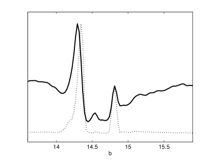
Let us first consider the WMAP dataset alone. In Figure 2 we plot the mean likelihood for the $b$ parameter which determines the position (scale) of the step in the potential. If some value of $b$ is preferred by the data, then it would hint at the presence of a feature. As we can see, the mean likelihood distribution clearly indicates two maxima for the $b$ parameter at $b=14.3$ and $b=14.8$, respectively. The feature at $b=14.8$ is able to produce a good fit to the WMAP low-$\ell$ glitches (yielding an improvement of $\Delta\chi^{2}\simeq 5$ over the vanilla model) and agrees with the results of Ref. Peiris:2003ff for fixed cosmological parameters and WMAP first year data. Interestingly, the authors of Shafieloo:2003gf find an oscillating feature at roughly the same scale by reconstructing the primordial power spectrum from the first year data. The minimum at $b=14.3$ provides oscillations on smaller scales ($\Delta\chi^{2}\simeq 7$), beyond the second peak in the anisotropy power spectrum, see Figure 3.

Figure 3: This plot shows the temperature anisotropy angular power spectrum of the best fit step model (WMAP only, solid line) and, for reference, the best fit 6 parameter power law $\Lambda$CDM model (dashed line). The dotted line shows the effect of a feature near $b=14.8$ for WMAP data only, i.e., the “local” best fit at the lower peak in Figure 2.

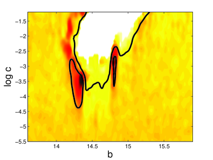
It is interesting to project the likelihood function onto the $(b,\,\log c)$ plane (Figure 4, upper panel). First of all, we see that for a range of values ($14.3<b<15.5$) a region of step models with $\log c$ $<-3$ is ruled out at $99\%$ confidence level. This disfavored region corresponds to the region in $k$ space that is better sampled by the WMAP data, and where, therefore, the data provide the strongest constraints. Secondly, the two aforementioned maxima in $b$-space can again be seen in the $2D$ projection. These maxima are close to the two boundaries (large and small scales) of the region sampled by WMAP and centered around amplitude $\log c\sim-3$. We find that the WMAP polarization and cross temperature-polarization data are rather insensitive to the presence of features.

Figure 4: Mean likelihood and marginalized likelihood contours in the ($b,\,c$) and $(b,\,c/d^{2})$ planes at $8\%$ and $99\%$ c.l. for WMAP data only. The peaks comprise less than ten per cent of the total volume of the likelihood function.

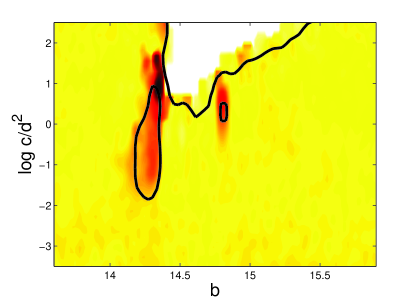
The $d$ parameter is not well constrained by the data due to a degeneracy with $c$. Instead, we consider the constraints in the ($b,\,\log c/d^{2}$) parameter space (Figure 4, bottom panel). This parameter is as well constrained as $c$ and, again, the presence of two maxima for $b$ is evident. Also, the maxima are at values of $c/d^{2}$ of order $1$, where the slow-roll conditions are strongly violated; values of $c/d^{2}\ll 0.1$ correspond, on the other hand, to the usual slow-roll $m^{2}\phi^{2}$ inflation and cannot be excluded by the data.

Note that in the ($b,c,d$)-subspace of parameter space the likelihood function is very oddly shaped and can by no means be approximated by a multivariate Gaussian. As a consequence, the likelihood at the boundaries of this subspace is generally not negligible (see, e.g., Figure 2). In fact, the likelihood function will have a large plateau of constant likelihood in regions where the step model cannot be distinguished from the $m^{2}\phi^{2}$ chaotic inflation model, either because the step is too small or too smooth (small $c$, large $d$) or because the feature appears at wavelengths the data is not sensitive to ($b$ too small or too large). Apart from the two peaks, we also find a valley that can be excluded at a high confidence level. However, since the plateau may contain a significant fraction of the total volume of the likelihood distribution, constraints derived from marginalization will be dependent on the priors on $b$, $c$ and $d$.

Figure 5: Likelihood contours in the $(b,\,c)$ and $(b,\,c/d^{2})$ planes at $68\%$ and $99\%$ confidence level for CMB+SDSS.

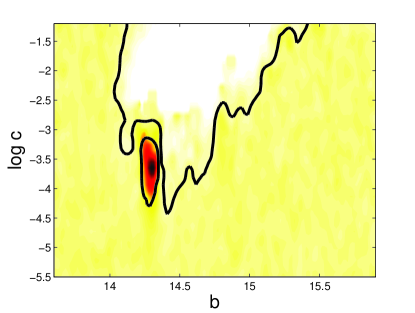
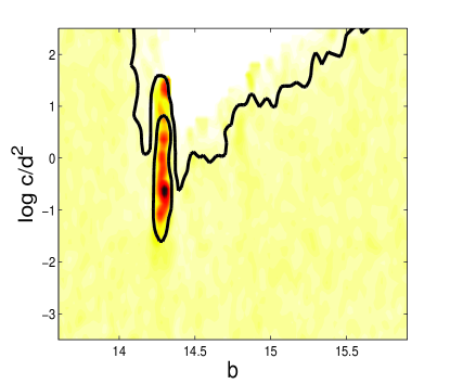
For our choice of priors and WMAP data only, we find that the peak regions contribute about $8\%$ of the total volume, so, from a Bayesian standpoint, the WMAP data alone do not require the presence of a feature.

Figure 3 indicates that the best fit model has a feature at a range of wavelengths where the WMAP data are limited by large systematic errors. It is therefore interesting to enquire whether the inclusion of other data sets which are more sensitive at small scales will corroborate this result. To this end we add small scale CMB data from the ACBAR, BOOMERANG, CBI, MAXIMA and VSA experiments acbar ; boom ; cbi ; maxi ; vsa and the SDSS large scale structure data.

These data sets probe mainly smaller scales and are not sensitive to the large scale feature at $b=14.8$.

We find that including these small scale data improves the constraints on the oscillations quite significantly: $\Delta\chi^{2}\simeq 15$, to which the SDSS data alone contribute about 6. As we can see from Figure 6 (bottom panel), step-induced oscillations in the matter power spectrum seem to provide a much better fit to the SDSS data.

Figure 6: Top: temperature anisotropy angular power spectrum with small scale CMB data.
Bottom: galaxy power spectrum and the SDSS data.
The solid lines depict the best fit step model, the dashed line the best fit reference model.

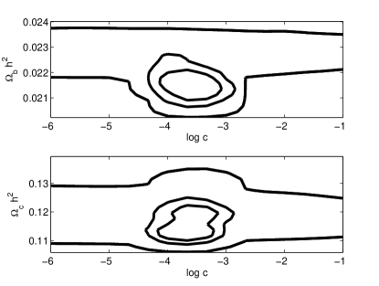
In Figure 5 we plot the likelihood contours in the ($b,\log c$) plane at $68\%$ and $99\%$ c.l. for the CMB+SDSS case. Adding the SDSS data increases the statistical significance of the maximum, the peak near ($b\simeq 14.3$ , $\log c\simeq-3.5$, $\log c/d^{2}\simeq 0$) now contains about $70\%$ of the total volume of the likelihood function, the likelihood at the boundaries of parameter space is suppressed and hence, the results are much less prior dependent. Also, we can rule out a much larger chunk of parameter space for $b<14.5$ due to the increased sensitivity of the data on the corresponding scales.

The variance test convergence stats using last half chains are $0.0007$ for $b$, $0.0038$ for $\log c$ and $0.0036$ for $\log c/d^{2}$, showing a robust convergence of the chains.

We also considered data from the 2dF Galaxy Redshift Survey Cole:2005sx and we found that the CMB+SDSS results are stable under the inclusion of the 2dF dataset.

Of course, oscillatory behavior in the observed data could well have its origin in uncorrected or unidentified systematic effects such as a scale dependent bias. However, as indicated by our results, the presence of multiple step-like features in the inflaton potential (expected from, e.g., supergravity or M-theory models Ashoorioon:2006wc ) is also a viable solution.

It is important to check if the step in the potential suggested by the CMB+SDSS analysis has some impact on the estimation of the remaining cosmological parameters. We find no correlations between $b,c,d$ and the cosmological parameters $A_{S},\theta_{s}$ and $\tau$. This is clearly due to the fixed spectral index the model has away from the feature.

On the other hand some correlation is present between $c$ and the baryon and cold dark matter energy densities $\Omega_{b}h^{2}$ and $\Omega_{c}h^{2}$. Figure 7 shows the confidence level likelihood contours in the $(\Omega_{b}h^{2},c)$ and $(\Omega_{c}h^{2},c)$ parameter space. A deeper step in the potential (larger $c$) has the effect of making the data more compatible with a lower baryon density and a higher cold dark matter density. While the effect is small, it is interesting to note that the baryon density derived from the WMAP data in the framework of the standard model is generally larger than that predicted by standard big bang nucleosynthesis and measurements of the primordial deuterium abundance (see, e.g., fields ).

Figure 7: Correlations between $c$ and the cosmological parameters $\Omega_{b}h^{2}$ and $\Omega_{c}h^{2}$ for CMB+SDSS. Plotted are the $50\%$, $68\%$ and $99\%$ confidence levels. The best fit step model peak prefers a slighly lower value of $\Omega_{b}h^{2}$ than the plateau region where the feature is insignificant. One can also see that near the best fit region, the larger $c$ the smaller the corresponding value of $\Omega_{b}h^{2}$.

V Mimicking Baryonic Oscillations

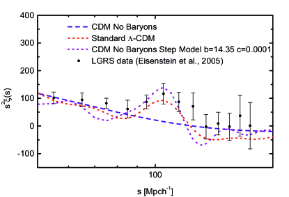
Recently, a detection of oscillations in the correlation function of the Luminous Red Galaxies sample of the SDSS has been reported in eisenstein . If those oscillations are the imprint of primordial acoustic oscillations in the primeval baryon+photon plasma, then they may provide a standard ruler at the redshift of the survey and a very powerful tool for testing the late time evolution of the universe and, ultimately, the appearance of dark energy. Clearly, if oscillations in the primordial spectrum are present they may mimic baryonic oscillations Wang:2002hf at different scales and drastically change the estimation of cosmological parameters.

As a qualitative example, we plot in Figure 8 the correlation functions for a model with no baryons, the standard $\Lambda$CDM model ($\Omega_{b}=0.05$) and a model with no baryons but with a step in the inflationary potential. As we can see, a model with no baryons but with oscillations in the primordial spectra can reproduce the observed data very well. A more detailed and quantitative analysis will be presented in a future paper chmss2 .

Figure 8: Correlation functions for a model with no baryons, the standard $\Lambda$CDM model ($\Omega_{b}=0.05$) and a model with no baryons but with a step in the inflationary potential. The data points are from the LRGS sample of eisenstein .

VI Conclusions

The new three year WMAP data seem to confirm the presence of non-standard large scale features on the cosmic microwave anisotropy power spectrum. While these features may hint at uncorrected experimental systematics, a possible cosmological way to generate large angular scale oscillations is to introduce a sharp step in the inflaton potential. By making use of current cosmological data we derive constraints on the position, magnitude and gradient of a possible step in the inflaton potential. Our conclusion is that such a step, while strongly constrained by current data, is still allowed and may provide an interesting explanation to the current measured deviations from the standard featureless spectrum at low $\ell$.

Surprisingly though, the combination of all CMB data sets with the SDSS data seems to prefer a feature at small scales, which could mimic the effect of baryonic oscillations and reduces the best fit value of $\Omega_{b}$. Note that for this it is sufficient to have a minute change, of order $0.1\%$, in the inflaton mass parameter, but a relatively fast one.

It is an open question if such a sharp step can be realized in realistic inflationary models and if the effect is physical. In general we can exclude the presence of strong features with $c\geq 0.003$ in the observable range.

Future experiments like PLANCK will provide better measurements of the polarization and cross temperature-polarization spectra, providing an important check for possible non-standard features.