A model-independent dark energy reconstruction scheme using the geometrical form of the luminosity-distance relation

Abstract

We put forward a new model-independent reconstruction scheme for dark energy which utilises the expected geometrical features of the luminosity-distance relation. The important advantage of this scheme is that it does not assume explicit ansatzes for cosmological parameters but only some very general cosmological properties via the geometrical features of the reconstructed luminosity-distance relation. Using the recently released supernovae data by the Supernova Legacy Survey together with a phase space representation, we show that the reconstructed luminosity-distance curves best fitting the data correspond to a slightly varying dark energy density with the Universe expanding slightly slower than the $\Lambda CDM$ model. However, the $\Lambda CDM$ model fits the data at $1\sigma$ significance level and the fact that our best fitting luminosity-distance curve is lower than that of the corresponding $\Lambda CDM$ model could be due to systematics. The transition from an accelerating to a decelerating expansion occurs at a redshift larger than $z=0.35$. Interpreting the dark energy as a minimally coupled scalar field we also reconstruct the scalar field and its potential. We constrain $\Omega_{m_{0}}$ using the baryon acoustic oscillation peak in the SDSS luminous red galaxy sample and find that the best fit is obtained with $\Omega_{m_{0}}=0.27$, in agreement with the CMB data.

I Introduction

There is now overwhelming evidence from Supernovae data Rie04 ; Ast06 as well as CMB measurements Spe03 ; Spe06 and observations of large scale structure Tegmark-etal04 ; Seljak-etal05 which suggest that the Universe is at present undergoing a phase of accelerated expansion. These data also provide evidence that nearly two thirds of the total density of the Universe is in the form of an effective fluid with a negative pressure.

Determining the underlying mechanism for this late–time acceleration constitutes one of the fundamental challenges facing cosmology today. A large number of models have been proposed to account for this acceleration. These fall into two main categories: those that involve the introduction of an exotic matter source, which include the cosmological constant and the quintessence scalar fields and those that involve changes to the gravitational sector of GR, either motivated by String/M theory, or through ad hoc modifications of the Hilbert action.

Among these models some of the most commonly studied have been the so called ‘dark energy’ scenarios, which model the underlying accelerating agent as an effective perfect fluid with a negative equation of state (EOS). In addition to their simplicity, one of the main reasons for their popularity has been the fact that an effective model of this type can mimic a very wide variety of models, ranging from the cosmological constant with EOS equal to $-1$ to models with variable EOS such as quintessence models and brane inspired models such as that due to Dvali-Gabadadze-Porrati DvaGabPor00 ; Fay06 .

Given the multiplicity of such model candidates, an urgent question at present is how to distinguish between them observationally. Of particular interest is the nature of the EOS of dark energy and importantly whether it is variable and different from $-1$.

An important approach to this problem has been to reconstruct the properties of the dark energy, including its equation of state, from the Supernovae Ast06 , and more recently the baryon acoustic oscillation (BAO) data Eis05 . A large number of attempts have recently been made at such reconstructions. These include schemes that rely on specific functional ansatzes for the cosmological parameters to be reconstructed, such as for example the Hubble parameter state ; SzyCza03 or the deceleration parameter ElgMul06 . Other schemes employ more general parametrised forms such as interpolating fits with right behaviours at small and large redshifts Ala03 ; AlaSah04 . There are also the so called model-independent schemes which attempt to recover the cosmological parameters directly from the data without assuming their forms by using more general statistical tools, such as Markov Chain Monte Carlo techniques WanMuk04 or Gaussian Kernels Sha05 .

In this paper we put forward a new model-independent reconstruction scheme which utilises the expected geometrical features of the luminosity-distance relation while fitting the observational data including the recently released Supernova Legacy Survey (SNLS) and baryon acoustic oscillation data. Using a phase space representation we reconstruct the luminosity-distance curves best fitting the data and hence the corresponding cosmological parameters including the Hubble parameter and the EOS.

The plan of the paper is as follows. In section II we describe our reconstruction scheme. In Section III we give a brief account of the data sets used in our reconstructions. Section IV contains our results: in subsection A, we present the results of our reconstructions of the cosmological parameters, assuming the cold dark matter density parameter to be $\Omega_{m_{0}}=0.27$. In subsection B we give a discussion of the degeneracy of the luminosity distance with respect to $\Omega_{m_{0}}$ and use the baryon acoustic oscillation data to constrain $\Omega_{m_{0}}$. In subsection C we discuss the robustness of our results, and finally we conclude in section V.

II The reconstruction method

A natural starting point in reconstruction schemes employing Supernova observations is the luminosity-distance $d_{l}(z)$ expressed in terms of the Hubble parameter $H$:

$$d_{l}(z)=c(1+z)\int^{z}_{0}\frac{dz}{H}\,.$$ (1)

Such reconstructions have taken a variety of forms, often relying on specific functional ansatzes for various cosmological parameters. Here we propose an alternative method which instead of specifying precise functional ansatz for the luminosity-distance relation $d_{l}(z)$, imposes weak observationally motivated constraints on its geometry given by:

1. $d_{l}^{\prime}\geq 0$ ,

2. $d_{l}^{\prime\prime}\geq 0$ ,

3. $d_{l}^{\prime\prime\prime}\leq 0$ ,

where a prime denotes a derivative with respect to the redshift $z$. These are rather natural and weak constraints motivated by current observations. In particular condition (a) is satisfied for any expanding Universe ($d_{l}^{\prime}<0$ always implies a contracting Universe). Condition (b) is satisfied by any Universe that is currently accelerating (with a negative deceleration parameter $q<0$) and which in the past tends to an Einstein-de Sitter model with $q=1/2$. This can be seen by noting that using $dH/dt=-H^{2}(1+q)$, the positivity of $d_{l}^{\prime\prime}$ implies $q<1$. Finally condition (c) is satisfied by both Einstein-de Sitter and $\Lambda CDM$ models, for all redshifts $z$. This can be seen by employing the statefinder parameter $r=\dddot{a}/(aH^{3})$ state , and using it to express the inequality (c) as $r\geq 3q^{2}+q-1$. This inequality is satisfied, for all $z$, by the $\Lambda CDM$ model (for which using the Hubble function $H^{2}=\rho_{0}a^{-3}+\Lambda$ we have $q=-1+24\rho_{0}e^{3\sqrt{\Lambda}(t+t_{0})}/(e^{3\sqrt{\Lambda}(t+t_{0})}+4\rho_{0})^{2}$ and $r=1$, where $\rho_{0}$ and $t_{0}$ correspond to values at present time). The condition saturates for de Sitter space asymptotically and is satisfied by the Einstein-de Sitter model (for which we have $q=1/2$ and $r=1$). In terms of the deceleration parameter, condition (c) imposes a lower bound $q^{\prime}$ on $q$ such that $q^{\prime}>\frac{q^{2}-1}{1+z}$.

Thus these conditions are compatible with current observations and are satisfied, for all $z$, by both Einstein-de Sitter and $\Lambda CDM$ models which are the most commonly accepted models representing the early and late dynamics of the Universe. Together these features provide justification for their use in constraining the reconstructed luminosity-distance curves, which is the approach we shall take in the following.

Before we proceed with our reconstructions we recall that even though the reconstruction process itself does not require a theoretical framework, the physical interpretation of the reconstructed cosmological parameters does so. Given that the true underlying theory is not known a priori, it is important that such a framework is general enough to accommodate a large enough range of possible candidates and yet at the same time is sufficiently simple to make it convenient to work with. Here as our theoretical framework we shall adopt general relativity plus a minimally coupled scalar field $\phi$ with a potential $V(\phi)$. This simple framework includes an important set of candidates including GR plus a cosmological constant and quintessence models. For simplicity we shall consider a flat Friedmann-Lemaître-Robertson-Walker metric. The dark energy can then be viewed as a perfect fluid with the corresponding density, pressure and EOS given by

$$\rho_{\phi}=\frac{1}{2}\dot{\phi}^{2}+V,\leavevmode\nobreak\ \leavevmode\nobreak\ p_{\phi}=\frac{1}{2}\dot{\phi}^{2}-V,\leavevmode\nobreak\ \leavevmode\nobreak\ \mbox{w}_{\phi}=\frac{p_{\phi}}{\rho_{\phi}}\,,$$ (2)

where a dot denotes a derivative with respect to the proper time $t$.

To facilitate the interpretation of our results, we define the following well behaved expansion-normalised variables often used in the dynamical systems analysis of such models copeland-etal ; huey-tavakol

$$u=\frac{\rho}{3H^{2}},\leavevmode\nobreak\ \leavevmode\nobreak\ v=\frac{\sqrt{V}}{\sqrt{3}H},\leavevmode\nobreak\ \leavevmode\nobreak\ w=\frac{\dot{\phi}}{\sqrt{6}H}\,,$$ (3)

where $\rho$ is the matter (cold dark matter plus baryon) density. In terms of these variables, the Friedmann and the $\dot{H}$ equations can be written as

$$u + v^{2}+w^{2}=1\,,$$ (4)

$$\frac{\dot{H}}{H^{2}} = \frac{3}{2}u+3v^{2}-3\,,$$ (5)

with the equation of state taking the form

$$\mbox{w}_{\phi}=\frac{(w^{2}-v^{2})}{(w^{2}+v^{2})}\,.$$ (6)

The reconstruction then proceeds by generating a large discrete set, $S_{dl}$, of luminosity-distance curves whose geometries are free apart from satisfying the weak constraints (a)-(c) given above as well as fitting the SNLS supernovae data set (see the next Section for the details). More precisely, each luminosity-distance curve $d_{l}\in S_{dl}$ is constructed by a discrete set of points $P_{i}=(z_{i},d_{l_{i}})$ satisfying the constraints (a)-(c). Let us assume for simplicity that $P_{i}$ are equally spaced points, such that $dz_{i}=z_{i+1}-z_{i}$ is a constant interval for all $i$. Then each successive point $P_{i}$ of a luminosity-distance curve $d_{l}\in S_{dl}$ must satisfy the constraints (a)-(c), which when discretised are respectively given by

$$d_{l_{i+1}} \geq d_{l_{i}}$$

$$d_{l_{i+2}}-d_{l_{i+1}} \geq d_{l_{i+1}}-d_{l_{i}}$$

$$d_{l_{i+3}}-2d_{l_{i+2}}+d_{l_{i+1}} \leq d_{l_{i+2}}-2d_{l_{i+1}}+d_{l_{i}}$$ (7)

Thus the reconstruction consists of finding all the luminosity-distance curves defined by the discrete set of points $P_{i}$ respecting the above rules and fitting the supernovae data. In practice we divided the interval $z\in[0,1]$ into steps of $dz_{i}=0.07$ for small $z$ and larger steps for larger $z$ since the slope of $d_{l}$ varies faster for the smaller $z$.

To reconstruct the discrete set of luminosity distance curves, we used an iterative scheme. The starting point is a luminosity distance curve defined by the points $P_{i}$ and located in the neighbourhood of and below the SNSL data. Then, following the above rules, the iterative scheme results in the next luminosity distance curve by moving up one of the points $P_{i}$. Hence, step by step, the slope of the reconstructed curves increase. Each curve thus defined is then transformed, using an interpolation to go from the discrete form in terms of $P_{i}$ to a continuous one. We then check if the reconstructed curve fits the data. If so, it is added to the set $S_{dl}$. The iterations stop when the slope of the reconstructed curve is sufficiently large to place it everywhere above the data points, so that they are no longer fitted. Note that in the figures presented below, interpolation is used to give the reconstructed values at equally spaced steps of $dz_{i}=0.07$. Once the set of curves $S_{dl}$ is determined, we calculate for each curve

$$H=c\left[\left(d_{l}^{\prime}-\frac{d_{l}}{1+z}\right)\frac{1}{1+z}\right]^{-1}\,,$$ (8)

and

$$H^{\prime}=-c(1+z)\frac{2d_{l}+(1+z)\left[-2d_{l}^{\prime}+(1+z)d_{l}^{\prime\prime}\right]}{(dl-(1+z)d_{l}^{\prime})^{2}}\,.$$ (9)

Expression (8) together with (3) can then be used to reconstruct $u(z)$ once $\Omega_{m_{0}}$ is specified. Similarly the use of expression (9) together with the relation $d/dt=-(1+z)Hd/dz$ allows $\frac{\dot{H}}{H^{2}}$ to be reconstructed. Equations (4) and (5) can then be used to reconstruct the variables $v$ and $w$ and hence from (6) the EOS $\mbox{w}_{\phi}$. Thus the use of this scheme allows the cosmological parameters to be reconstructed, without assuming specific ansatzes but only the well defined cosmological properties encoded in conditions (a)-(c).

A similar but technically different approach was used in DalDjo05 . These authors reconstruct the coordinate distance $y(z)$, which is related to luminosity-distance $d_{l}$ by the relation $d_{l}=H_{0}^{-1}y(1+z)$, from supernovae and radio galaxy data. In this scheme $y$ is fitted locally, over redshift windows of typical length $\Delta z\approx 0.4$, by using a quadratic fit to reconstruct the curves $y(z)$ DalDjo03 . The first and second derivatives of $y$ are then used to reconstruct the potential and kinetic energy density. As noted in DalDjo03 , a simpler approach would consist of fitting a polynomial to the entire set of data. However, low order polynomials would not be flexible enough whereas higher order polynomials could induce unphysical oscillatory behaviours. The main difference between our scheme and the one used by these authors is that we fit the entire data set by imposing a number of geometrical constraints on the $d_{l}$ curves (and hence implicitly on $y$) which is not necessarily representable by a polynomial in $z$. This allows sufficient flexibility in order to fit the entire data set while providing enough constraints to eliminate unphysical oscillations of $d_{l}$. As we shall see though similar our results do not totally agree. For example we obtain a much weaker deviation from the $\Lambda$CDM model.

III Data

In this section we briefly describe the cosmological data sets that were used in our reconstructions in the next section.

1. As our primary supernovae sample we took the first year data set from the Supernova Legacy Survey (SNLS) Ast06 with $71$ new supernovae below $z=1.01$, together with another $44$ low $z$ supernovae already available, i.e. a total of 115 SNe.

2. To check the ability of our scheme to reconstruct data, we employed a set of mock data. This consists of 115 supernovae with the same distribution in redshift and error bars as the SNLS data but with the luminosity-distances replaced by those corresponding to the $\Lambda CDM$ model plus a gaussian noise.

3. To constrain $\Omega_{m_{0}}$ we also employed the baryon acoustic oscillation peak (BAO) recently detected in the correlation function of luminous red galaxies (LRG) in the Sloan Digital Sky Survey Eis05 . This peak corresponds to the first acoustic peak at recombination and is determined by the sound horizon. The observed scale of the peak effectively constrains the quantity

   $$A_{0.35}=D_{v}(0.35)\frac{\sqrt{\Omega_{m_{0}}H_{0}^{2}}}{0.35c}=0.469\pm 0.017\,,$$

   where $z=0.35$ is the typical LRG redshift and $D_{v}(z)$ is the comoving angular diameter distance defined as

   $$D_{v}(z)=\left[D_{M}(z)^{2}\frac{cz}{H(z)}\right]^{1/3}\,,$$

   with

   $$D_{M}=c\int^{z}_{0}\frac{dz}{H}\,.$$

To test the goodness of fit of our reconstructions we employ the standard $\chi^{2}$ minimization. For the supernovae data, $\chi^{2}$ is defined by

$$\chi^{2}=\sum_{i=1}^{n}\frac{(m^{obs}_{i}-m^{th}_{i})^{2}}{\sigma^{2}_{i}}\,,$$

where $n$ is the number of data, $m^{obs}$ and $m^{th}$ are respectively the observed and the theoretically reconstructed magnitudes and $\sigma_{i}$ is the uncertainty in the individual $m^{obs_{i}}$.

IV Results

To generate the set of luminosity-distance curves, $S_{dl}$, we need to choose the number of points $P_{i}$ in order to describe the curves. We found $7$ points to be sufficient for the results represented here. See, however, the subsection IV.3 below for further discussion of this choice.

In our reconstructions, each luminosity-distance curve was fitted to the SNLS data. Among the reconstructed curves $S_{dl}$ we only considered those with $\chi^{2}<136.8$. This upper bound on $\chi^{2}$ was chosen since for a model with one free parameter, such as a flat $\Lambda CDM$ model, it corresponds to a reasonable value of $\chi^{2}$ per degree of freedom of $\chi^{2}_{DOF}=1.20$ . This would clearly be larger if $\chi^{2}>136.8$.

In the following we shall proceed in two steps. In subsection A we shall assume $\Omega_{m_{0}}=0.27$ and reconstruct the cosmological parameters using the weak constraints (a)-(c) given above. In the subsequent subsection B we use the BAO data to constrain $\Omega_{m_{0}}$ and show that $0.27$ is indeed the best fitting value. Finally in subsection C we study the robustness of our results with respect to the number of points used to define the luminosity-distance curves, as well as the supernovae data set employed and the precise value of $\Omega_{m_{0}}$ used.

IV.1 Reconstruction assuming $\Omega_{m_{0}}=0.27$

The supernovae data alone do not constrain the present values of the Hubble function $H_{0}$ and its derivative $H_{0}^{\prime}$. This is due to the fact that there is no data available, and hence no constraints, from the future. Consequently, if no further information is used, the luminosity-distance curves can have any slope at present, subject to the constraints (a)-(c). Thus one needs to assume reasonable priors on $H_{0}$ and $H_{0}^{\prime}$ when making reconstructions using only the supernovae data, without assuming additional information.

Here we shall make the following reasonable assumptions. For the present value of the Hubble parameter we assume $60<H_{0}<80$, which from (8) implies that initially $3750<d_{l_{0}}^{\prime}=\frac{c}{H_{0}}<5000$ Mpc. Since the derivative of the Hubble parameter is given by $H_{0}^{\prime}=-c(-2d_{l_{0}}^{\prime}+d_{l_{0}}^{\prime\prime})/d_{l_{0}}^{{}^{\prime}2}$ and $d_{l_{0}}^{\prime}$ can take very small values, $H_{0}^{\prime}$ can take large negative values at present. From $H^{\prime}H(1+z)=1/2\dot{\phi}^{2}+1/2\rho$, this would correspond to high negative values for the EOS . Thus in order to have a reasonable lower bound on the present value of the EOS, we choose $H_{0}^{\prime}>-40$, which from (9) implies $9375<d_{l_{0}}^{\prime\prime}=2d_{l_{0}}^{\prime}-H_{0}^{\prime}d_{l_{0}}^{{}^{\prime}2}/c<13333$ Mpc or using (4-5) corresponds to $\mbox{w}_{\phi_{0}}>-2$ for the present value of the EOS.

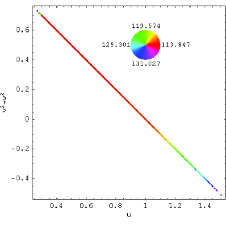
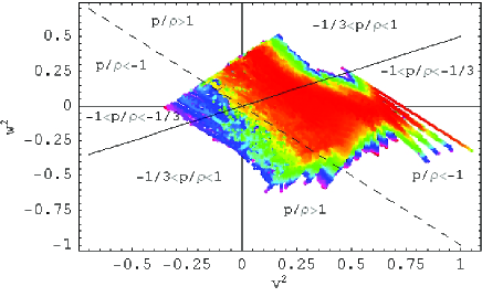
The results presented below were obtained by reconstructing more than $23000$ luminosity-distance curves fitting the data. To show that all the reconstructed curves respect the Friedmann constraint (4), we have depicted in figure 1 a plot of $v^{2}+w^{2}$ versus $u$ for these curves, which as can be seen provides a very good confirmation of the constraint $u+v^{2}+w^{2}=1$. Note that some reconstructions with negative energy density ($v^{2}+w^{2}<0$) are also in agreement with the data, but these correspond to the larger values of $\chi^{2}$. This raises the interesting question of physicality of such solutions. We shall not consider this issue further here, but recall that negative energy densities sometimes arise, for instance in quantum cosmology or in considerations of braneworld models whose bulks possess a negative cosmological constant.

Figure 1: Plot depicting $v^{2}+w^{2}$ versus $u$ for the reconstructed curves. The perfect straight line provides a good confirmation for the constraint $u+v^{2}+w^{2}=1$. The reconstructed points are shaded (coloured: references to colour refer to the web version with colour figures) according to their corresponding $\chi^{2}$ values, with the deepest shade of grey (red), representing the smallest values of $\chi^{2}$.

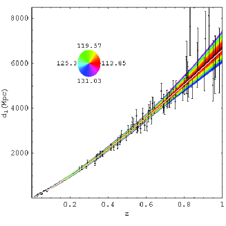
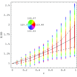
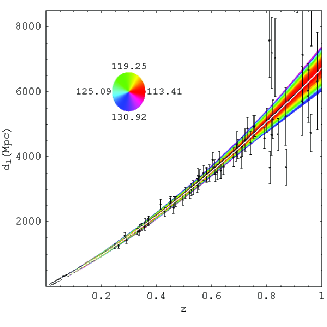
In figure 2 we have plotted the reconstructed luminosity-distance curves (top panel) and the corresponding Hubble parameters (bottom panel) together with their $1\sigma$ confidence levels (dashed lines) respectively. As can be seen from the top panel, the $d_{l}$ curves best fitting the data have a slightly smaller $\chi^{2}$ (with the smallest having $\chi^{2}=113.85$) than the $\Lambda CDM$ model (with $\chi^{2}\sim 114$). Hence, none of the reconstructed models rules out the $\Lambda CDM$ model at $1\sigma$. The difference between our best fitting luminosity-distance curve and that of the $\Lambda CDM$ model becomes noticeable at large redshifts where the former curve is slightly lower. This deviation could come from systematics such as the Malmquist bias. Testing our reconstruction method with several samples of mock data, we obtain curves which very closely agree with the $\Lambda CDM$ model even at large redshifts. However, they are very similar to the curves obtained using the real data. This is due to the fact that the real data are themselves very close to the $\Lambda CDM$ model, despite very small deviations for large redshifts. An example of the luminosity-distance reconstruction with mock data is displayed in figure 3. We do not show the plots for the other physical quantities, including the EOS, since they look very similar to the plots with real data.

We also find the reconstructed Hubble parameters (bottom panel) to have amplitudes which are in qualitative agreement with those found by other authors using different reconstruction techniques Ala03 . Here again, mock data produces similar results.

Figure 2: Plots of the reconstructed luminosity-distance (top panel) and Hubble function (bottom panel) with respect to redshift. The dotted white (solid black) line represents the $\Lambda CDM$ model and the white line, the reconstructed luminosity-distance best fitting the data. For the Hubble function we have, for sake of clarity, plotted the points obtained numerically without joining them.

Figure 3: Plot depicting the reconstruction of the luminosity-distance relations using the mock data.

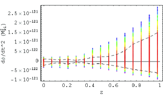
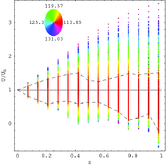
Taking as our theoretical framework GR plus a minimally coupled scalar field, we also reconstructed the kinetic and potential energies corresponding to the scalar field $\phi$, together with their $1\sigma$ confidence levels . These are depicted in figure 4 for the reconstructed $d_{l}$. However, to be able to interpret these reconstructions within the framework of a minimally coupled scalar field, a number of physical constraints need to be taken into account Vik05 , such as those concerning the signs of the potential and kinetic terms. 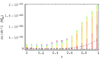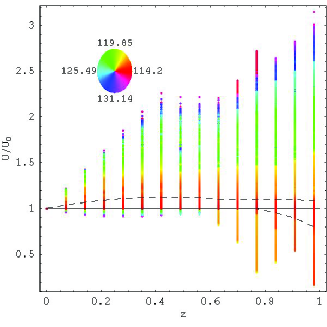To be cautions, we have extracted from the reconstructions the curves corresponding to the quintessence scalar field models with a positive potential. These are depicted in figure 5 showing that the best fitting curves, in the context of quintessence scalar field interpretation, are very close to the $\Lambda CDM$ model. This is particularly striking for $z<0.6$ where the degeneracy is very weak. For larger redshifts, some degeneracy appears due to larger error bars but remains relatively weak.

Figure 4: Plots of all the reconstructed scalar field kinetic (top panel) and potential (bottom panel) energies versus the redshift. The horizontal black lines represent the $\Lambda CDM$ model.

Figure 5: Plots of the reconstructed positive scalar field kinetic (top panel) and positive potential (bottom panel) energies versus the redshift. The horizontal black lines represent the $\Lambda CDM$ model.

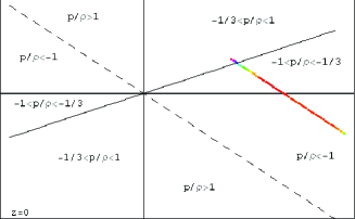
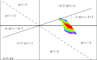
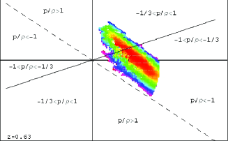
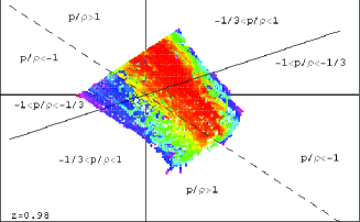
We also reconstructed the dark energy EOS (for all the reconstructed luminosity-distance curves) whose evolution with redshift is depicted in figure 6. To obtain a compact representation of the EOS, we found it more convenient to have a $(v^{2},w^{2})$ plane representation instead of the usual plot of EOS as a function of $z$. This choice of variables is well suited to the particular form (6) of the EOS in this case, whose denominator can take small values (for instance when the kinetic and potential terms take similar values but with different signs) resulting in large variations in the EOS as the redshift increases. As can be seen from figure 6 this allows a compact representation of the EOS, with the diverging values of EOS corresponding to the dashed line. In this figure the horizontal line ($w^{2}=0$) represents the EOS for the cosmological constant ($\mbox{w}_{\phi}=-1$) and the vertical line ($v^{2}=0$) the EOS for a stiff fluid ($\mbox{w}_{\phi}=1$). The remaining line defines the $\mbox{w}_{\phi}=-1/3$ line which demarcates the limit between the accelerated and decelerated expansion.

The shaded (coloured) patches in the panels of figure 6 represent, from top to bottom, the reconstructed values of the EOS at increasing values of the redshift given by $z=0,0.28,0.63,0.98$. Each point constituting the shaded (coloured) patches corresponds to a reconstructed luminosity-distance curve, with the deepest shades of grey (red) representing the best fits (lowest $\chi^{2}$ values). The top panel depicts a cloud of initial points in the $(v^{2},w^{2})$ plane, which since we are initially assuming $u_{0}=\Omega_{m_{0}}=0.27$, are forced to lie on a straight line by the Friedmann constraint $u+v^{2}+w^{2}=1$. As we go to lower panels (higher redshifts), $\Omega_{m}$ evolves differently for each point, resulting in the dispersal of the initial straight line into different clouds of points. Now since we are assuming $d_{l}^{\prime\prime\prime}\leq 0$, $d_{l}^{\prime\prime}$ becomes smaller as the redshift increases, but always stays positive. As a result the initial straight line configuration of points spreads and eventually gets attracted to the neighbourhood of the line $w^{2}=v^{2}+1/3$ which corresponds to $d_{l}^{\prime\prime}=0$. To see this, recall that using (5) and (1) we have $\frac{H}{c}d_{l}^{\prime\prime}=2+\dot{H}H^{-2}$. This together with (4) and (9) then shows that $d_{l}^{\prime\prime}=0$ implies $w^{2}=v^{2}+1/3$. As can be seen from the bottom panel, this line acts as the accumulation end state of the initial cloud of points.

To summarise, the evolution of EOS with $z$ depicted in these panels demonstrates that as $z$ increases, the points corresponding to the $d_{l}$ best fitting the data stay well centred around the cosmological constant line ($w^{2}=0$) in agreement with the behaviour found for the scalar field kinetic and potential energies.

We have also depicted in figure 7 the superposition of panels similar to those depicted in figure 6 for intermediate values of the redshift considered in the range $z\in[0,1]$, in steps of $z=0.07$. We note that some possible variation of dark energy has been reported using reconstruction techniques different from that employed in this paper WanFre04 ; Ala03 ; AlaSah04 . Such variations are also possible according to our results at $1\sigma$ confidence level, but are severely constrained in the context of quintessence scalar field models, as can be seen from Fig. 5.

Figure 6: Figures demonstrating the evolution of the reconstructed EOS (6) versus the redshift in the phase plane $(v^{2},w^{2})$. The top panel, corresponding to redshift $0$, shows the initial points which are forced into a linear configuration due to the choice of $u_{0}=\Omega_{m_{0}}=0.27$ and the constraint equation $u+v^{2}+w^{2}=1$. As the redshift increases (lower panels), the initial straight line configuration of points spreads and eventually gets attracted to the neighbourhood of the line $w^{2}=v^{2}+1/3$ which corresponds to $d_{l}^{\prime\prime}=0$.

Figure 7: Figure showing the superposition of similar panels to figure 6 for all intermediate values of $z\in[0,1]$ in steps of $dz=0.07$. As can be seen the distribution of the points with the deepest shade of grey (red), corresponding to the best fits, is well centred around the cosmological constant line.

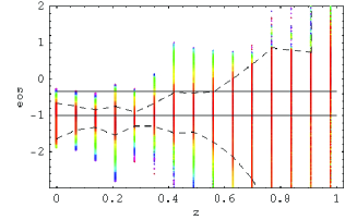
We have also plotted in (top panel of) figure 8 the best fitting reconstructions for the EOS as a function of redshift with the $1\sigma$ confidence level. As can be seen, initially ($z\sim 0$) the EOS takes values around $\sim-1$. Then, around the redshift of $0.45$, the degeneracy increases becoming very large beyond $z=0.8$. This follows the evolution of error bars and noise levels in the data. 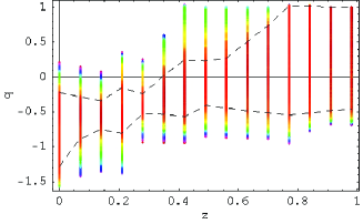We have also plotted the evolution of the associated deceleration parameter (depicted in the bottom panel of the figure 8). 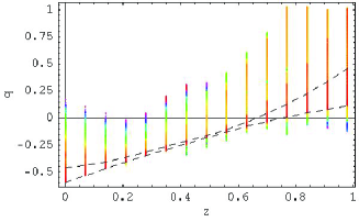This shows that a transition from an accelerated to a decelerated expansion would occur after the redshift of $0.35$. There can, nevertheless, exist solutions which do not undergo such a transition, even at $1\sigma$ confidence level, in agreement with ElgMul06 . This shows that constant as well as negative deceleration parameters are also compatible with the supernovae data, thus indicating that at present the supernova data does not establish with certainty a transition from accelerated to decelerated expansion.

Figure 8: The evolutions of the reconstructed EOS corresponding to the luminosity-distance curves best fitting the data as a function of the redshift (top panel) and the corresponding deceleration parameter (bottom panel) with their $1\sigma$ confidence levels (dashed lines).

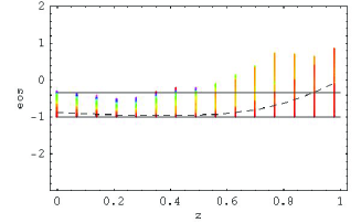
The panels in figure 9 also show the reconstructed EOS and the associated deceleration parameter when the reconstructions were confined to the quintessence scalar field models with positive potentials. As can be seen at $1\sigma$ confidence level, the reconstructed EOS is very close to that of the $\Lambda CDM$ model but could vary weakly beyond $z\simeq 0.6$. Moreover the deceleration can begin for a redshift $z>0.65$.

Figure 9: The evolutions of the reconstructed EOS corresponding to the luminosity-distance curves best fitting the data as a function of the redshift (top panel) and the corresponding deceleration parameter (bottom panel) with their $1\sigma$ confidence levels (dashed lines), using the scalar field representation confined to quintessence models.

IV.2 Constraining $\Omega_{m_{0}}$

Our reconstructions in the previous subsection did not provide any information about the $CDM$ density parameter $\Omega_{m_{0}}$ which was assumed to be $0.27$. This is due to the fact that the luminosity-distance relation is determined purely by the Friedmann equation which is highly degenerate with respect to this parameter. To see this, let us consider a dark energy model with a constant EOS, $\mbox{w}_{\phi}=\Gamma-1$, and the corresponding Friedmann equation

$$(H/H_{0})^{2}=\Omega_{m_{0}}(1+z)^{3}+\Omega_{\phi_{0}}(1+z)^{3\Gamma}$$

Re-writing the $CDM$ density parameter as $\Omega_{m_{0}}=\Omega_{1m_{0}}+\Omega_{2m_{0}}$, the Friedmann equation becomes

$$(H/H_{0})^{2}=\Omega_{1m_{0}}(1+z)^{3}+\Omega_{2m_{0}}(1+z)^{3}+\Omega_{\phi_{0}}(1+z)^{3\Gamma}$$

This form of $H(z)$ may be viewed as a new dark energy model with a different $CDM$ density parameter $\Omega_{1m_{0}}$, and a different dark energy density $\rho_{\phi}$ represented by the last two terms in this expression. Hence without changing the Hubble function we can re-group the last two terms as a new dark energy term thus:

$$(H/H_{0})^{2}=\Omega_{1m_{0}}(1+z)^{3}+\Omega_{1\phi_{0}}\frac{\rho_{\phi}}{\rho_{\phi_{0}}}$$

with a corresponding equation of state given by

$$p_{\phi}/\rho_{\phi}=\frac{\Omega_{2m_{0}}(1+z)^{3}+\Gamma\Omega_{\phi_{0}}(1+z)^{3\Gamma}}{\Omega_{2m_{0}}(1+z)^{3}+\Omega_{\phi_{0}}(1+z)^{3\Gamma}}-1$$

Thus given a Hubble function we can construct different representations with different effective $CDM$ density parameters and dark energy components, but with identical luminosity-distance functions $d_{l}$. This makes transparent the fact that the luminosity-distance $d_{l}$ is potentially highly degenerate with respect to the $CDM$ density in Universe. It also illustrates the fact that a constant EOS can misleadingly become time-dependent if the matter density is incorrectly chosen, as is shown in Sha05 . We should, however, add that since in practice $\Omega_{m_{0}}$ cannot be determined precisely, this demonstrates that a real observer can never prove that $\mbox{w}_{\phi}$ is truly constant, similar to the limitations that exist in determining the exact flatness of the Universe from observations. In practice one can only take the most likely value for $\Omega_{m_{0}}$ given by the most accurate available observations in order to determine the corresponding EOS.

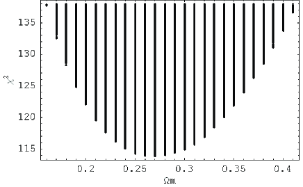
To constrain $\Omega_{m_{0}}$, we need further input from observations. Here we used the recent baryon oscillation data Eis05 (discussed in Section III), to further constrain each luminosity-distance curve. We found that for our reconstructed set of curves $S_{dl}$, $\Omega_{m_{0}}$ lies in the range $0.16<\Omega_{m_{0}}<0.41$, with the best fit obtained for $\Omega_{m_{0}}=0.27$. This can be seen clearly from the plot of $\Omega_{m_{0}}$ versus $\chi^{2}$ shown in figure 10 which justifies the choice of the specific value $\Omega_{m_{0}}=0.27$ in the previous subsection.

Figure 10: Figure depicting the variation of reconstructed $\Omega_{m_{0}}$ with respect to $\chi^{2}$, using the SNLS and BAO data.

IV.3 Robustness of the reconstruction

In this subsection we study the robustness of our results obtained in the previous subsections.

In our reconstructions so far we have used $7$ points ($d_{l},z$) to describe the luminosity-distance curves. This choice was made by trial and error. We find that by taking too many points we can ”over-fit” the data, in the sense that we can always obtain a perfect but artificial match to any set of data. In that case one would in effect be fitting noise with an anomalously low best $\chi^{2}$ which can, among other things, rule out the $\Lambda CDM$ model at $1\sigma$. On the other hand, taking too few points would amount to ”under-fitting” the data. Thus one would not be able to fit the model represented by the data and the best $\chi^{2}$ can be anomalously high. For example, it could make it impossible to fit the $\Lambda CDM$ model. In order to determine the optimal number of points, the use of mock data is extremely useful. We have tested our reconstruction scheme with several sets of mock data, all based on the $\Lambda CDM$ model. Using seven points we were able to recover, in all cases, the $\Lambda CDM$ model at $1\sigma$ with a best $\chi^{2}$ (typically around $113.7$) only a few tenths of percent smaller than $114$ (which is close to the corresponding value for the $\Lambda CDM$ model). This demonstrates that, given the distribution of the SNLS data and the corresponding error bars, our reconstruction process works well (although a slight over-fitting is unavoidable in practice as one is not expected to recover the best fit value exactly). We checked that our results remain robust with small changes in the number of points.

To summarise, care must be taken in choosing the number of points taken to define a luminosity-distance curve. We found that the employment of the mock data together with our conditions (a)-(c) allow an appropriate number of points to be chosen, i.e. around $7$.

We note that the number of points defining a luminosity-distance curve is not related to the degrees of freedom of the underlying theory giving rise to that curve. Thus, a straight line can be defined by $7$ points even though only $2$ points are necessary to construct the line, while analytically the equation of a straight line passing through the origin only has one degree of freedom.

We also checked that reasonable changes in the value of $\Omega_{m_{0}}$ does not alter the qualitative behaviour of dark energy EOS found here.

V Conclusion

We have proposed a model-independent reconstruction scheme which is compatible with current observations and shares a number of geometrical features with the Einstein-de Sitter and $\Lambda CDM$ models, which are the most commonly accepted models representing the early and late dynamics of the Universe. Together these features provide justification for our proposed scheme.

Using this scheme, and assuming $\Omega_{m_{0}}=0.27$ together with the SNLS supernovae data, we have reconstructed a large set of luminosity-distance curves. Using these curves we have reconstructed the cosmological parameters, including the EOS. Our reconstructions show that the luminosity-distance curves best fitting the data correspond to a slightly varying dark energy density with the Universe expanding slightly slower than the $\Lambda CDM$ model. However, the $\Lambda CDM$ model fits the data at $1\sigma$ and the fact that our best fitting luminosity-distance curve is lower than that of the corresponding $\Lambda CDM$ model could be due to systematics such as Malmquist bias. Reconstructing the EOS, large degeneracy appears around $z=0.6$ in agreement with increasing error bars and noise levels in the distribution of data. The reconstructed deceleration parameter shows that the transition redshift to a decelerating Universe should be larger than $z=0.35$.

Assuming the theoretical framework to be GR plus a minimally coupled scalar field, we also considered reconstructions confined to quintessence models with positive potentials. In that case we find the best fitting reconstructed curves to be very close to those corresponding to the $\Lambda CDM$ model, in particular for low redshifts $z<0.6$. For larger redshifts, larger error bars in the data allow a small increase in the kinetic term and EOS and a small decrease in the potential term at $1\sigma$. However, in the context of quintessence interpretation, it seems rather hard to find a model fitting the data better than the $\Lambda CDM$ model at $1\sigma$.

We also used the BAO data to constrain $\Omega_{m_{0}}$ and found that $\Omega_{m_{0}}$ takes values in the range $0.16<\Omega_{m_{0}}<0.41$ with a best fit given by $\Omega_{m_{0}}=0.27$, in close agreement with CMB data Spe03 ; Spe06 .

Using different techniques, and employing supernovae as well as other data, other authors AlaSah04 ; Ala03 ; WanFre04 ; WanMuk04 also find evidence for a possible variation of dark energy density. However, a constant dark energy density is again never ruled out to a satisfactory confidence level and thus the important question of whether the EOS varies in time or not still remains open.

The present paper takes a new step in reconstructing the equation of state by providing a new model-independent reconstruction scheme of the cosmological parameters. Our approach can be applied to other theoretical frameworks which can be cast into GR plus a perfect fluid. It would be interesting to repeat these reconstructions with the next set of SNLS data to determine whether the best fitting curves move closer or further away from the $\Lambda CDM$ model.

References

- [1] A. G. Riess et al., Astro. Phys. J., 607, 665 (2004).
- [2] P. Astier et al., Astron. Astrophys., 447, 31 (2006)
- [3] D.N. Spergel et al., Astrophys. J., 148, 175 (2003).
- [4] D.N. Spergel et al., astro-ph/0603449 (2006).
- [5] M. Tegmark et al., Phys. Rev. D69, 103510 (2004).
- [6] U. Seljak et al., Phys. Rev. D71, 103515 (2005).
- [7] G. Dvali, G. Gabadadze, and M. Porrati, Phys. Lett. B485, 208 (2000).
- [8] S. Fay, Astron. Astrophys., 452, 781 (2006).
- [9] D. J. Eisenstein et al., Astrophys. J., 633, 560 (2005).
- [10] V. Sahni, T. Saini, A. A. Starobinsky, U. Alam, JETP Lett., 77, 201 (2003).
- [11] M. Szydlowski and W. Czaja, Phys. Rev. D69, 023506 (2004).
- [12] O. Elgaroy and T. Multamaki, astro-ph/0603053 (2006).
- [13] U. Alam, V. Sahni, T. Saini, A. A. Starobinsky, MNRAS., 354, 275 (2004).
- [14] A. Vikman, Phys. Rev. D, 71, 023515 (2005).
- [15] U. Alam, V. Sahni, and A. A. Starobinsky, JCAP, 008, 0406 (2004).
- [16] Y. Wang and P. Mukherjee, Astrophys. J., 606, 654 (2004).
- [17] A. Shafieloo, U. Alam, V. Sahni, A. A. Starobinsky, MNRAS, 366, 1081 (2006).
- [18] E. Copeland, A. Liddle and D. Wands, Phys. Rev. D57, 4686 (1998)
- [19] G. Huey and R. Tavakol, Phys. Rev. D65, 043504 (2002).
- [20] Y. Wang and K. Freese, Phys. Lett. B632, 449 (2004).
- [21] R.A. Daly and S.G. Djorgovski, Astrophys. J., 597, 9 (2003).
- [22] R.A. Daly and S.G. Djorgovski, astro-ph/0512576 (2005).