The VLT-FLAMES survey of massive stars:
Mass loss and rotation of early-type stars in the SMC

We have studied the optical spectra of a sample of 31 O- and early B-type stars in the Small Magellanic Cloud, 21 of which are associated with the young massive cluster NGC 346. Stellar parameters are determined using an automated fitting method (Mokiem et al. 2005), which combines the stellar atmosphere code fastwind (Puls et al. 2005) with the genetic algorithm based optimisation routine pikaia (Charbonneau 1995). Comparison with predictions of stellar evolution that account for stellar rotation does not result in a unique age, though most stars are best represented by an age of 1–3 Myr. The automated method allows for a detailed determination of the projected rotational velocities. The present day $v_{\rm r}\sin i$ distribution of the 21 dwarf stars in our sample is consistent with an underlying rotational velocity ($v_{\rm r}$) distribution that can be characterised by a mean velocity of about $160-190\leavevmode\nobreak\ \mbox{km\,s${}^{-1}$}$ and an effective half width of $100-150\leavevmode\nobreak\ \mbox{km\,s${}^{-1}$}$. The $v_{\rm r}$ distribution must include a small percentage of slowly rotating stars. If predictions of the time evolution of the equatorial velocity for massive stars within the environment of the SMC are correct (Maeder & Meynet 2001), the young age of the cluster implies that this underlying distribution is representative for the initial rotational velocity distribution. The location in the Hertzsprung-Russell diagram of the stars showing helium enrichment is in qualitative agreement with evolutionary tracks accounting for rotation, but not for those ignoring $v_{\rm r}$. The mass loss rates of the SMC objects having luminosities of $\log\mbox{$L_{\star}$}/\mbox{$L_{\sun}$}\gtrsim 5.4$ are in excellent agreement with predictions by Vink, de Koter & Lamers (2001). However, for lower luminosity stars the winds are too weak to determine $\dot{M}$ accurately from the optical spectrum. Two of three spectroscopically classified Vz stars from our sample are located close to the theoretical zero age main sequence, as expected. Three additional objects of lower luminosity, which are not given this classification, are also found to lie near the ZAMS. We argue that this is related to a temperature effect inhibiting relatively cool stars from displaying the spectral features characteristic for the Vz luminosity class.

1 Introduction

Mass loss and rotation play a crucial role in the evolution of the most massive stars. These two processes are linked. To illustrate this, fast rotation may lead to an enhanced mass loss, as is, for instance, observed in the case of Be stars (Lamers & Pauldrach, 1991) and $\eta$ Carinae (Smith et al., 2003; van Boekel et al., 2003). Conversely, the stellar winds of these stars will cause loss of angular momentum, leading to spin down. In a Galactic environment the spin down of massive stars is expected to be relatively rapid, essentially “erasing” their initial rotational velocity properties within only a few million years (Meynet & Maeder, 2000). For an environment characteristic of the Small Magellanic Cloud (SMC) it is predicted that the initial conditions of rotational velocity remain preserved during the main sequence life of O-type stars (Maeder & Meynet, 2001), as the strength of stellar winds diminishes with decreasing metal content (e.g. Abbott, 1982; Kudritzki et al., 1987; Vink et al., 2001).

The study of a young SMC cluster containing a substantial population of O-type main sequence stars would allow the role of metallicity on mass loss and angular momentum loss during the early evolution of massive stars to be better constrained. This provides a better insight into the current and perhaps even initial rotational conditions from which this evolution unfolds. Among others, this would provide important constraints on the physics of the formation of massive stars, for instance on the role of magnetic fields and the lifetime of accretion disks (see e.g. Porter & Rivinius, 2003).

The distribution of projected rotational velocities $v_{\rm r}\sin i$ of Galactic early-type stars has been studied by Conti & Ebbets (1977), Penny (1996) and Howarth et al. (1997). The first extragalactic studies of rotational velocities have been presented by Keller (2004) for a sample of Large Magellanic Cloud (LMC) B-type stars in the vicinity of the main sequence turnoff and by Penny et al. (2004) for predominately giant and supergiant SMC and LMC O-type stars. So far, no systematic study for early main sequence O-type stars in a low metallicity environment has been attempted.

The young cluster NGC 346 in the Small Magellanic Cloud (SMC) contains a substantial population of O-type main sequence stars. In the context of the VLT-FLAMES Survey of Massive Stars (Evans et al., 2005), we have used the Fibre Large Array Multi-Element Spectrograph at the ESO Very Large Telescope to obtain spectra of several dozen dwarf O-type stars in this cluster. Our genetic algorithm based fitting method (Mokiem et al., 2005) is used to perform a homogeneous spectroscopic analysis of this set of stars, including the projected rotational velocity as one of the fitting parameters. The $v_{\rm r}\sin i$ information obtained from this analysis may be compared to models of the present and possibly initial (see above) $v_{\rm r}\sin i$ distribution. This is a main aim of this paper.

The strength of radiatively driven winds is predicted to be reduced for decreasing metal content. In the last two decades this prediction has been quantified by different groups who found a metallicity dependence of the mass loss rate of $\mbox{$\dot{M}$}(Z)\propto Z^{0.5-0.7}$ (e.g. Kudritzki et al., 1987; Puls et al., 2000; Vink et al., 2001). Qualitatively this metallicity dependence has been confirmed by several authors (e.g. Puls et al., 1996; Bouret et al., 2003; Evans et al., 2004a; Massey et al., 2005). However, until now a quantitative comparison of the theoretically predicted and the empirically determined $Z$ dependence is still lacking. The analysis of our SMC targets will provide insight in the wind characteristics of objects with a metal content approximately five times lower than in Galactic objects. Consequently, given the large number of objects that we have analysed in a homogeneous way, the current study will for the first time be able to provide such a quantitative comparison.

While comparing mass loss rate predictions with observed values it is important to realise that recent studies of the wind strengths of not too luminous ($\log\mbox{$L_{\star}$}/\mbox{$L_{\sun}$}\lesssim 5.3$) Galactic and SMC dwarf O-type stars (Bouret et al., 2003; Martins et al., 2004, 2005b) seem to indicate that the mass loss rates are significantly (up to two orders of magnitude) lower than expected from theory (Vink, de Koter, & Lamers, 2001). If this is indeed the case it would imply that our chances of actually observing a $v_{\rm r}$ pattern that is representative of the initial distribution will increase, as less angular momentum will be carried away in the stellar wind. However, from the viewpoint of our understanding of the physics of relatively weak stellar winds ($\sim$$10^{-8}$ – $10^{-6}\mbox{$M_{\sun}{\rm yr}^{-1}$}$) the situation is obviously less desirable.

The mass-loss rates reported by Bouret et al. and Martins et al. are based on an analysis of unsaturated ultraviolet resonance lines. The $\dot{M}$ sensitivity that can be obtained using such lines is $\sim$$10^{-9}$ – $10^{-8}\mbox{$M_{\sun}{\rm yr}^{-1}$}$. This is, in principle, much better than is possible using H$\alpha$ as the mass loss diagnostic. Using our automated fitting method and spectra having a signal-to-noise of 50–200 (typical for those secured within the context of our VLT-FLAMES programme) we can push the H$\alpha$ method as low as $\sim$$2\times 10^{-7}\,\mbox{$M_{\sun}{\rm yr}^{-1}$}$. This provides some overlap with the weak wind regime so far reserved for the UV line method. It thus allows for a first investigation of the question whether the so-called “weak wind problem” points to missing physics in the theoretical predictions of mass loss or that there may be problems with the mass loss diagnostic, i.e. that we do not fully understand the formation of UV resonance lines.

The structure of this paper is as follows: in Sect. 2 we describe the data set that has been analysed using our genetic algorithm based fitting method, which is discussed in Sect. 3. The stellar properties of our sample determined in this analysis are presented in Sect. 4. In sections 5, 6 and 7 we investigate and discuss, respectively, the underlying rotational velocity distribution of our sample, the mass loss rates we have determined in the context of weak winds and the evolutionary status of the cluster NGC 346. Sect. 8 summarises and lists the conclusions of our study. Finally, in the appendix the fits and comments on the individual objects are provided.

2 Data description

The sample considered here is mainly drawn from the targets observed in the SMC as part of the VLT-FLAMES survey of massive stars (see Evans et al., 2005). The survey observed two fields in the SMC, centered on the clusters NGC 346 and NGC 330. Here we analyse each of the O-type stars and three luminous B-type stars observed in the NGC 346 field, and two O-type stars from the older NGC 330 cluster.

To improve our sampling of luminosity and temperature within the O-type domain the FLAMES targets were supplemented by eight field stars from the catalogue of Azzopardi & Vigneau (1975, 1982, hereafter AzV, note that in other studies these are also often denoted by AV). These stars were observed using the Ultraviolet and Visual Echelle Spectrograph (UVES) at the VLT as part of the programs 67.D-0238, 70.D-0164 and 074.D-0109 (P.I. Crowther).

Table 1: Basic parameters. Identifications: FLAMES targets (“NGC330” and “NGC346”) from Evans et al. (2006), “MPG” from Massey et al. (1989), “AzV” from Azzopardi & Vigneau (1975, 1982) and “Sk” from Sanduleak (1968). Photometric data for the FLAMES targets is from Momany et al. (2001); for objects with a primary AzV identification these are from Massey (2002) and Massey et al. (2004). Spectral types of the FLAMES targets are from Evans et al. (2006). For convenience previously published spectral types are also given. Sources of these classifications are W77 (Walborn, 1977); NMC (Niemela et al., 1986); G87 (Garmany et al., 1987); MPG (Massey et al., 1989); W00 (Walborn et al., 2000); EH04 (Evans et al., 2004b). Spectral types for the field O-type stars were taken from the catalogues of Garmany et al. (1987) and Walborn et al. (2002). Wind velocities given without brackets are from Garmany & Fitzpatrick (1988); Haser et al. (1998); Prinja & Crowther (1998); Crowther et al. (2002); Bouret et al. (2003); Evans et al. (2004a, c); Massey et al. (2004). Values between brackets are calculated from the escape velocity at the stellar surface.

Primary ID	Cross-IDs			Spectral	Published	$V$	$A_{V}$	$M_{V}$	$v_{\infty}$
	MPG	AzV	Sk	Type	ST				[km s-1]
NGC 346-001a)	MPG 789	AzV 232	Sk 80	O7 Iaf+	O7 Iaf+ [W77]	12.31	0.40	$-6.99$	1330
					O7 If [MPG]
NGC 346-007a)	MPG 324	…	…	O4 V((f+))	O4-5 V [NMC]	14.07	0.12	$-4.95$	2300
					O4 V((f)) [MPG]
					O4 ((f)) [W00]
NGC 346-010	…	AzV 226	…	O7 IIIn((f))	O7 III [G87]	14.37	0.31	$-4.84$	[1832]
NGC 346-012	…	AzV 202	…	B1 Ib	B1 III [G87]	14.39	0.09	$-4.60$	[1568]
NGC 346-018	MPG 217	…	…	O9.5 IIIe	…	14.78	0.56	$-4.68$	[1481]
NGC 346-022	MPG 682	…	…	O9 V	O8 V [MPG]	14.91	0.16	$-4.14$	[3305]
NGC 346-025a)	MPG 848	…	…	O9 V	O8.5 V [MPG]	14.95	0.12	$-4.07$	[2816]
NGC 346-026	MPG 12	…	…	B0 IV	O9.5 V [MPG]	14.98	0.50	$-4.42$	[2210]
					O9.5-B0 V (N str) [W00]
					O9.5 III [EH04]
NGC 346-028	MPG 113	…	…	OC6 Vz	O6 V [MPG]	15.01	0.19	$-4.08$	[2369]
					OC6 Vz [W00]b)
NGC 346-031	…	…	…	O8 Vz	…	15.02	0.16	$-4.04$	[2461]
NGC 346-033	MPG 593	…	…	O8 V	…	15.07	0.19	$-4.02$	[4102]
NGC 346-046	…	…	…	O7 Vn	…	15.44	0.12	$-3.58$	[2723]
NGC 346-050	MPG 299	…	…	O8 Vn	O9 V [MPG]	15.50	0.03	$-3.43$	[2661]
NGC 346-051	MPG 523	…	…	O7 Vz	O7 V+neb [MPG]	15.51	0.16	$-3.54$	[3233]
NGC 346-066	MPG 213	…	…	O9.5 V	…	15.75	0.16	$-3.30$	[2931]
NGC 346-077	MPG 238	…	…	O9 V	B0: [MPG]	15.88	0.40	$-3.42$	[2205]
NGC 346-090	…	…	…	O9.5 V	…	15.96	0.37	$-3.31$	[2978]
NGC 346-093	MPG 304	…	…	B0 V	…	16.01	0.34	$-3.23$	[3516]
NGC 346-097	MPG 519	…	…	O9 V	…	16.06	0.74	$-3.58$	[4004]
NGC 346-107	MPG 559	…	…	O9.5 V	…	16.20	0.09	$-2.79$	[2547]
NGC 346-112	MPG 327	…	…	O9.5 V	…	16.24	0.19	$-2.85$	[2368]
NGC 330-013	…	AzV 186	…	O8.5 II-III((f))	O7 III [G87]	14.00	0.56	$-5.46$	1600
					O8 III((f)) [EH04]
NGC 330-052	…	…	…	O8.5 Vn	O8 V [EH04]	15.69	0.16	$-3.36$	[2005]
AzV 14	…	…	Sk 9	O5 V	…	13.55	0.47	$-5.81$	2000
AzV 15	…	…	Sk 10	O7 II	…	13.12	0.40	$-6.18$	2125
AzV 26	…	…	Sk 18	O7 III	…	12.46	0.47	$-6.90$	2150
AzV 95	…	…	…	O7 III	…	13.78	0.43	$-5.55$	1700
AzV 243	…	…	Sk 84	O6 V	…	13.84	0.47	$-5.53$	2125
AzV 372	…	…	Sk 116	O9 Iabw	…	12.59	0.50	$-6.81$	1550
AzV 388	…	…	…	O4 V	…	14.09	0.34	$-5.15$	1935
AzV 469	…	…	Sk 148	O8.5 II((f))	…	13.12	0.47	$-6.25$	1550

^a) binary; ^b) the source of the type adopted here

Table 1 lists some of the basic observational properties of the programme stars analysed together with common aliases used in other studies. For a full description of the observational properties of the FLAMES targets see Evans et al. (2006). Note that five of these objects and six of the field stars were recently also analysed using line blanketed stellar atmosphere models (Crowther et al., 2002; Bouret et al., 2003; Evans et al., 2004a; Massey et al., 2004; Heap et al., 2006). A comparison with our findings is presented in the appendix. Each of the FLAMES targets were observed with the Giraffe spectrograph at least six times, at each of six wavelength settings. The effective resolving power of the observations is $R\simeq 20\,000$, full details are given by Evans et al. (2006). The multiple exposures, often at different epochs, allowed for the detection of variable radial velocities, with a number of binaries detected (see Evans et al., 2006). Three of the stars analysed here are detected as binaries (NGC 346-001 & NGC 346-025) or are found to have variable velocities suggestive of binarity (NGC 346-007), as noted in Table 1. Note that none of these appear to have massive companions, which could have a significant effect on the derived parameters if they were present.

A general description of the reduction of the FLAMES data was given by Evans et al. (2005). The most pertinent part of the reductions for the current study is that of sky subtraction. A master sky-spectrum was created from combining the sky fibres (typically 15), individually scaled by their relative fibre throughput. In general the sky background is low for our (relatively bright) targets, and this approach successfully removes the background contribution. However, in regions such as NGC 346 which has strong nebular emission, accurate subtraction of nebular features in multi-fibre data is notoriously difficult. This does not hamper our analysis, except in the core of the H$\alpha$ Balmer line. For most stars the core nebular emission is well-resolved and we simply only consider the wings of the profile in the automated line fits. Tests assessing the impact of possible residual nebular contamination in the line wings or over-subtraction of sky components are discussed in Sect. 3.3.

For each wavelength range the individual sky-subtracted spectra were co-added, then normalised using a cubic-spline fit to the continuum. These normalised data were finally merged to obtain a final spectrum covering 3850–4750 and 6300–6700 Å. The combined spectra have a typical signal-to-noise ratio of 50–200, depending on the magnitude of the target.

Spectral types for the field O-type stars were taken from the catalogues of Garmany et al. (1987) and Walborn et al. (2002). The FLAMES spectra were classified by visual inspection, using published standards, in particular the atlas of Walborn & Fitzpatrick (1990), with consideration to the lower metallicity environment of the SMC (e.g. Walborn et al., 2000). The classifications quoted in Table 1 are from Evans et al. (2006).

The majority of the field stars were observed with the VLT-UVES spectrograph during a visitor run on 27-28 September 2001 under program 67.D-0238. UVES is a two arm cross-dispersed echelle spectrograph, the red arm of which contains a mosaic of two detectors. A standard blue setting, with central wavelength 437 nm provided continuous coverage between 3730–5000 Å, recorded on a single 2$\times 4$K EEV CCD. A non-standard red setting with central wavelength 830 nm included an identical EEV CCD covered 6370–8313 Å, whilst a 2$\times$4K MIT-LL CCD covered 8290–10250 Å. A 1^′′ slit was used in variable seeing conditions to provide a spectral resolution of 0.09 Å at H$\alpha$. Exposure times ranged from 1200 to 3000 seconds.

Subsequently, AzV 388 was observed with UVES on 5 Dec. 2002 under service program 70.D-0164, using a standard setup with central wavelength 390 nm (blue, 3300–4500 Å) and 564 nm (red, 4620–5600 and 5675–6650 Å), plus a second red setup with central wavelength 520 nm (4170–5160 and 5230–6210 Å). The exposure time was 2700 s for each setup, with a 1.2^′′ slit. Finally, AzV 95 was observed with UVES under service program 074.D-0109 on Nov. 27 2004, using standard setups with central wavelengths 390/564 nm and 437/860 nm, with individual 2200 s exposures, again with a 1.2^′′ slit. In all cases, the two-dimensional CCD frames were transformed to extracted one-dimensional spectra using the UVES pipeline software. The S/N in individual blue spectra ranged from $\sim$50 to $\sim$120.

The quoted photometry for the FLAMES targets in the NGC 346 and NGC 330 fields is taken from the ESO Imaging Survey (EIS) pre-FLAMES release by Momany et al. (2001). These data compare well to the values obtained previously by Massey et al. (1989) and Azzopardi & Vigneau (1975, 1982), with an average difference of 0.04 magn for both $V$ and $(B-V)$ and incidental (two cases) maximum differences of approximately 0.1 magn. Photometric data for the field stars was taken from the UBVR CCD survey of Massey (2002) and Massey et al. (2004).

The interstellar extinction ($A_{V}$) listed in Table 1 was calculated using intrinsic colours from Johnson (1966, and references therein) and by assuming a ratio of total to selective extinction of $\mbox{$R_{V}$}=3.1$. Using these $A_{V}$ values, extinction corrected visual magnitudes ($V_{0}$) were calculated from the observed $V$-band magnitudes. Finally, the absolute visual magnitude $M_{V}$, was calculated taking a distance modulus of 18.9 magn (Westerlund, 1997; Harries et al., 2003; Hilditch et al., 2005).

3 Analysis method

To analyse the large number of spectra we use an automated fitting method. This method was developed by Mokiem et al. (2005, hereafter Paper I) for the fitting of the profiles of hydrogen and helium lines and provides a means for an unbiased and homogeneous analysis of large samples of early-type stars. For a detailed description we refer to this paper. Here we will only give a brief description of the method and modifications of its implementation.

The automated fitting method consists of two main components. The first component is the stellar atmosphere code fastwind of Puls et al. (2005). This fast performance code incorporates non-LTE and line blanketing following the concept of a unified model atmosphere to synthesise hydrogen and helium line profiles. To optimise the input parameters for fastwind, i.e. to determine the fit parameters for a certain spectrum, the genetic algorithm based optimisation routine pikaia (Charbonneau, 1995) is used. This second component is capable of global optimisation and in combination with fastwind provides, as was shown in Paper I, a robust method for the fitting of the hydrogen and helium spectra for a broad range of O- and early B-type stars.

In short the automated method determines the best fit by calculating consecutive generations of fastwind models. In every generation the models which fit the observed spectrum the best are selected and their parameters are crossbred and mutated to create new sets of parameters. Using these sets a new generation of models is calculated. The procedure is repeated until the fit quality of the best-fitting model is maximised. This fit quality is defined as the inverted sum of the reduced chi squared, $\chi_{\rm red}^{2}$, values of the observed hydrogen and helium line profiles and the synthetic line profiles. In this sum each spectral line has a weight assigned. These weights are used to express the accuracy with which the model atmosphere code is believed to be able to reproduce certain lines. For instance, the He i line at 4471 Å is given a low weight for late type supergiants because of complications due to the so-called “generalised dilution effect” (Voels et al., 1989) from which this line suffers. A lower weight is assigned to the neutral helium singlet lines for early and mid-type because the codes fastwind and cmfgen (Hillier & Miller, 1998) show a discrepancy in the predictions of these diagnostics (Puls et al., 2005). In Paper I the full weighting scheme is described and discussed.

Table 2: Results of the formal tests. Input parameters of the formal test models are given in the “In” column and parameters obtained with the automated fitting method by fitting synthetic data created from these models are listed in the “Out” column. The results were obtained by evolving a population of 72 fastwind models over a course of 200 generations.

	Set A	Search		Set B	Search		Set C	Search
	In	range	Out	In	range	Out	In	range	Out
Spectral type	O3 I			O5.5 I			O9.5 V
$T_{\rm eff}$ [kK]	47.0	[44, 50]	46.9	40.0	[37, 43]	39.6	33.0	[29, 35]	33.0
$\log{{g}}$ [cm s-2]	3.80	[3.4, 4.1]	3.82	3.6	[3.3, 4.0]	3.57	4.00	[3.6, 4.3]	3.97
$R_{\star}$ [$R_{\sun}$]	18.0		$-$	20.0		$-$	8.0		$-$
$\log\mbox{$L_{\star}$}$ [$L_{\sun}$]	6.17		$-$	5.96		$-$	4.83		$-$
$v_{\rm turb}$ [km s-1]	5.0	[0, 20]	8.01	15.0	[0, 20]	12.1	10.0	[0, 20]	14.5
$Y_{\rm He}$	0.15	[0.05, 0.30]	0.16	0.10	[0.05, 0.30]	0.10	0.10	[0.05, 0.30]	0.09
$v_{\rm r}\sin i$ [km s-1]	200	[100, 300]	194	250	[100, 300]	243	300	[200, 400]	302
$\dot{M}$ [$10^{-6}$$M_{\sun}{\rm yr}^{-1}$]	2.9	[0.2, 8.0]	3.2	1.9	[0.1, 5.0]	1.5	0.022	[0.001, 0.1]	0.031
$\beta$	1.20	[0.5, 1.5]	1.15	1.0	[0.5, 1.5]	1.04	0.80	[0.5, 1.5]	0.98
$v_{\infty}$ [km s-1]	3000		$-$	2200		$-$	2000		$-$

3.1 Fit parameters

For the fitting of the spectra we allow for seven free parameters. These parameters are the effective temperature $T_{\rm eff}$, the surface gravity $g$, the helium over hydrogen number density $Y_{\rm He}$, the microturbulent velocity $v_{\rm turb}$, the projected rotational velocity $v_{\rm r}\sin i$, the mass loss rate $\dot{M}$ and the exponent of the beta-type velocity law describing the supersonic wind regime of the stellar atmosphere. In contrast to Paper I, $v_{\rm r}\sin i$ is now treated as a free parameter. This could be done because the FLAMES spectra are of sufficiently high resolution to allow for a self consistent determination of this parameter (see Sect. 3.2). Note that this parameter can also be determined relatively accurately using alternative methods (see Sect. 4.7). The reason that we still incorporate it as a free parameter is that it allows for a meaningful estimate of the error in this parameter. More importantly, it allows for the propagation of this uncertainty in the error estimates of the other fit parameters.

An important parameter which cannot be determined from the optical spectra of O stars is the terminal velocity of the wind $v_{\infty}$. Therefore, if a value obtained from the analysis of ultraviolet (UV) wind lines is available for a certain object, we keep $v_{\infty}$ fixed at that value. If no $v_{\infty}$ determination is available, the scaling relation of $v_{\infty}$ with the escape velocity at the stellar surface ($v_{\rm esc}$) is used throughout the fitting process. For early-type stars this scaling implies that the ratio $\mbox{$v_{\infty}$}/\mbox{$v_{\rm esc}$}=2.6$ is adopted (Lamers et al., 1995). In some cases this produced relatively large wind velocities (see Tab. 1). However, these individual cases do not have a significant impact on our results, as for most of these objects we could only derive upper limits for the mass loss rate (also see Sect. 4.6).

As the current implementation of the fitting method only analyses the hydrogen and helium lines, no explicit abundance values other than the ratio of these two elements can be determined. Therefore, we adopted fixed values for the atmospheric abundances of the background metals. For these values we use the Solar abundances from Grevesse & Sauval (1998, and references therein) scaled proportionally with respect to mass ratios by the same factor for all elements heavier than helium. Iron, due to its strong line blanketing effect on the stellar atmosphere and emergent spectrum, can be considered to be the most important metal element. Large differences between the abundances of other metals, such as nitrogen, have been reported for the Galaxy and SMC (e.g. Trundle et al., 2004), although their effect upon the spectroscopic analysis of the hydrogen and helium lines are negligible. Consequently, we set the metallicity scaling factor equal to the iron abundance ratio of the SMC. From the analysis of early type SMC stars this ratio is found to be 1/5 times Solar (Rolleston et al., 2003).

3.2 Formal tests

As argued in Paper I so-called formal tests, i.e. fitting of synthetic data, are an integral part of the automated fitting method. First of all such tests are necessary to assess whether the data quality is sufficient to secure a successful determination of the global optimum in parameter space, i.e. whether it will recover the global best fit. Secondly, they are necessary to estimate the minimum number of generations that have to be calculated in order to find this best fit. Consequently, by fitting synthetic data with a similar quality as our observed spectra, we can establish the minimum number of generations that have to be calculated to safeguard that the best possible fit will be obtained when fitting the real spectra.

Similar to Paper I three data sets were created based on fastwind models with parameters representing different types of early-type stars. For these three data sets, which are denoted by A, B and C, the input parameters of the fastwind models are listed in Tab. 2. Set A and set B correspond to bright hot supergiants. The parameters in set C represent a cooler dwarf O-type star. For the mass loss rates we adopted values based on the prediction of Vink et al. (2001) assuming $Z_{\rm SMC}=0.2\,\mbox{$Z_{\sun}$}$.

Using the line profiles from the fastwind models the synthetic data was created by first convolving the profiles with a rotational broadening profile. To the broadened profiles Gaussian distributed noise corresponding to a signal-to-noise ratio of 50, was added. This value approximately corresponds to the lowest S/N in our sample. Finally, as nebular emission requires us to ignore the cores of hydrogen and neutral helium lines in the fitting of our target stars, we also removed these cores from our test data set. In case of the He i lines 2 Å from the central core was cut out. From the hydrogen lines, with exception of H$\alpha$, 3 Å was removed. Of all observed line profiles H$\alpha$ exhibits the strongest nebular contamination. Therefore, a larger region of 5 Å was removed from its core.

The lines from the FLAMES data that will be fitted are the hydrogen Balmer lines H$\alpha$  H$\gamma$ and H$\delta$; the He i singlet line at 4387 Å; the He i triplet lines at 4026, 4471 and 4713 Å, where the first line is actually a blend with He ii; and the He ii lines at 4200, 4541 and 4686 Å. In the formal test we also fit this set of lines. Table 2 lists, for the above set of lines for the different data sets the final fit parameters obtained by evolving a population of 72 fastwind models over a course of 200 generations. Also listed in Tab. 2 are the parameter ranges for each parameter in which the fitting method was allowed to search for the best fit.

For all three tests the automated method was able to find the global optimum. There are some differences between the final fit parameters and the input parameters. However, these can be explained by the low quality of the data simulated and the fact that the sensitivity of some parameters becomes less in certain parts of parameter space. The latter explains the difference between the wind parameters found in case of data set C. As the wind of this object is very weak (order $10^{-8}$ $M_{\sun}{\rm yr}^{-1}$) very little information about it is available in the spectrum. Consequently, the fit parameters describing the wind ($\beta$, $\dot{M}$) are relatively poorly constrained, with the errors in $\dot{M}$ becoming as large as the actual $\dot{M}$ value.

The low S/N also decreases the sensitivity of the fit parameters. For decreasing S/N the global optimum in parameter space becomes shallower. Consequently, the error on the fit parameters increases, as these are a measure of the width of this optimum (see Paper I). This explains the differences in the microturbulent velocities ($\sim$45%), as well as the mass loss rate found for data set B.

To locate the best fit, respectively, approximately 100, 50 and 60 generations were needed in case of data set A, B and C. To obtain robust results we adopt 150 generations as the minimum value in fitting our programme stars.

3.3 Nebular emission

The subtraction of nebular emission features in multi-fibre data can be problematic. The use of a combined sky-spectrum, for instance, does not always result in a complete removal of the nebular component and in other cases may result in an over-subtraction of nebular features. To best cope with these potential problems in the automated fitting method we only consider the wings of the line profiles, ignoring any core nebular contamination. As in most cases the core nebular feature is well resolved (also see Evans et al., 2005) and as the removal of the line cores does not hamper an accurate determination of the fit parameters (see Sect. 3.2), this approach seems justified. It is much more difficult to assess the extent to which the determination of the fundamental parameters might be influenced by residual nebular contamination or subtraction effects in the line wings. Here we can only perform limited tests. To assess the effect of too much sky-subtraction we looked in more detail to the non-sky-subtracted data for NGC 346-010 and NGC 346-077.

To determine if the derived mass loss rates are affected by over-subtraction of nebular features in the H$\alpha$ Balmer line, we refitted the non-sky-subtracted spectrum of the O7 giant NGC 346-010. From the targets observed with FLAMES this object has the smallest mass loss rate that we could determine accurately, i.e. with error estimates smaller than 0.2 dex. Therefore, if incorrect sky-subtractions would be an issue, the mass loss rate estimate of this object would be affected the most. In comparison with the fit parameters determined from the sky-subtracted spectrum, no significant differences are found for any of the parameters obtained from the non-sky-subtracted spectrum. In more detail, the mass loss derived from the non-sky-subtracted spectrum is found to be larger by the small amount of $\sim$0.07 dex, and can be attributed to the slightly larger $\log{{g}}$ ($\sim$0.08 dex). As no UV spectrum is available for this object, $v_{\infty}$ was scaled with $v_{\rm esc}$, resulting in an approximately ten percent higher terminal flow velocity. As $\dot{M}$ is connected to $v_{\infty}$ through the continuity equation, this explains the 0.07 dex increase in the mass loss rate.

The second test we performed was on the spectrum of the O9 dwarf NGC 346-077. This relatively faint object suffers from quite severe nebular contamination in its line profiles. We find that the fit parameters obtained from the non-sky-subtracted spectrum compare well with the values determined from the sky-subtracted spectrum. Within the error bars the two parameter sets, again, are in agreement. Only a relatively large difference is found for the microturbulent velocity. This parameter was found to be reduced by $\sim$14 km s^-1 in the fit of the non-sky-subtracted spectrum. However, we do not attribute this relatively large change to issues due to nebular contamination. Instead, as the formal tests have shown, an accurate determination of this parameter is notoriously difficult for low signal to noise spectra (see also Sect. 4.5).

Now, what if our combined sky-spectrum underestimates the real sky background in the line wings? To assess this, ideally one would like to compare the current fitting results to results obtained from data with a local sky-subtraction. For NGC 346-001 we had the opportunity to perform such a test, as also the spectrum analysed by Crowther et al. (2002) was available. A fit of this spectrum resulted in parameters nearly identical to those obtained from the VLT-FLAMES spectrum. In particular the wind parameters $\beta$ and $\dot{M}$, which are expected to be the most sensitive to nebular contamination, were found to agree within, respectively, 10 percent and 0.03 dex. In itself, this agreement is reassuring, though, we note that NGC 346-001 is located away from the cluster centre (see Evans et al., 2006). Consequently, other objects might still suffer more from nebular contamination. With respect to the mass loss rate determinations, we note that from the objects in NGC 346 only four have a reliable mass loss rate. Out of these only one object (NGC 346-033) lies close to the core of the cluster. Therefore, its mass loss may be more uncertain than is suggested by the formal errors (also see Sect. 4.6). The other three objects (NGC 346-001, -010 and -012) lie at relatively large distances from the core, where we anticipate the background contribution to be relatively small.

Table 3: Fundamental parameters determined using GA optimised spectral fits, with $T_{\rm eff}$ in kK, $\log{{g}}$ and $\log{{g}}_{\rm c}$ in cm s^-2, $R_{\star}$ in $R_{\sun}$, $L_{\star}$ in $L_{\sun}$, $v_{\rm turb}$ and $v_{\rm r}\sin i$ in km s^-1, $\dot{M}$ in $M_{\sun}{\rm yr}^{-1}$, $M_{\rm s}$ and $M_{\rm ev}$ in $M_{\sun}$ and $Q_{0}$ in number of photons per second. Results were obtained using a population of 72 fastwind models evolved over a minimum of 150 generations. Gravities corrected for centrifugal acceleration ($\log{{g}}_{\rm c}$) were used to calculate the spectroscopic masses ($M_{\rm s}$). Evolutionary masses ($M_{\rm ev}$) were derived from the tracks of Charbonnel et al. (1993). Note that “NGC” is omitted from the identifications of the FLAMES targets.

ID	ST	$T_{\rm eff}$	$\log{{g}}$	$\log{{g}}_{\rm c}$	$R_{\star}$	$\log\mbox{$L_{\star}$}$	$Y_{\rm He}$	$v_{\rm turb}$	$v_{\rm r}\sin i$	$\dot{M}$	$\beta$	$M_{\rm s}$	$M_{\rm ev}$	$\log\mbox{$Q_{0}$}$
346-001	O7 Iaf+	34.1	3.35	3.36	29.3	6.02	0.24	20.0	74	6.04$\cdot 10^{-6}$	1.15	71.5	65.5	49.60
346-007	O4 V((f+))	42.8	3.95	3.95	9.7	5.45	0.08	12.0	105	2.30$\cdot 10^{-7}$	0.80	30.9	39.2	49.16
346-010	O7 IIIn((f))	35.9	3.54	3.69	10.2	5.20	0.12	19.6	313	6.02$\cdot 10^{-7}$	0.80	18.6	27.4	48.76
346-012	B1 Ib	26.3	3.35	3.35	12.1	4.80	0.07	11.1	29	1.24$\cdot 10^{-8}$	0.74	12.0	16.6	46.75
346-018	O9.5 IIIe	32.7	3.33	3.37	11.1	5.10	0.10	0.0	138	9.65$\cdot 10^{-8}$	0.80	10.6	23.6	48.55
346-022	O9 V	36.8	4.20	4.20	7.3	4.95	0.09	8.6	55	1.06$\cdot 10^{-7}$	0.80	31.3	23.5	48.37
346-025	O9 V	36.2	4.07	4.08	7.2	4.90	0.10	6.3	138	1.25$\cdot 10^{-7}$	0.80	23.0	22.6	48.31
346-026	B0 IV	32.6	3.76	3.76	9.2	4.93	0.11	10.6	67	5.25$\cdot 10^{-8}$	0.80	17.7	20.7	48.06
346-028	OC6 Vz	42.9	3.97	3.97	6.5	5.10	0.16	10.3	27	1.00$\cdot 10^{-7}$	0.80	14.3	31.9	48.81
346-031	O8 Vz	39.5	3.99	3.99	6.7	4.99	0.16	3.9	18	5.71$\cdot 10^{-8}$	0.80	15.8	26.7	48.60
346-033	O8 V	39.9	4.44	4.45	6.6	4.99	0.07	17.5	188	7.42$\cdot 10^{-7}$	0.80	44.2	27.1	48.54
346-046	O7 Vn	39.7	4.17	4.25	5.4	4.81	0.12	13.2	340	1.01$\cdot 10^{-7}$	0.80	18.7	24.0	48.39
346-050	O8 Vn	37.2	4.16	4.25	5.2	4.67	0.13	10.2	357	7.30$\cdot 10^{-8}$	0.80	17.9	20.6	48.12
346-051	O7 Vz	41.6	4.33	4.33	5.2	4.87	0.10	6.8	18	1.73$\cdot 10^{-7}$	0.80	21.5	26.5	48.50
346-066	O9.5 V	35.6	4.25	4.26	5.2	4.59	0.09	16.4	129	9.75$\cdot 10^{-8}$	0.80	18.0	18.9	47.88
346-077	O9 V	36.5	3.99	4.03	5.3	4.65	0.09	14.6	177	7.22$\cdot 10^{-8}$	0.80	10.8	19.9	48.09
346-090	O9.5 V	34.9	4.26	4.28	5.3	4.56	0.09	11.3	188	9.82$\cdot 10^{-8}$	0.80	19.4	18.3	47.76
346-093	B0 V	34.4	4.42	4.43	5.2	4.53	0.09	11.2	187	1.49$\cdot 10^{-7}$	0.80	26.3	17.8	47.60
346-097	O9 V	37.5	4.49	4.49	5.6	4.75	0.08	8.5	22	2.03$\cdot 10^{-7}$	0.80	35.5	21.7	48.14
346-107	O9.5 V	35.9	4.23	4.23	4.1	4.40	0.09	5.0	55	4.06$\cdot 10^{-8}$	0.80	10.4	17.9	47.73
346-112	O9.5 V	34.4	4.15	4.17	4.3	4.36	0.10	15.6	143	2.44$\cdot 10^{-8}$	0.80	9.8	16.6	47.53
330-013	O8.5 II-III((f))	34.5	3.40	3.41	14.1	5.40	0.18	19.1	73	2.96$\cdot 10^{-7}$	1.55	18.6	32.2	48.92
330-052	O8.5 Vn	35.7	3.91	4.02	5.2	4.60	0.16	11.3	291	3.66$\cdot 10^{-8}$	0.80	10.5	19.0	48.00
AzV 14	O5 V	45.3	4.10	4.11	13.9	5.86	0.10	18.2	212	2.67$\cdot 10^{-7}$	0.80	90.9	61.7	49.60
AzV 15	O7 II	39.4	3.69	3.70	18.3	5.82	0.10	2.9	135	1.12$\cdot 10^{-6}$	1.12	60.9	53.9	49.53
AzV 26	O7 III	40.1	3.75	3.75	25.2	6.17	0.09	0.9	128	1.71$\cdot 10^{-6}$	1.17	132.0	85.7	49.86
AzV 95	O7 III	38.2	3.66	3.66	13.8	5.56	0.13	13.2	68	3.56$\cdot 10^{-7}$	1.16	32.1	39.3	49.19
AzV 243	O6 V	42.6	3.94	3.94	12.8	5.68	0.12	0.0	59	2.64$\cdot 10^{-7}$	1.37	52.4	49.0	49.39
AzV 372	O9 Iabw	31.0	3.19	3.22	28.7	5.83	0.11	20.0	135	2.04$\cdot 10^{-6}$	1.28	49.3	49.8	49.23
AzV 388	O4 V	43.3	3.95	3.96	10.6	5.55	0.09	13.2	163	3.34$\cdot 10^{-7}$	0.80	37.5	43.4	49.27
AzV 469	O8.5 II((f))	34.0	3.41	3.42	20.6	5.70	0.17	19.8	81	1.10$\cdot 10^{-6}$	1.16	40.5	43.6	49.20

A value of $\beta=0.80$ corresponds to an assumed fixed value

Table 4: Optimum width based error estimates for the seven fit parameters. The ND entries correspond to error in $v_{\rm turb}$ that reach up to the maximum allowed value of $v_{\rm turb}$ and, therefore, are formally not defined. See text for details on the calculation of the uncertainties in the derived parameters. Units: $T_{\rm eff}$ in kK, $\log{{g}}$ and $\log{{g}}_{\rm c}$ in cm s^-2, $R_{\star}$ in $R_{\sun}$, $L_{\star}$ in $L_{\sun}$, $v_{\rm turb}$ and $v_{\rm r}\sin i$ in km s^-1, $\dot{M}$ in $M_{\sun}{\rm yr}^{-1}$, $M_{\rm s}$ and $M_{\rm ev}$ in $M_{\sun}$ and $Q_{0}$ in number of photons per second. Note that “NGC” is omitted from the identifications of the FLAMES targets.

ID

$\Delta$$T_{\rm eff}$

$\Delta$$\log{{g}}_{\rm c}$

$\Delta$$R_{\star}$

$\Delta\log\mbox{$L_{\star}$}$

$\Delta$$Y_{\rm He}$

$\Delta$$v_{\rm turb}$

$\Delta$$v_{\rm r}\sin i$

$\log\Delta$$\dot{M}$

$\Delta$$\beta$

$\Delta$$M_{\rm s}$

$\Delta$$M_{\rm ev}$

$\Delta\log\mbox{$Q_{0}$}$

346-001

${}^{-0.6}_{+0.6}$

${}^{-0.12}_{+0.17}$

$\pm$2.0

$\pm$0.06

${}^{-0.03}_{+0.06}$

${}^{-2.8}_{\rm+ND}$

${}^{-9}_{+15}$

${}^{-0.04}_{+0.05}$

${}^{-0.09}_{+0.06}$

${}^{-19}_{+35}$

${}^{-6}_{+6}$

${}^{-0.17}_{+0.16}$

346-007

${}^{-0.7}_{+1.5}$

${}^{-0.04}_{+0.08}$

$\pm$0.7

$\pm$0.08

${}^{-0.01}_{+0.01}$

${}^{-8.7}_{+4.7}$

${}^{-13}_{+10}$

${}^{-1.30}_{+0.23}$

$-$

${}^{-4}_{+8}$

${}^{-3}_{+5}$

${}^{-0.12}_{+0.20}$

346-010

${}^{-1.0}_{+1.3}$

${}^{-0.08}_{+0.13}$

$\pm$0.7

$\pm$0.09

${}^{-0.03}_{+0.04}$

${}^{-7.6}_{\rm+ND}$

${}^{-23}_{+27}$

${}^{-0.14}_{+0.09}$

$-$

${}^{-3}_{+6}$

${}^{-3}_{+3}$

${}^{-0.23}_{+0.30}$

346-012

${}^{-0.5}_{+0.8}$

${}^{-0.05}_{+0.10}$

$\pm$0.8

$\pm$0.08

${}^{-0.01}_{+0.01}$

${}^{-1.3}_{+1.9}$

${}^{-4}_{+4}$

${}^{-0.20}_{+0.52}$

${}^{-0.03}_{+0.41}$

${}^{-2}_{+4}$

${}^{-1}_{+1}$

${}^{-0.15}_{+0.20}$

346-018

${}^{-1.3}_{+1.1}$

${}^{-0.14}_{+0.15}$

$\pm$0.8

$\pm$0.09

${}^{-0.03}_{+0.05}$

${}^{-0.0}_{+10.5}$

${}^{-30}_{+38}$

${}^{-1.60}_{+0.56}$

$-$

${}^{-3}_{+4}$

${}^{-2}_{+3}$

${}^{-0.29}_{+0.25}$

346-022

${}^{-0.8}_{+0.9}$

${}^{-0.16}_{+0.20}$

$\pm$0.5

$\pm$0.07

${}^{-0.01}_{+0.04}$

${}^{-8.4}_{+5.2}$

${}^{-9}_{+11}$

${}^{-1.27}_{+0.50}$

$-$

${}^{-10}_{+19}$

${}^{-1}_{+2}$

${}^{-0.13}_{+0.15}$

346-025

${}^{-0.8}_{+1.2}$

${}^{-0.08}_{+0.24}$

$\pm$0.5

$\pm$0.08

${}^{-0.02}_{+0.03}$

${}^{-6.1}_{+8.3}$

${}^{-14}_{+17}$

${}^{-1.39}_{+0.41}$

$-$

${}^{-5}_{+17}$

${}^{-2}_{+2}$

${}^{-0.13}_{+0.17}$

346-026

${}^{-1.2}_{+0.4}$

${}^{-0.17}_{+0.05}$

$\pm$0.6

$\pm$0.09

${}^{-0.01}_{+0.03}$

${}^{-3.1}_{+4.4}$

${}^{-5}_{+9}$

${}^{-1.35}_{+0.27}$

$-$

${}^{-6}_{+3}$

${}^{-2}_{+2}$

${}^{-0.28}_{+0.13}$

346-028

${}^{-1.4}_{+1.1}$

${}^{-0.12}_{+0.17}$

$\pm$0.4

$\pm$0.08

${}^{-0.05}_{+0.04}$

${}^{-8.7}_{+6.1}$

${}^{-13}_{+12}$

${}^{-1.40}_{+0.44}$

$-$

${}^{-4}_{+7}$

${}^{-3}_{+3}$

${}^{-0.19}_{+0.16}$

346-031

${}^{-1.4}_{+1.2}$

${}^{-0.18}_{+0.24}$

$\pm$0.5

$\pm$0.08

${}^{-0.04}_{+0.06}$

${}^{-3.7}_{+6.3}$

${}^{-9}_{+10}$

${}^{-1.70}_{+0.63}$

$-$

${}^{-6}_{+12}$

${}^{-3}_{+3}$

${}^{-0.18}_{+0.17}$

346-033

${}^{-0.8}_{+1.6}$

${}^{-0.16}_{+0.16}$

$\pm$0.5

$\pm$0.09

${}^{-0.01}_{+0.02}$

${}^{-9.8}_{\rm+ND}$

${}^{-26}_{+35}$

${}^{-0.23}_{+0.15}$

$-$

${}^{-14}_{+21}$

${}^{-3}_{+3}$

${}^{-0.13}_{+0.20}$

346-046

${}^{-1.8}_{+1.7}$

${}^{-0.29}_{+0.23}$

$\pm$0.4

$\pm$0.10

${}^{-0.03}_{+0.06}$

${}^{-13.0}_{\rm+ND}$

${}^{-27}_{+45}$

${}^{-1.00}_{+0.42}$

$-$

${}^{-8}_{+11}$

${}^{-2}_{+3}$

${}^{-0.22}_{+0.21}$

346-050

${}^{-1.0}_{+1.3}$

${}^{-0.21}_{+0.20}$

$\pm$0.4

$\pm$0.08

${}^{-0.03}_{+0.05}$

${}^{-10.0}_{\rm+ND}$

${}^{-31}_{+33}$

${}^{-1.85}_{+0.46}$

$-$

${}^{-6}_{+9}$

${}^{-1}_{+2}$

${}^{-0.15}_{+0.18}$

346-051

${}^{-1.6}_{+0.9}$

${}^{-0.24}_{+0.17}$

$\pm$0.4

$\pm$0.09

${}^{-0.02}_{+0.04}$

${}^{-6.6}_{+6.4}$

${}^{-9}_{+14}$

${}^{-1.48}_{+0.31}$

$-$

${}^{-9}_{+11}$

${}^{-3}_{+3}$

${}^{-0.20}_{+0.15}$

346-066

${}^{-1.4}_{+1.8}$

${}^{-0.16}_{+0.25}$

$\pm$0.4

$\pm$0.10

${}^{-0.02}_{+0.03}$

${}^{-10.8}_{\rm+ND}$

${}^{-22}_{+22}$

${}^{-0.99}_{+0.40}$

$-$

${}^{-6}_{+14}$

${}^{-2}_{+2}$

${}^{-0.32}_{+0.38}$

346-077

${}^{-1.0}_{+1.3}$

${}^{-0.08}_{+0.24}$

$\pm$0.4

$\pm$0.09

${}^{-0.01}_{+0.03}$

${}^{-10.0}_{\rm+ND}$

${}^{-19}_{+14}$

${}^{-1.58}_{+0.40}$

$-$

${}^{-2}_{+7}$

${}^{-2}_{+2}$

${}^{-0.15}_{+0.18}$

346-090

${}^{-1.4}_{+0.9}$

${}^{-0.20}_{+0.13}$

$\pm$0.4

$\pm$0.09

${}^{-0.01}_{+0.03}$

${}^{-11.1}_{+7.3}$

${}^{-18}_{+25}$

${}^{-1.98}_{+0.18}$

$-$

${}^{-7}_{+7}$

${}^{-1}_{+2}$

${}^{-0.32}_{+0.22}$

346-093

${}^{-2.2}_{+1.0}$

${}^{-0.29}_{+0.18}$

$\pm$0.4

$\pm$0.13

${}^{-0.03}_{+0.04}$

${}^{-11.0}_{\rm+ND}$

${}^{-32}_{+42}$

${}^{-1.48}_{+0.26}$

$-$

${}^{-13}_{+14}$

${}^{-2}_{+2}$

${}^{-0.46}_{+0.24}$

346-097

${}^{-1.0}_{+1.2}$

${}^{-0.18}_{+0.21}$

$\pm$0.4

$\pm$0.08

${}^{-0.01}_{+0.03}$

${}^{-8.3}_{+5.1}$

${}^{-13}_{+15}$

${}^{-0.99}_{+0.34}$

$-$

${}^{-12}_{+24}$

${}^{-2}_{+2}$

${}^{-0.15}_{+0.17}$

346-107

${}^{-1.4}_{+1.1}$

${}^{-0.27}_{+0.22}$

$\pm$0.3

$\pm$0.09

${}^{-0.01}_{+0.05}$

${}^{-4.8}_{+6.6}$

${}^{-13}_{+18}$

${}^{-1.89}_{+0.38}$

$-$

${}^{-5}_{+7}$

${}^{-1}_{+1}$

${}^{-0.31}_{+0.26}$

346-112

${}^{-1.3}_{+1.9}$

${}^{-0.21}_{+0.29}$

$\pm$0.3

$\pm$0.11

${}^{-0.02}_{+0.06}$

${}^{-15.4}_{\rm+ND}$

${}^{-30}_{+25}$

${}^{-1.28}_{+0.78}$

$-$

${}^{-4}_{+9}$

${}^{-2}_{+2}$

${}^{-0.30}_{+0.40}$

330-013

${}^{-0.9}_{+0.8}$

${}^{-0.15}_{+0.14}$

$\pm$1.0

$\pm$0.07

${}^{-0.03}_{+0.05}$

${}^{-3.2}_{\rm+ND}$

${}^{-11}_{+9}$

${}^{-0.12}_{+0.20}$

${}^{-0.30}_{+0.24}$

${}^{-6}_{+8}$

${}^{-3}_{+3}$

${}^{-0.23}_{+0.20}$

330-052

${}^{-1.6}_{+2.4}$

${}^{-0.20}_{+0.54}$

$\pm$0.4

$\pm$0.13

${}^{-0.07}_{+0.06}$

${}^{-11.1}_{\rm+ND}$

${}^{-43}_{+37}$

${}^{-1.91}_{+0.61}$

$-$

${}^{-3}_{+17}$

${}^{-2}_{+3}$

${}^{-0.35}_{+0.50}$

AzV 14

${}^{-1.0}_{+1.7}$

${}^{-0.10}_{+0.12}$

$\pm$1.0

$\pm$0.09

${}^{-0.01}_{+0.03}$

${}^{-12.2}_{\rm+ND}$

${}^{-22}_{+26}$

${}^{-1.33}_{+0.28}$

$-$

${}^{-20}_{+32}$

${}^{-7}_{+10}$

${}^{-0.15}_{+0.21}$

AzV 15

${}^{-1.5}_{+1.9}$

${}^{-0.14}_{+0.20}$

$\pm$1.3

$\pm$0.10

${}^{-0.02}_{+0.03}$

${}^{-2.7}_{+12.3}$

${}^{-24}_{+20}$

${}^{-0.32}_{+0.19}$

${}^{-0.23}_{+0.53}$

${}^{-17}_{+37}$

${}^{-7}_{+8}$

${}^{-0.20}_{+0.23}$

AzV 26

${}^{-1.0}_{+1.8}$

${}^{-0.08}_{+0.15}$

$\pm$1.8

$\pm$0.10

${}^{-0.02}_{+0.02}$

${}^{-0.7}_{+12.5}$

${}^{-26}_{+20}$

${}^{-0.20}_{+0.14}$

${}^{-0.17}_{+0.30}$

${}^{-26}_{+59}$

${}^{-13}_{+15}$

${}^{-0.15}_{+0.22}$

AzV 95

${}^{-1.2}_{+0.6}$

${}^{-0.12}_{+0.12}$

$\pm$0.9

$\pm$0.08

${}^{-0.02}_{+0.04}$

${}^{-7.2}_{\rm+ND}$

${}^{-9}_{+9}$

${}^{-0.11}_{+0.17}$

${}^{-0.26}_{+0.24}$

${}^{-8}_{+11}$

${}^{-3}_{+5}$

${}^{-0.17}_{+0.12}$

AzV 243

${}^{-0.6}_{+0.8}$

${}^{-0.07}_{+0.09}$

$\pm$0.9

$\pm$0.07

${}^{-0.02}_{+0.02}$

${}^{-0.0}_{+9.2}$

${}^{-6}_{+8}$

${}^{-0.22}_{+0.11}$

${}^{-0.16}_{+0.43}$

${}^{-10}_{+14}$

${}^{-4}_{+4}$

${}^{-0.12}_{+0.13}$

AzV 372

${}^{-1.2}_{+0.7}$

${}^{-0.17}_{+0.16}$

$\pm$2.0

$\pm$0.09

${}^{-0.03}_{+0.04}$

${}^{-4.6}_{\rm+ND}$

${}^{-16}_{+20}$

${}^{-0.09}_{+0.09}$

${}^{-0.15}_{+0.19}$

${}^{-16}_{+22}$

${}^{-6}_{+7}$

${}^{-0.27}_{+0.18}$

AzV 388

${}^{-0.7}_{+0.9}$

${}^{-0.03}_{+0.11}$

$\pm$0.7

$\pm$0.07

${}^{-0.01}_{+0.01}$

${}^{-9.0}_{+1.6}$

${}^{-12}_{+7}$

${}^{-0.31}_{+0.10}$

$-$

${}^{-5}_{+11}$

${}^{-4}_{+4}$

${}^{-0.12}_{+0.14}$

AzV 469

${}^{-0.5}_{+0.4}$

${}^{-0.06}_{+0.09}$

$\pm$1.4

$\pm$0.06

${}^{-0.03}_{+0.03}$

${}^{-4.6}_{\rm+ND}$

${}^{-8}_{+10}$

${}^{-0.12}_{+0.09}$

${}^{-0.12}_{+0.21}$

${}^{-7}_{+11}$

${}^{-3}_{+4}$

${}^{-0.15}_{+0.14}$

3.4 Error estimates

We define error estimates for the fit parameters by estimating the width of the optimum in parameter space associated with the global optimum. This width defines, as was argued in Paper I, the region in parameters space which contains models with comparable fit quality. Consequently, by determining the maximum variation of the parameters within this group of models, the error is estimated (see Paper I, ).

Table 4 contains the optimum width based error estimates of the fit parameters for each analysed object. Based on these estimates the errors on the derived parameters ($R_{\star}$, $L_{\star}$, $M_{\rm s}$ and $M_{\rm ev}$) in this table were calculated using the same approach as was used in Paper I. The single difference is the adopted uncertainty in the absolute visual magnitude. Here we adopt an uncertainty of 0.14^m. This value is equal to the sum of the statistical and systematic error in the determination of the SMC distance modules by Harries et al. (2003). The method used to determine the uncertainty in $Q_{0}$ is explained in Sect. 4.2.

4 Fundamental parameters

In this section we will discuss the stellar properties of the investigated sample. Table 3 lists the values determined for the seven free parameters as well as quantities derived from these. Error estimates on the parameters are given in Tab. 4. The fits of the spectra together with comments on the individual objects are presented in the appendix.

4.1 Effective temperatures

Figure 1: Effective temperatures as a function of spectral type for SMC objects studied in this paper. Dwarfs, giants and supergiants are denoted by, respectively, solid circles, triangles and squares. Shown with a solid line is the average $T_{\rm eff}$ relation for the dwarfs with spectral type later than O4. SMC dwarfs are found to be typically 3 to 4 kK hotter than the $T_{\rm eff}$ calibration for Galactic O-type dwarfs according to Martins et al. (2005a, dashed line). The dotted line corresponds to the SMC $T_{\rm eff}$ scale derived by Massey et al. (2005) for luminosity class V and III objects.

The cumulative opacity of all spectral lines, referred to as line blanketing, has a strong effect on both the structure and the emergent spectrum of hot star atmospheres. It has been shown by several authors that line blanketing changes the relation between spectral type (set by the ionisation balance of mainly helium and/or silicon) and effective temperature (related to the gas temperature of the line forming layers). As line blanketing enhances the diffuse radiation field, because lines “trap” the photons and introduce additional back scattering (see e.g. Schaerer & de Koter, 1997; Repolust et al., 2004), models that account for it can suffice with a lower temperature to match a given spectral type (de Koter et al., 1998; Martins et al., 2002; Crowther et al., 2002; Herrero et al., 2002). As iron group lines dominate the line blanketing, the spectral type vs. $T_{\rm eff}$ relation is expected to depend on metallicity, i.e. SMC stars of given spectral type will have a higher effective temperature compared to their galactic counterparts.

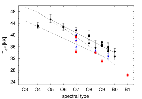
Figure 1 shows the distribution of the effective temperature as a function of O and early-B spectral sub-type for the investigated sample. The different luminosity classes are denoted using circles for the dwarfs and subgiants, triangles for the giants, and squares for the bright giants and supergiants. We now concentrate on dwarf stars only, which account for the vast majority in our sample. For these objects the figure shows a well defined relation, the mean of which is represented by the solid line. At the earliest spectral types (O4–O6) the relation seems to flatten out. However, the small number of objects analysed in this range make this part of the diagram uncertain. Moreover, two of the objects at spectral type O4 and O5 suffer from strong nebular contamination, complicating the determination of their effective temperature (see the appendix).

Shown with a dashed line in Fig. 1 is the $T_{\rm eff}$ “observational” calibration for Galactic O-type dwarf stars as derived by Martins et al. (2005a). A clear offset is apparent between this relation and the average calibration for the SMC O dwarfs. This offset is approximately 3.3 kK for the latest types up to approximately 4.4 kK for spectral type O5. These differences in $T_{\rm eff}$ correspond to a shift in spectral sub-type of about 2 for the late type objects and $\sim$1.5 sub-types for the earliest types. Mokiem et al. (2004), using cmfgen (Hillier & Miller, 1998) and covering the metallicity range from 2 times Solar to 1/10 Solar, find typical shifts of one sub-type, though we should add that this comparison is not as extensive as the one presented here.

Figure 1 also shows a clear separation between objects of different luminosity class. Compared to dwarfs, the giants, bright giants, and supergiants systematically have lower effective temperatures. The reason for this separation is twofold. First, the latter group of objects represent more evolved evolutionary phases. Their lower gravities result in an increased helium ionisation (e.g. Kudritzki et al., 1983), reducing the effective temperature associated with a given spectral type. Second, these objects are expected to have stronger stellar winds. This induces an increased line blanketing effect, further reducing the $T_{\rm eff}$ for a given spectral type.

Massey et al. (2005) also report a Sp.Type($T_{\rm eff}$) calibration for SMC stars. As can be seen in Fig. 1 their relation essentially agrees with ours at spectral types earlier than O8. However, at later types their results suggest a rather sharp turn towards the Martins et al. relation for Galactic stars which is not observed in our sample. The reason for this apparent discrepancy is that our calibration employs dwarfs, whilst Massey et al. had to rely upon giant stars at the latest O subtypes.

4.2 Ionising fluxes

The ionising fluxes of massive stars are important quantities that are used in the study of, for instance, H ii regions and starburst galaxies (e.g. Vacca, 1994). The parameter that is used to characterise the ionising output is the number of photons present in the Lyman continuum, $Q_{0}$. It is defined as

$$\mbox{$Q_{0}$}=4\pi^{2}R_{\star}^{2}\int_{0}^{\lambda_{0}}\frac{\pi\lambda F_{\lambda}}{hc}d\lambda\leavevmode\nobreak\ ,$$ (1)

where $F_{\lambda}$ and $\lambda_{0}$ are, respectively, the stellar flux in erg s^-1 cm^-2 Å^-1 and the limiting wavelength for photons able to ionise hydrogen, i.e. 912 Å.

Tables 3 and 4 list the number of ionising photons for the individual objects and the associated error estimates. These errors are dominated by the uncertainty in stellar radius and effective temperature. To calculate the error estimates we adopted an uncertainty of 0.03 dex in $R_{\star}$, which is dominated by the estimate for $\Delta$$M_{V}$. The error introduced by $\Delta$$T_{\rm eff}$ was estimated from Fig. 16 from Martins et al. (2005a), which shows the number of ionising Lyman continuum photons as a function of effective temperature for the line blanketed stellar atmosphere codes cmfgen, wm-basic and tlusty. The difference between the predictions of these three codes is relatively small and, consequently, we estimated the uncertainty introduced in $Q_{0}$ to be 0.09 dex/kK for $\mbox{$T_{\rm eff}$}>36$ kK and 0.18 dex/kK for $\mbox{$T_{\rm eff}$}<36$ kK.

Figure 2: Number of Lyman continuum ionising photons $Q_{0}$ as a function of spectral type. Different luminosity classes are shown using circles, triangles and squares for, respectively, IV-V, III and I-II class objects. Grey circles correspond to stars located on or left of the ZAMS. Indicated using a dashed line is the Galactic calibration for dwarfs from Martins et al. (2005a).

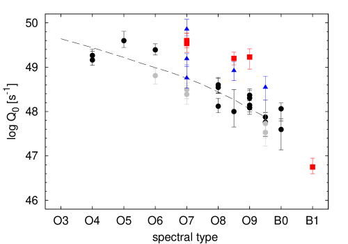
In Fig. 2 the distribution of $Q_{0}$ as a function of spectral type for our programme stars is presented. Different luminosity classes are indicated using circles, triangles and squares for respectively, IV-V, III and I-II class objects. On average the more evolved stars are found to produce more ionising photons for a given spectral type because of their larger radii, hence higher luminosities. Also shown in this figure as a dashed line is the “observational” $Q_{0}$ calibration for Galactic dwarfs from Martins et al. (2005a). In general we find that the ionising fluxes of the SMC dwarfs are in good agreement with this calibration (also see Mokiem et al., 2004). The most pronounced differences are for the O4 and O7 stars. With respect to the earliest spectral type this can be explained by nebular contamination hampering the $T_{\rm eff}$ determination (see previous section). The low ionising fluxes of the two O7 dwarfs, however, cannot be explained in this way, as they are found to follow the $T_{\rm eff}$ trend in Fig. 1. Instead, we believe that the discrepancy is related to their location in the HR-diagram, i.e. evolutionary phase. The two dwarfs are found to locate a position on or to the left of the ZAMS (see Sect. 7.2). As a result of this they are less luminous compared to objects of the same spectral type that are located to the right of the ZAMS. Consequently, the total number of ionising photons produced by these objects is smaller than the average associated with their spectral type.

Apart from the two dwarfs at spectral type O7 three additional stars were found to lie on or to the left of the ZAMS (see Sect. 7.2). As can be seen in Fig. 2, where we have highlighted all ZAMS stars using grey circles, these stars produce on average less ionising photons. Note that two dwarfs at O8 and O8.5 also seem to lie below the average. The O8.5 star has a below average $T_{\rm eff}$ for its spectral type (see Fig. 1). This explains its somewhat peculiar $Q_{0}$ behaviour. The O8 star below the average is NGC 346-050. It also has a temperature that is lower than the average for its spectral type, though not to the same extent as NGC 330-052. Interestingly, this object lies closest to the ZAMS (see Fig. 13) of all non-ZAMS stars, and seems to behave in terms of $Q_{0}$ in a similar manner as the ZAMS objects. We conclude that the ZAMS stars for given spectral type have $\sim$0.4 dex lower Lyman continuum photons.

4.3 Gravities

Figure 3: Distribution of the analysed SMC objects in the $\log\mbox{$T_{\rm eff}$}$ – $\log{{g}}_{\rm c}$ plane. Indicated with different symbols are luminosity class IV-V (circles), III (triangles) and I-II (squares). With exception of the subgiant NGC 346-026, the first group of objects are clearly separated from the more evolved objects. These more evolved objects seem to follow a trend of increasing surface gravity with increasing effective temperature.

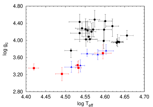
In Fig. 3 we present the distribution of SMC objects in the log $T_{\rm eff}$ – $\log{{g}}_{\rm c}$ plane. The surface gravity corrected for centrifugal acceleration ($\log{{g}}_{\rm c}$) was calculated according to the method discussed by Herrero et al. (1992) and Repolust et al. (2004). Different luminosity classes are indicated using circles, triangles, and squares for type IV-V, III, and I-II objects, respectively. With the exception of one object, the dwarf type objects are all above $\mbox{$\log{{g}}_{\rm c}$}\simeq 3.9$. The object with a lower gravity, NGC 346-026 is the only subgiant. The luminosity class I-III objects occupy a strip below the dwarfs, reflecting the evolutionary path of hot massive stars in this diagram. Note that no separation between luminosity class III and I-II objects is visible in this secular behaviour.

A comparison of the masses based on the spectroscopically determined surface gravities and those derived from predictions of massive star evolution is presented in Fig. 4. The different luminosity classes are distinguished using the same symbols as in Fig. 3. To determine the evolutionary masses evolutionary tracks from Charbonnel et al. (1993), for $Z=0.2\,\mbox{$Z_{\sun}$}$ were used. The errors in evolutionary mass reflect the mass interval allowed within the error box spanned by the stellar luminosity and effective temperature. As the tracks of Charbonnel et al. do not account for the effects of rotation, this source of error is not included. Predictions accounting for $v_{\rm rot}$ show complicated tracks including loops during the secular redward evolution. Therefore, one can no longer assign an unambiguous $M(L,\mbox{$T_{\rm eff}$})$. Still, assessing the impact of rotation using the Maeder & Meynet (2001) and Meynet & Maeder (2005) computations that adopt an initial rotational velocity $\mbox{$v_{\rm r}$}=300\,\mbox{km\,s${}^{-1}$}$ shows that the error in the evolutionary mass will not increase by more than $\sim$13 percent. The errors in the spectroscopic mass are much larger than those in $M_{\rm ev}$, and primarily reflect the error in gravity.

Figure 4: Comparison of spectroscopically determined masses with masses derived from the evolutionary tracks of Charbonnel et al. (1993) for $Z=0.2\,\mbox{$Z_{\sun}$}$. Denoted by circles, triangles and squares are, respectively, luminosity classes IV-V, III and I-II. The dashed line corresponds to the one-to-one relation between the two mass scales. With exception of the two most massive objects, no systematic discrepancy between the spectroscopic and evolutionary masses is observed.

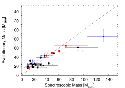
Inspection of Fig. 4 reveals no convincing systematic discrepancy between the spectroscopic and evolutionary mass, even though some objects do not agree within their standard deviation with the one-to-one relation. At the low mass end there appears to be some tendency for the spectroscopic masses to be less than those from evolutionary tracks. This behaviour is similar to the “mass discrepancy problem” reported and discussed by e.g. Herrero et al. (2002) and Repolust et al. (2004). Note that most of this classical problem has been resolved, i.e. it has been attributed to limitations of the stellar atmosphere models (Herrero, 1993) and biases in the fitting process (see Paper I). With respect to the stars at the low mass end, we note that star NGC 346-107 occupies a location in the HR-diagram left of the ZAMS (see Fig. 6). As the evolutionary status of this object is formally not defined, the mass that is given is based on an extrapolation of the tracks. This could lead to an erroneous value of $M_{\rm ev}$. Interestingly, for the other stars at the low mass end the helium abundances listed in Tab. 3 seem to correlate with the mass discrepancy. We will investigate this in detail in the next section. Also note that Massey et al. (2005) identify a mass discrepancy in a sample of Magellanic Cloud stars for objects with $\mbox{$T_{\rm eff}$}\gtrsim 45$ kK, which they attribute to a possible underestimation of $\log{{g}}$ by the model atmospheres. Unfortunately, our sample does not contain enough early-type O stars to corroborate the findings of these authors.

For the two brightest objects, AzV 14 and AzV 26, the spectroscopic masses are much larger than the implied evolutionary masses. The profile fits, in particular those of the gravity sensitive hydrogen Balmer lines, (see the appendix) are good. So, it is not likely that the reason for the discrepancy is an overestimation of the spectroscopically determined gravity. One could speculate about a possible binary nature of both stars, as the spectroscopic mass is more sensitive to changes in luminosity. An indication of binarity may be the conspicuously high luminosities. However, using spectroscopic and spectral morphological arguments, Massey et al. (2004) tentatively rule out a composite explanation for both objects. In contrast to this we note that the luminosity and derived mass-loss rate for these two stars (see Sect. 4.6) imply a position in the modified wind momentum vs. luminosity diagram which is well below what is expected from theory, i.e. the mass loss for these two stars would be in better agreement with predictions if their luminosity would be lower.

4.4 Helium abundances

Figure 5: Helium abundances as a function of surface gravity. Luminosity classes IV-V, III and I-II are denoted using circles, triangles and squares, respectively. Open symbols correspond to fast rotators ($\mbox{$v_{\rm r}\sin i$}>250\,\mbox{km\,s${}^{-1}$}$). The average helium abundance of the investigated sample is 0.13. Shown with a dashed line is a measure for the initial $Y_{\rm He}$, which is taken to be the average of the helium abundances of the dwarfs with a $Y_{\rm He}$ smaller than the sample average. Compared to this “initial” abundance of 0.09 an increase in $Y_{\rm He}$ is visible for decreasing surface gravity.

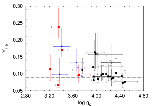
The automated method also treats the helium abundance as a continuous free parameter. Usually, spectroscopic analyses assume an initial Solar value for $Y_{\rm He}$, which is only modified when no satisfying fit can be obtained (e.g. Herrero et al., 2002; Repolust et al., 2004; Massey et al., 2004). Because of the automated treatment and the extent of our sample we can, for the first time rigorously, investigate possible correlations between the surface helium abundance and other fundamental parameters.

In Fig. 5 we show $Y_{\rm He}$ as a function of surface gravity $\log{{g}}_{\rm c}$. The horizontal dashed line represents the initial helium abundance of the SMC stars investigated. It corresponds to the average of the helium abundances of the dwarf objects with $Y_{\rm He}$ smaller than the total sample average. Using this “initial” abundance of $0.09^{+0.009}_{-0.004}$ as a reference, the overall trend is that the average $Y_{\rm He}$ increases for decreasing surface gravity. This is consistent with the standard picture that more evolved objects may have their atmospheres enriched with primary helium. Interestingly, however, one may immediately spot two deviating objects from the overall trend. First, the supergiant NGC 346-012 has a helium abundance lower than the “initial” value. This object has $\mbox{$\log{{g}}_{\rm c}$}=3.35$ and $\mbox{$Y_{\rm He}$}=0.07$. The reason for the low surface helium abundance is unclear and we will exclude this star from the remainder of this discussion.

Second, some of the unevolved objects have enhanced helium abundances. It can therefore be suspected that more parameters are involved in controlling the enrichment displayed in Fig. 5. One such parameter could be stellar rotation. Meynet & Maeder (2000), for instance, predicted that extensive mixing in fast rotators could result in significant surface helium enhancement relatively early in the evolution. To probe this possibility we have highlighted the fast rotators, defined as having $\mbox{$v_{\rm r}\sin i$}>250\,\mbox{km\,s${}^{-1}$}$, in Fig. 5 using open symbols. In case of all four fast rotators we see that their helium abundances are enhanced with respect to the “initial” value, suggesting that the helium enhancement may be (partly) related to fast rotation. This may imply that two other dwarf objects with a clear helium enhancement ($\mbox{$Y_{\rm He}$}\approx 0.16$) but with low projected rotational velocity are in fact fast rotators seen pole on.

Figure 6: HR-diagram of the analysed SMC sample. Different luminosity classes are distinguished using identical symbols as used in Fig. 5. Open symbols correspond to objects with a helium abundance of at least 0.12. Over-plotted in grey are the evolutionary tracks of Maeder & Meynet (2001) and Meynet & Maeder (2005) with $Z=0.2\,\mbox{$Z_{\sun}$}$ and $\mbox{$v_{\rm r}$}=300\,\mbox{km\,s${}^{-1}$}$. The ZAMS corresponding to these tracks is shown as a black solid line. The grey area in the top part of the diagram corresponds to the region in which the evolutionary models exhibit an enhancement of the surface helium abundance by ten percent or more.

How well do our spectroscopically derived helium abundances compare to those predicted by evolutionary models? This is a fundamental but complicated question. Important to realise is that one of the effects of rotation is that it introduces a wide bifurcation in the evolutionary tracks. Stars rotating above a threshold $v_{\rm r}$ of about 30–50 percent of break-up (depending on initial mass; Yoon & Langer 2005) follow tracks which are essentially those of chemically homogeneous evolution. Such tracks do not evolve towards the red in the HRD, but evolve bluewards (from the zero age main sequence) and upwards until the star enters the Wolf-Rayet phase (Maeder, 1987). Stars rotating below this critical value evolve along tracks which are about similar to non-rotating ones, though at an earlier age the surface abundances of helium (and carbon, nitrogen and oxygen) will be affected by rotation induced mixing.

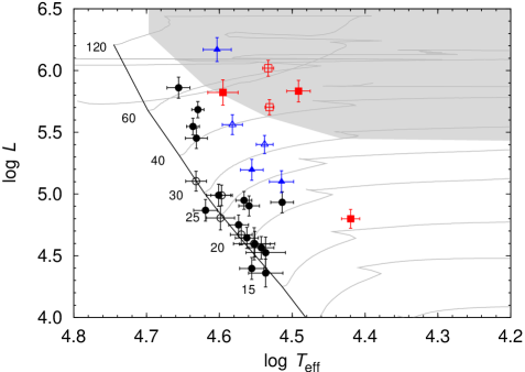
Let us first compare our results with tracks for rotational velocities below this critical value. In the HR-diagram shown in Fig. 6 the grey lines correspond to evolutionary predictions by Maeder & Meynet (2001) and Meynet & Maeder (2005), which were calculated for $Z=0.2\,\mbox{$Z_{\sun}$}$ and $\mbox{$v_{\rm rot}$}=300\,\mbox{km\,s${}^{-1}$}$. Objects for which a spectroscopic helium abundance of at least $\mbox{$Y_{\rm He}$}=0.12$ was found are denoted using open symbols. Note the location of four helium rich dwarf stars close to or even on the ZAMS. These will be discussed in more detail in Sect. 7. The grey area in the figure corresponds to the region in which the evolutionary models predict a surface helium enhancement of at least ten percent.

The regime in which the evolved stars showing significant helium surface enrichment reside roughly coincides with the location of the grey area. Not all evolved objects show evidence of $Y_{\rm He}$ enrichment. Many exhibit an abundance about equal to the initial value. None of these stars are fast rotators (they all have $\mbox{$v_{\rm r}\sin i$}\lesssim 140\mbox{km\,s${}^{-1}$}$). This can easily be explained using tracks for non-rotating stars (Meynet & Maeder, 2000). The fair consistency between observed and predicted helium abundance in evolved objects is reassuring, however, a more detailed comparison requires the availability of tracks for several more values of $v_{\rm rot}$.

Figure 7: The mass discrepancy (see also Fig. 4) as a function of surface helium abundance. To compute the discrepancy non-rotating tracks of Charbonnel et al. (1993) are used. Circles, triangles, and squares denote dwarfs, giants, and supergiants, respectively. The open circles indicate stars on or left of the ZAMS. The bulk of the stars has the initial helium abundance $\mbox{$Y_{\rm He}$}=0.09$ where the discrepancy seems random and of the order of the error. For helium enriched stars the discrepancy always favours a higher $M_{\rm ev}$, qualitatively consistent with models accounting for mixing increasing the $M/L$-ratio and bringing helium to the surface. A quantitative prediction (short dashed lines) based on ZAMS stars of 20 (upper curve) and 30 $M_{\sun}$ (lower curve) varying helium abundance shows, however, a more modest effect than implied by our findings.

We mentioned above that for modest rotation the tracks do not differ greatly from non-rotating ones. This is not completely correct as rotation tends to make the star somewhat more luminous. Langer (1992) proposed that this might explain the mass discrepancy problem identified by Herrero et al. (1992). Although recent analyses no longer suggest a convincing systematic discrepancy (see e.g. Sect. 4.3), it is still interesting to look at this idea in some more detail. Langer connects the apparent mass problem to the helium abundance by showing that the $M/L$-ratio is a monotonically decreasing function for increasing helium enrichment. Consequently, if mixing brings primary helium to the surface one expects the star to be overluminous, leading to an overestimate of the evolutionary mass if non-rotating tracks are adopted. If indeed this is the case, then the scatter around the one-to-one relation in Fig. 4 might reveal a trend when plotted against $Y_{\rm He}$.

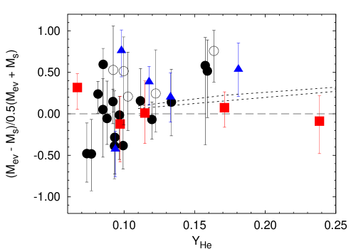
The result of this exercise is shown in Fig. 7. On the vertical axis a measure of the mass discrepancy is given. Note that the mass difference is plotted relative to the mean of the evolutionary and spectroscopic mass to ensure that positive and negative discrepancies are shown on the same linear scale. For the evolutionary masses, tracks that do not account for rotation are used. The circles, triangles, and squares denote dwarfs, giants, and supergiants, respectively. The open circles indicate stars on or left of the ZAMS. At the “initial” helium abundance of $\mbox{$Y_{\rm He}$}=0.09\pm 0.01$ – where most of the stars reside and dwarfs dominate – the scatter around the $\mbox{$M_{\rm ev}$}=\mbox{$M_{\rm s}$}$ relation appears random. This essentially reflects that there is no systematic mass discrepancy. At $0.13\lesssim\mbox{$Y_{\rm He}$}\lesssim 0.19$ the scatter is not random, as all objects show a positive mass discrepancy. In principle this is qualitatively consistent with the above described idea. However, is it also quantitatively consistent? To assess this we have computed the mass discrepancy for ZAMS stars with a variable helium abundance. This should reflect the maximum effect of rotation, i.e. such effective mixing that it leads to chemically homogeneous evolution. The results for stellar masses of 20 and 30 $M_{\sun}$ – typical for the bulk of our sample – are shown (short dashed lines). These predictions clearly show a more modest mass discrepancy, though the error bars on the mass discrepancy for the programme stars do reach these predictions. We conclude that stars with an enriched helium surface abundance tend to show a systematic mass discrepancy that is qualitatively consistent with predictions of chemically homogeneous evolution. We finally note that the supergiants in our sample, which can be explained using evolutionary models including rotation, show the best agreement between $M_{\rm ev}$ and $M_{\rm s}$ (see also Fig. 4).

4.5 Microturbulence

Similar to the helium abundance the fact that the microturbulent velocity is treated as a free parameter allows us for the first time to investigate possible correlations for this parameter. However, in contrast to the former parameter, this investigation did not yield any clear relation between $v_{\rm turb}$ and any other parameter. For each parameter given in Tab. 3 a comparison with the microturbulent velocity basically results in a scatter diagram. This null result is similar to the findings in Paper I and reflects the uncertainty with which $v_{\rm turb}$ can be determined from the hydrogen and helium spectrum. Apparently the line profiles are not very sensitive to this parameter.

Figure 8: Modified wind momentum ($D_{\rm mom}$) in units of ${\rm g\,cm\,s^{-2}}\,\mbox{$R_{\sun}$}$ as a function of luminosity for the analysed SMC sample. Luminosity classes are distinguished using identical symbols as in Fig. 5. Indicated using grey inverted triangles are upper limits. At $\log\mbox{$L_{\star}$}/\mbox{$L_{\sun}$}\approx 5.0$ the open symbol indicates the location NGC 346-033 would have if its true $v_{\infty}$ would be lower by a factor two compared to the adopted value. Using open squares modified wind momenta corrected for clumping are shown for the two supergiants with H$\alpha$ emission profiles. The upper and lower dashed lines correspond to the theoretical wind-momentum luminosity relations (WLR) as derived by Vink et al. (2000, 2001) for, respectively, Galactic and SMC metallicity. Shown with a dotted line is the empirical WLR constructed for objects with $\log\mbox{$L_{\star}$}/\mbox{$L_{\sun}$}\gtrsim 5.4$.

We should also consider the fact that the error estimates determined for $v_{\rm turb}$, as given in Tab. 4 are on average considerably large. As a result of this, one could argue that for many objects it simply was not possible to accurately determine $v_{\rm turb}$. Consequently, it is not possible to find any correlation when the total sample is considered. To avoid this potential problem we also investigated possible correlations using a subset of 14 objects for which the microturbulent velocity was determined relatively well. The selection criterion for this subset was that the $v_{\rm turb}$ error bars should be well confined within the search domain, spanning the range of 0 up to 20 km s^-1. The comparison within the subset again did not result in a correlation for $v_{\rm turb}$ with any of the other parameters.

4.6 Wind parameters

Our sample is dominated by late O-type dwarf stars, which are expected to have relatively weak winds. These are so weak that they challenge the sensitivity of H$\alpha$ as a mass-loss diagnostic. With nebular contamination as an additional complicating factor, we could not derive reliable $\dot{M}$ for all objects. For nineteen stars (see Tab. 3) we can only derive upper limits, i.e. the downward error bars on our fit extend to the lower limit of the $\dot{M}$ regime in which the automated method was allowed to search for a solution. It happens to be so that these can be identified by an error bar $-\log\Delta\mbox{$\dot{M}$}\gtrsim 1.0$ dex (see Tab. 3). For many stars we could also not determine the acceleration behaviour of the wind, expressed by the exponent $\beta$ of the velocity law. For these objects we adopted $\beta=0.8$ consistent with theoretical expectations (Pauldrach et al., 1986).

Despite the large number of upper limits, it is still possible to quantitatively investigate the SMC stellar winds. We do this by studying the distribution of the analysed objects in the so-called modified stellar wind momentum vs. luminosity diagram. The modified wind-momentum, which is defined as $\mbox{$D_{\rm mom}$}\equiv\mbox{$\dot{M}$}\mbox{$v_{\infty}$}R^{1/2}_{\star}$, is predicted to behave as a power-law as a function of stellar luminosity (Kudritzki et al., 1995; Puls et al., 1996)

$$\log\mbox{$D_{\rm mom}$}=x\log\left(\mbox{$L_{\star}$}/\mbox{$L_{\sun}$}\right)+\log D_{\circ}\leavevmode\nobreak\ .$$ (2)

In the above equation $x$ corresponds to the inverse of the slope of the line-strength distribution function corrected for ionisation effects (Puls et al., 2000) and $D_{\circ}$ is a measure for the effective number of lines contributing to the acceleration of the wind.

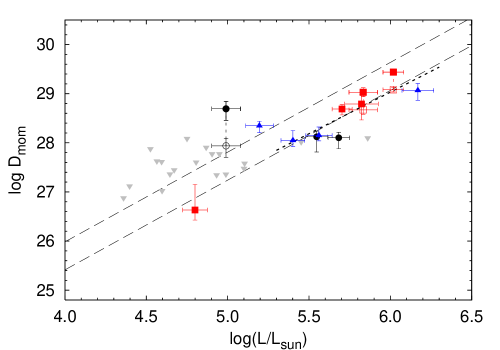
In Fig. 8 we present the distribution of the modified wind momenta of our sample. The upper dashed curve is the theoretical prediction for a Galactic metal content; the lower dashed curve is that for an SMC metallicity (Vink et al. 2001; see also below), which is predicted to be shifted downward by 0.57 dex with respect to the Galactic relation. Before confronting theory with observations, we first discuss a few individual objects. The $D_{\rm mom}$ upper limit at $\log\mbox{$L_{\star}$}/\mbox{$L_{\sun}$}\approx 5.9$ corresponds to the object AzV 14. As was argued in Sect. 4.3, this object might be over-luminous because of a binary nature.

The O8 V star NGC 346-033 (at $\log\mbox{$L_{\star}$}/\mbox{$L_{\sun}$}\approx 5.0$) is positioned far above the SMC prediction. We suspect this is connected to the anomalously high terminal velocity of 4100 km s^-1, which results from a scaling with $v_{\rm esc}$ as no direct UV measurement is available. If this $v_{\infty}$ would be overestimated by a factor of two (for an O8 V star one would expect $\mbox{$v_{\infty}$}\sim 1900\,\mbox{km\,s${}^{-1}$}$, cf. Kudritzki & Puls 2000) the $D_{\rm mom}$ would be reduced by approximately a factor of six. This is so because $D_{\rm mom}$ scales directly with $v_{\infty}$ and indirectly with $\mbox{$v_{\infty}$}^{3/2}$ through the invariant wind-strength parameter ($Q\propto\mbox{$\dot{M}$}/\mbox{$v_{\infty}$}^{3/2}$, e.g. see Puls et al. 2005). The open circle shows the effect of such a decrease in terminal velocity. We decided to exclude this object from the remainder of this discussion.

The two O-type supergiants in our sample, AzV 372 and NGC 346-001, are the only two exhibiting an H$\alpha$ emission profile. Markova et al. (2004) and Repolust et al. (2004) have argued that for such stars the mass loss may be overestimated relative to dwarf stars due to wind clumping effects. For dwarf stars the H$\alpha$ absorption line is formed relatively close to the stellar surface, where clumping may be negligible. The H$\alpha$ emission line is typical for supergiants and in contrast reflects that the line is formed over a larger volume, where – they propose – clumping has set in. Indeed, for NGC 346-001 Crowther et al. (2002) present evidence for wind clumping based on the analysis of the UV phosphorus lines. Repolust et al. (2004) derive a correction for this clumping by multiplying the mass loss by a factor 0.44, which we have applied for the two objects. The corrected modified wind-momenta are shown in Fig. 8 using open squares.

For SMC objects, Fig. 8 represents the best populated modified wind-momentum diagram presented so far (12 mass loss determinations and 19 upper limits). In particular at $\log\mbox{$L_{\star}$}/\mbox{$L_{\sun}$}\gtrsim 5.4$ we find excellent agreement with the Vink et al. predictions, establishing that at these luminosities the winds of SMC stars are weaker, in accord to theoretical expectations. At $\log\mbox{$L_{\star}$}/\mbox{$L_{\sun}$}\lesssim 5.2$ the situation is less clear as for many stars we could only set upper limits and for those for which $\dot{M}$ could be derived the error bars are large. For the weak wind regime we therefore cannot draw firm conclusions.

We have constructed an empirical WLR by fitting a linear function to the objects in Fig. 8 with $\log\mbox{$L_{\star}$}/\mbox{$L_{\sun}$}\gtrsim 5.4$, while accounting for the symmetric errors in luminosity and the asymmetric errors in $D_{\rm mom}$. Using the clumping corrected $D_{\rm mom}$ values for AzV  372 and NGC 346-001 this results in the following relation

$$\log\mbox{$D_{\rm mom}$}=(1.69\pm 0.34)\log\left(\mbox{$L_{\star}$}/\mbox{$L_{\sun}$}\right)+(18.87\pm 2.00)\leavevmode\nobreak\ ,$$ (3)

which is shown in Fig. 8 as a dotted line. Within the error bars the fit parameters agree with the theoretical calculations of Vink et al. (2001), who predict $x=1.83$ and $\log D_{\circ}=18.11$ for SMC metallicity. To illustrate the agreement we compare the predicted and fitted wind momenta at the boundaries of the fitting range. For $\log\mbox{$L_{\star}$}/\mbox{$L_{\sun}$}=5.4$ and $\log\mbox{$L_{\star}$}/\mbox{$L_{\sun}$}=6.2$ the differences are $-0.02$ dex and $0.08$ dex, respectively. Given the fact that the typical uncertainty in $D_{\rm mom}$ is of the order of 0.2 dex, we find the agreement excellent. We note that the weak wind regime is discussed in more detail in Sect. 6.

4.7 Projected rotational velocities

Figure 9: Comparison of $v_{\rm r}\sin i$ distributions. Left panel: cumulative distribution functions (cdf) of $v_{\rm r}\sin i$ for unevolved objects, i.e. luminosity class IV and V, and evolved objects, i.e. luminosity class I, II, III, in the SMC. The group of unevolved SMC objects are found to contain relatively both more fast rotators ($\mbox{$v_{\rm r}\sin i$}\gtrsim 100\,\mbox{km\,s${}^{-1}$}$) as well as more slow rotators ($\mbox{$v_{\rm r}\sin i$}\lesssim 50\,\mbox{km\,s${}^{-1}$}$) with respect to the group of evolved objects. Right panel: cdf of unevolved SMC objects and unevolved Galactic objects (Penny, 1996). Compared to the Galactic sample the SMC sample contains a larger fraction of intermediately fast rotating stars ($120\gtrsim\mbox{$v_{\rm r}\sin i$}\lesssim 190\,\mbox{km\,s${}^{-1}$}$).

The projected rotational velocities as determined with the automated fitting method are listed in Tab. 3. The associated uncertainties range from approximately 10 km s^-1 for the slow rotators up to about 40 km s^-1 for the fast rotators, indicating that we were able to accurately determine $v_{\rm r}\sin i$ with our self consistent method. Note that the low $v_{\rm r}\sin i$ of NGC 346-031 and NGC 346-051 are close to the effective resolution of the FLAMES observation ($\sim$15 km s^-1), and should be interpreted as upper limits.

If a star rotates at more than approximately 80% of critical rotation the assumption of spherical symmetry may break down (e.g. Maeder & Meynet, 2000). Checking the ratio $\mbox{$v_{\rm r}\sin i$}/v_{\rm crit}$ for all our target stars, we find a maximum of about $\sim$0.65. We therefore do not expect any significant deviations from sphericity, nor uncertainties in the derived parameters due to rotational effects.

4.7.1 Rotation vs. macroturbulence

In our calculations we consider the possibility of small scale velocity fields. These thermal and microturbulent motions have a coherence length that is small compared to the line forming region. We do not include the possibility of motions that have a coherence length that is comparable to or is larger than the line forming zone. Such motions are denoted with the term macroturbulence ($v_{\rm mac}$). If a large macroturbulent velocity field is present, it may be expected that the projected rotational velocity that we determine from the hydrogen and helium profiles is overestimated.

To assess the importance of macroturbulence we have also determined $v_{\rm r}\sin i$ by means of a Fourier technique (Simón-Díaz et al., 2006) using weak metal lines as an independent diagnostics. The Fourier technique allows to discriminate between macroturbulence and rotation, as it is sensitive to differences in the rotational and macroturbulent profiles (see e.g. Gray, 1978). For details on this method we refer to Simón-Díaz et al. In all but one case we get $v_{\rm r}\sin i$ values that are consistent to within the error estimates. As in first order the $v_{\rm r}\sin i$ and $v_{\rm mac}$ broadening should be added quadratically, this does not necessarily imply that macroturbulent motions are absent. For $v_{\rm r}\sin i$ of order 100 to 150 km s^-1, macroturbulent fields with characteristic velocities of up to several tens of kilometres per second, i.e. comparable to the small scale velocity component, remain a possibility. Obviously, rapid rotators may show larger $v_{\rm mac}$ components.

For the O8.5 bright giant AzV 469 the Fourier method recovers a $v_{\rm r}\sin i$ that is about 30 percent lower than the 81 km s^-1 derived from the hydrogen and helium profiles. This could indicate the presence of a macroturbulent velocity field with $\mbox{$v_{\rm mac}$}\sim 50\,\mbox{km\,s${}^{-1}$}$. Significant macroturbulent fields have been reported for B supergiants (e.g. Ryans et al., 2002), but not for early O-type stars. The fact that this star is of relatively late O sub-type seems consistent with these findings. Consequently, in the $v_{\rm r}\sin i$ distribution analysis presented below we adopt the projected rotational velocity for AzV 469 as determined using the Fourier method.

4.7.2 Observed $v_{\rm r}\sin i$ distributions

For a meaningful comparison of the distribution of the projected rotational velocities of the SMC objects with other observations and with theory we use cumulative distribution functions (cdfs). The cdf describes the distribution of $v_{\rm r}\sin i$ by simply giving for every observed $v_{\rm r}\sin i$ the fraction of objects with lower or equal velocities. In Fig. 9 the cdfs of the SMC sample are presented and compared to cdfs of Galactic O-type stars.

The left panel in Fig. 9 compares the cdfs of unevolved objects, i.e. luminosity class IV and V, and evolved objects, i.e. luminosity class I, II and III, in the SMC. This comparison shows that compared to the evolved objects the group of unevolved objects contain relatively more fast rotators. For instance, approximately ten percent of the evolved objects have a $v_{\rm r}\sin i$ in excess of 150 km s^-1, whereas approximately 40 percent of the unevolved objects exhibit velocities larger than this $v_{\rm r}\sin i$. Note that about 20 percent of the group of unevolved objects is rotating slowly ($\mbox{$v_{\rm r}\sin i$}\lesssim 50\,\mbox{km\,s${}^{-1}$}$), while this is only 10 percent for the evolved stars.

Using the Kolmogorov-Smirnov (K-S) test we have determined that the probability that the two samples are drawn from the same underlying distribution is 23 percent. Therefore, the differences between the cdfs of the unevolved and evolved SMC stars may be significant and possibly not due to statistical fluctuations. The trend that is found here is also seen in Galactic O-type stars. Using a similar approach, Howarth et al. (1997) and Penny et al. (2004) also find relatively more slow and fast rotators among the unevolved stars (also see Conti & Ebbets, 1977). Howarth et al. ascribe the reduced number of fast rotators to spin down as a result of an increased radius for the evolved stars, as well as to loss of angular momentum through the stellar wind. This explanation may also apply to the SMC case. They further suggest that the apparent lack of slow rotating evolved stars is a spurious result, caused by erroneously assigning turbulent broadening – which is more pronounced for evolved stars (Ryans et al., 2002) – to rotational broadening. As a result, the derived $v_{\rm r}\sin i$ are overestimates, therefore some $v_{\rm r}\sin i$ larger than 50 km s^-1 (causing the steep gradient of the dashed curve in the left panel at about $70-80\,\mbox{km\,s${}^{-1}$}$) in reality reflect projected rotational velocities below 50 km s^-1. For this to be the correct explanation, the required turbulent velocities should be large (order $40-70\,\mbox{km\,s${}^{-1}$}$). Whether such an explanation is valid for our sample is doubtful, as we have found no indication for the existence of significant macroturbulent velocities in the objects with $\mbox{$v_{\rm r}\sin i$}\lesssim 100\,\mbox{km\,s${}^{-1}$}$.

In the right panel of Fig. 9 the 21 unevolved SMC objects are compared to 66 unevolved Galactic stars as measured by Penny (1996). Again using the Kolmogorov-Smirnov test we determined that the probability that the two samples have the same underlying distribution is 13%. Therefore, we tentatively assume that the SMC distribution of unevolved stars is significantly different from the Galactic distribution. However, this should be verified using a larger sample of SMC objects.

Figure 10: Left panel: cdfs of observed (solid line) and theoretical initial $v_{\rm r}\sin i$ distributions. Dotted and dashed lines, respectively, correspond to a constant $v_{\rm r}$ distribution, i.e. block function, and a single value $v_{\rm r}$ distribution. Right panel: filled areas indicate the one $\sigma$ probability distribution for theoretical $v_{\rm r}\sin i$ cdfs for the limited number of 21 objects calculated from a constant $v_{\rm r}$ distribution with $\mbox{$v_{\rm min}$}=0\,\mbox{km\,s${}^{-1}$}$ and $v_{\rm max}$ of 200, 352 or 600 km s^-1. Shown with a dotted, dashed and dashed-dotted curve are, respectively, the best fitting block function, Gaussian and Maxwellian distribution cdf. See text and Fig. 11 for further comments and explanation.

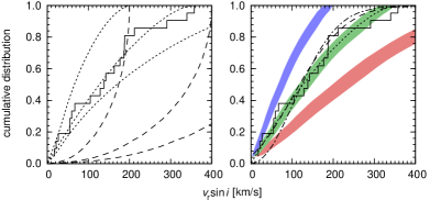
A marked difference between the two curves is the behaviour between the intersection points at $\sim$90 and $\sim$190 km s^-1. The fact that these curves intersect at these two points reflects that for both the SMC and Galaxy the same fraction of stars show projected rotational velocities in this range. However, the fact that in between 90 and 190 km s^-1 the Galactic curve lies above the SMC one implies that the Galactic stars show preferably lower $v_{\rm r}\sin i$ (i.e. closer to 90 km s^-1) than in the SMC. This behaviour is consistent with the SMC stars suffering less from spin down due to mass loss, as the SMC stars are expected to have weaker winds. The behaviour outside of the above velocity range cannot be understood within the context of spin down through winds. At $\mbox{$v_{\rm r}\sin i$}\lesssim 90\,\mbox{km\,s${}^{-1}$}$ the SMC shows preferably larger projected rotational velocities; at $\mbox{$v_{\rm r}\sin i$}\gtrsim 190\,\mbox{km\,s${}^{-1}$}$ both galaxies show the same distribution. If the Galactic objects indeed suffer from a stronger spin down, the latter behaviour could in principle imply that star formation in a relatively metal rich environment results in larger initial rotational velocities. However, note that the SMC cdf for $\mbox{$v_{\rm r}\sin i$}>200\,\mbox{km\,s${}^{-1}$}$ only contains four objects, which makes this last statement very uncertain.

The scenario in which SMC stars suffer less from spin down is consistent with the recent analysis performed by Dufton et al. (2006) for the young Galactic cluster NGC 6611. They find that the $v_{\rm r}$ distribution of the O-type stars can be characterised by a Gaussian with a mean of $\sim$125 km s^-1. In the next section we will show that the underlying $v_{\rm r}$ distribution of our SMC stars can be fitted by a Gaussian with a mean of $\sim$160 km s^-1. Consequently, as the age of NGC 6611 ($\sim$2 Myr) is comparable to the age of NGC 346, it appears that the weaker winds of the SMC objects result in less spin down in the first few million years of evolution.

It would be interesting to compare the evolved SMC and Galactic cdfs as the effect metallicity has on stellar rotation would likely be much more pronounced. However, for our sample this is not possible. The reason is that in the Galactic sample of Penny (1996) the ratio of luminosity class I-II to class III objects is a factor two larger compared to our SMC sample. Consequently, when making this comparison we could be confusing evolutionary effects with metallicity effects.

5 Parent rotational velocity distribution

The effect of rotation on the evolution of massive stars has been studied by e.g. Heger & Langer (2000), Meynet & Maeder (2000) and Maeder & Meynet (2001). This has shown that rotation may cause extensive mixing, changing the size of the reservoir of nuclear fuel available for evolution, and thus the lifetimes and tracks (e.g. Langer & Maeder, 1995). The effect of metal content on the time evolution of the surface equatorial velocity as a function of metal content is nicely illustrated in Figure 10 of Meynet & Maeder (2000) and Figure 3 in Maeder & Meynet (2001). The first figure shows this evolution for different stellar masses in a Galactic environment, using an initial surface equatorial velocity of 300 km s^-1. The second figure is identical, but now for a SMC environment. Ignoring the first $\sim$$10^{5}$ yrs – which show a rapid decrease of $v_{\rm eq}$ from $\sim$300 to $\sim$250 km s^-1, reflecting the initial convergence of the rotation law – the main sequence phase shows a monotonic decline of the equatorial rotational velocity as a result of an increasing radius and mass loss. Using the 20 $M_{\sun}$ track as an example, $v_{\rm eq}$ has reduced from $\sim$250 to $\sim$120 km s^-1 at the end of the main sequence phase in the case of Galactic stars, but to only 200 km s^-1 for SMC stars. The main fraction of the SMC decline occurs near the end of the main sequence phase; halfway the main sequence, $\mbox{$v_{\rm eq}$}\sim 230\,\mbox{km\,s${}^{-1}$}$. The reason for the modest decline of the SMC star is the fact that its stellar wind is weaker than that of its Galactic counterparts. Note that for an initially 60 $M_{\sun}$ SMC star, which has a stronger wind than the 20 $M_{\sun}$ star, wind effects do play an important role. Most stars in our unevolved SMC sample, however, have masses of about $\sim$15–30 $M_{\sun}$, therefore are representative for the discussed case. Given that the age of the NGC 346 cluster is about 1–3 Myr (see Sect. 7), we may conclude that – based on the evolution models – the observed cdf of the unevolved SMC objects should lie close to the initial cdf. This allows to address the interesting question: what is the initial $v_{\rm r}\sin i$ distribution?

5.1 initial $v_{\rm r}$ distributions

We compare the cdf of the unevolved SMC objects with the theoretical predictions. To calculate these theoretical cdfs we constructed simple models of the underlying unprojected rotational velocity distribution. For each distribution function we synthesised a theoretical distribution using a large number of objects ($N=10^{4}$), while assuming randomly oriented rotation axes. The four adopted models are:

1. a delta function, i.e. one single possible value of $v_{\rm r}$ for all objects;

2. a block function, i.e. a constant distribution of objects between a minimum velocity $v_{\rm min}$ and a maximum velocity $v_{\rm max}$;

3. a Gaussian distribution, with a mean velocity $v^{\rm G}_{r}$ and a standard deviation $\sigma$;

4. a Maxwellian distribution, specified by the most likely velocity $v^{\rm M}_{r}$;

The normalised distributions of (best fits of the) latter three models are shown in the right panel of Fig. 10. Results for the delta and block function are presented in the left panel of Fig. 10. The top, middle, and bottom dashed curve correspond to a population with a single rotational velocity $v_{\rm r}$ = 200, 400, and 600 km s^-1, respectively. From a comparison with the SMC distribution, we find that models assuming a single valued underlying $v_{\rm r}$ distribution fail to reproduce the observed cdf. Consequently, it is very unlikely that the velocity distribution of massive stars in this cluster can be characterised by a single rotational velocity. This immediately implies that the initial $v_{\rm r}$ distribution of this young cluster is not such that, for instance, massive stars are all born rotating at critical velocity. Such a supposition would not be completely unreasonable as the initial angular momentum of Jeans-unstable molecular cloud fragments is so large that – if one assumes it to remain conserved during collapse leading to the formation of a single object – all stars would have to rotate super-critical. Such rapid rotation must lead to the ejection of material and angular momentum, at least until the star is rotating at break-up velocity. As pointed out, the observed $v_{\rm r}\sin i$ distribution does not support such a scenario (also see Herrero & Najarro, 2005).

The dotted curves in the left panel of Fig. 10 correspond to the theoretical cdfs calculated for the second model, i.e. the block function. The best fit to the observations requires $v_{\rm min}$ = 0 km s^-1 and $v_{\rm max}$ = 352 km s^-1. For comparison, we also plot the result for $v_{\rm max}$ = 200 (top curve) and 600 km s^-1(bottom curve). We see that the overall shape of this model is in better agreement with the observed cdf and that the best fit model gives a good fit to the SMC stars.

Given the fact that the SMC cdf is constructed from a limited number of objects, we should also try to account for the effect that a small sample size has on the distribution in the theoretical cdfs. To do this we use the following approach. Instead of using a large number of simulated objects to calculate the theoretical cdf, we use a number equal to the amount of observed objects. Using different sets of random inclination angles we then calculate an ensemble of theoretical cdfs. The resulting distribution of these cdfs in the ensemble then describes the effect of statistical fluctuations due to a limited sample size. In the right panel of Fig. 10 the results of this approach are shown for the theoretical cdfs with underlying constant $v_{\rm r}$ distributions. The filled areas in this panel correspond to the ranges in the diagram containing one $\sigma$, i.e. 68 percent, of the theoretical cdfs. In other words the surfaces correspond to the area in which one can expect a theoretical cdf to be located within a one $\sigma$ probability. The top, middle and bottom areas, again, correspond to distributions with $v_{\rm max}$ equal to, respectively, 200, 352, and 600 km s^-1.

Figure 11: Best fitting model $v_{\rm r}$ distributions for the $v_{\rm r}\sin i$ distribution of the unevolved SMC objects. Shown with a dotted, dashed and dashed-dotted line are, respectively, the constant, the Gaussian and the Maxwellian distribution.

So, may we conclude that the underlying rotational velocity distribution is indeed a block function? This would be premature. To illustrate this we show two additional models in the right panel of Fig. 10. The dashed curve is the best fit for a Gaussian $v_{\rm r}$ distribution, with a mean velocity $\mbox{$v^{\rm G}_{r}$}=158$ km s^-1 and $\sigma=97$ km s^-1. The dashed-dotted curve is the best fit for a Maxwellian distribution, characterised by a most likely velocity $\mbox{$v^{\rm M}_{r}$}=148$ km s^-1. For reference, the dotted line gives the best fit for the constant distribution. The Gaussian and Maxwellian models have an uncertainty which is similar to that of the block function (the dotted line, with the middle grey area representing the uncertainty). Given the modest difference between the block and the Gaussian curves – and in view of their error bars – it is clear that we cannot distinguish between these two models. The Maxwellian function is also very similar, however, here the agreement with the observations seems a bit off, in particular at low velocities.

Why are the block and Gaussian distribution so indistinguishable? The reason must be that the underlying intrinsic distributions are essentially similar. This is shown in Fig. 11. Though the models obviously show differences, they are both characterised by a mean velocity of about $150-180$ km s^-1 and a comparable effective half width of roughly $100-150$ km s^-1. Therefore, this is currently the most meaningful and robust specification we can assign to the underlying rotational velocity distribution. The similarity between the models in the cdf plot shows that even with a significantly larger set of observed rotational velocities it will be difficult to better define the exact shape of the parent population of $v_{\rm r}$. The Maxwellian distribution is a bit worse, essentially because it is lacking in stars with low ($\lesssim 50$ km s^-1 say) rotational velocities. We conclude that at birth the massive star population of NGC 346 must have included $\sim$5–15 percent slow rotators.

6 The weak wind problem

The majority of our programme stars have luminosities less than $\mbox{$L_{\star}$}\sim 10^{5.25}\,\mbox{$L_{\sun}$}$. The winds of these SMC O- and B-type stars are currently at the focus of attention as they do not appear to agree with theoretical predictions (Bouret et al., 2003; Martins et al., 2004). Starting from this luminosity the observed rates rapidly fall below the predicted ones, leading to a discrepancy of about two orders of magnitude at $\mbox{$L_{\star}$}\sim 10^{5}\,\mbox{$L_{\sun}$}$. The reason for this discrepancy is not understood so far. The cause may be ill treated or missing physics in the $\dot{M}$ predictions, e.g. because of a break down of the adopted Sobolev approximation for low density winds (Owocki & Puls, 1999) or possibly the neglect of ion-decoupling (Krtička et al., 2003). Whether the last hypothesis is indeed a viable option seems doubtful. Computations of Krtička et al. appear to indicate that this effect only starts to play a role at a metallicity $Z\lesssim 1/30\,\mbox{$Z_{\sun}$}$. Moreover, Martins et al. (2005b) also report a weak wind problem for Galactic stars making ion-decoupling even more unlikely. The Martins et al. result also suggests that metallicity effects can be excluded. An alternative explanation may be that the dwarfs showing the weak wind problem represent an earlier evolutionary state, i.e. a state in which the wind is not yet “fully developed”. The problem with this hypothesis is that the characteristic timescale for the wind to develop – of order of the dynamical timescale of the wind – is very short compared to evolutionary timescales, and that the wind properties are determined by global and atmospheric properties only.

The cause of the discrepancy may also be connected to a defect in the spectroscopic derivation of the mass loss rate. The winds of these SMC dwarf O-type stars are quite weak ($\sim$$10^{-8}-10^{-6}\,\mbox{$M_{\sun}{\rm yr}^{-1}$}$), and reach the limits of sensitivity of H$\alpha$ as a mass loss diagnostic. Therefore, the Bouret et al. and Martins et al. study use unsaturated ultraviolet resonance lines of carbon, nitrogen, and oxygen, which are much more sensitive mass loss indicators. However, these lines typically belong to trace ions, for which the ionisation is extremely sensitive to the local (shock generated) X-ray radiation field. Though significant progress in our understanding of the processes leading to non-thermal X-rays in stellar winds has been gained in the last years (e.g. Feldmeier et al., 1997; Pauldrach et al., 2001; Kramer et al., 2003), we cannot yet exclude problems in the UV based $\dot{M}$ determination as the cause for the weak wind discrepancy.

Our genetic algorithm based fitting method allows to determine the mass loss at the “upper end” of the weak wind regime. Figure 12 shows a comparison of six O stars for which the UV and, save for NGC 346-026 and NGC 346-028, optical spectra have been used to determine $\dot{M}$ (Crowther et al., 2002; Bouret et al., 2003) and which we have analysed here using optical spectra only. The four stars with the highest mass loss all have a luminosity $L>10^{5.3}\mbox{$L_{\sun}$}$, i.e. they are in a regime in which the theory agrees with observations. In these cases the UV+optical studies all include H$\alpha$. The $\dot{M}$ results reported in these studies compare very well with our findings.

Figure 12: Comparison of mass loss rates determined in this study using the optical spectrum with values determined from the UV spectrum. For the three objects with the lowest mass loss rates the values determined from the optical spectra correspond to upper limits.

The two remaining stars, NGC 346-026 and NGC 346-028 have been analysed by Bouret et al. (2003). Their luminosities are $10^{4.93}$ and $10^{5.10}$ $L_{\sun}$, respectively. This is in the regime where observed and predicted mass loss disagree. Though the Bouret et al. analysis includes part of the optical spectrum (from 3910 to 5170 Å), it does not include H$\alpha$. For NGC 346-026 they derive $\mbox{$\dot{M}$}=3.2\times 10^{-9}\mbox{$M_{\sun}{\rm yr}^{-1}$}$; we find a $\sim$30 times higher rate. For NGC 346-028 they obtain $\mbox{$\dot{M}$}=10^{-10}\mbox{$M_{\sun}{\rm yr}^{-1}$}$, where we find a $\sim$500 times larger value. Note, however, that for both stars the downward error bars on our fit values extend to the lower limit of the mass loss regime in which the automated method was allowed to search for a solution. This implies that our results are de facto upper limits. Therefore, we cannot (yet) conclude whether or not the UV and H$\alpha$ diagnostic agree or disagree in weak wind situations.

Figure 13: Comparison of the programme stars located in NGC 346 with isochrones for zero age, 1, 2, 3, 4, 5 and 7 Myr derived from the non rotating evolutionary models of Charbonnel et al. (1993) (dashed lines) and models including rotation from Maeder & Meynet (2001) and Meynet & Maeder (2005) (dotted lines). For reference the tracks of the rotating models are also shown (grey lines, see Fig. 6 for initial masses of these tracks), where for clarity purpose only the blueward part of the evolution of the most massive tracks is plotted. Shown with identical symbols as in Fig. 5 are our programme stars, which are located in NGC 346. Luminosity class Vz objects are denoted using grey circles. See text for a discussion.

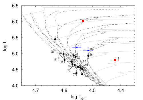
Note that though we interpret these $\dot{M}$ as upper limits, the automated fitting method did return a best fit value. Figure 8 shows the strength of the stellar winds of our entire sample in terms of the modified wind momentum (see Sect. 4.6 for a discussion). The inverted triangles represent upper limits. All these upper limits are well above (up to two orders of magnitude) the mass loss rates derived on the basis of UV profile fitting; not a single one “by chance” gives a value comparable to what is found with the UV method. Why is this so? We can identify two potential reasons. First, the automated fitting procedure scans the mass loss dimension in a linear way. For weak wind cases typical lower and upper bounds of this dimension are $10^{-9}$ and $10^{-7}$ $M_{\sun}{\rm yr}^{-1}$. In most cases it is reasonable to assume that only above $10^{-7}$ $M_{\sun}{\rm yr}^{-1}$ the profile of H$\alpha$ is sensitive to mass loss. In that case it is, e.g. nine times as likely that the automated method more-or-less by chance settles for a mass loss above $10^{-8}$ $M_{\sun}{\rm yr}^{-1}$, and not for the much lower values indicated by UV analysis. Second, small errors in the broadening function of H$\alpha$ may perhaps be “corrected” in the automated fitting process by settling for a mass loss which is “as high as possible”. Consequently, we conclude that we cannot assign any importance to the best fit value returned by the automated method when the downward errors extend to the lower bound of $\dot{M}$ allowed in the fitting process.

7 On the evolutionary status of NGC 346

Undoubtedly the large number of early-type stars in NGC 346 (Massey et al., 1989) is indicative for a young age. Further evidence for the youthful nature of this cluster may be given by the presence of several so-called Vz stars, which are hypothesised to represent the earliest stages of main sequence evolution of massive stars (e.g. Walborn & Parker, 1992; Parker et al., 1992). In this section we will determine an age estimate for NGC 346 and try to quantify the uncertainty rotation introduces in this estimate. We will also discuss how well the spectroscopic Vz designation correlates with ZAMS evolution.

7.1 The age of NGC 346

Rotation affects both the lifetimes and the tracks of stellar evolution models. Consequently, before we can estimate the age of NGC 346 we need to assess the systematic uncertainty rotation will introduce in the age estimate. We do this by considering the differences between isochrones derived from the non rotating models of Charbonnel et al. (1993) and those based on the rotating models of Maeder & Meynet (2001) and Meynet & Maeder (2005) adopting an initial $v_{\rm r}$ of 300 km s^-1. In Fig. 13 the two sets are shown as, respectively, dashed and dotted curves for zero age, 1, 2, 3, 4, 5 and 7 Myr. For reference the evolutionary tracks of the models accounting for rotation are also shown in this figure using grey lines.

Age determinations of individual stars, based on the evolutionary tracks, are given in Fig. 14. The error bars on these life times account for the uncertainties in temperature and luminosity. Open symbols (see the figure caption for details) refer to non-rotating tracks; grey symbols for those accounting for rotation. Note that they differ only very modestly for relatively unevolved objects. For instance, stars near the main sequence are judged to be $\sim$$10^{5}$ years younger if rotation is taken into account. We estimate that for main sequence stars having luminosities larger than $\log\mbox{$L_{\star}$}/\mbox{$L_{\sun}$}\approx 4.5$ this systematic difference may increase up to approximately 0.5 Myr. For the more evolved phases, i.e. approximately giant phase and later, this systematic discrepancy switches sign and rapidly becomes larger. Considering the supergiant NGC 346-001 at $\log\mbox{$L_{\star}$}/\mbox{$L_{\sun}$}=6.0$ we estimate its age to be $\sim$1 Myr more if it is initially rotating with $\mbox{$v_{\rm r}$}\sim 300\mbox{km\,s${}^{-1}$}$ compared to the non-rotating case.

Ignoring the supergiant NGC 346-012 at $\log\mbox{$T_{\rm eff}$}\approx 4.4$, for which cluster membership is very uncertain (Evans et al., 2006), we find that the objects populate the region between the ZAMS and the 7 Myr isochrone, with typical error bars (in both directions) of 2–5 Myr.

So, what could explain the apparent age scatter? First, some objects in our sample might actually not belong to the cluster. In addition to NGC 346-012 this is, for instance, also suggested by Walborn et al. (2000) for the B0 dwarf NGC 346-026. Based on its spatial location, discrepant radial velocity and stellar parameters these authors conclude that this object is not a coeval member of the cluster. Its large age of about 7 Myr seems to support this conclusion. Because of cluster membership issues we have placed both NGC 346-012 and NGC 346-026 to the right in Fig. 14 and have separated them from the other stars using a vertical dashed line. For the remainder of the discussion we treat them as not belonging to the cluster. Second, the Oe star NGC 346-018 is poorly fitted because of contamination by circumstellar material. This implies that the parameters derived for this star should be taken with considerable care, and therefore also the apparently large age of about 7 Myr that we derive for this object. Ignoring the above three discussed objects the oldest investigated star in NGC 346 is $\sim$ 5 Myr (NGC 346-010).

Figure 14: Age determination of the programme stars in NGC 346 using the non-rotating SMC models of Charbonnel et al. (1993) (open symbols) and those including rotation (Maeder & Meynet, 2001; Meynet & Maeder, 2005) (closed symbols). Circles, triangles, and squares denote dwarfs, giants, and supergiants, respectively. The horizontal axis gives the ID number of the star (see e.g. Tab. 3); the vertical axis the age in Myr. The lower limits (upwards pointing arrows) provide age estimates from tracks of chemically homogeneous evolution (Yoon et al. in preparation); see text for a discussion.

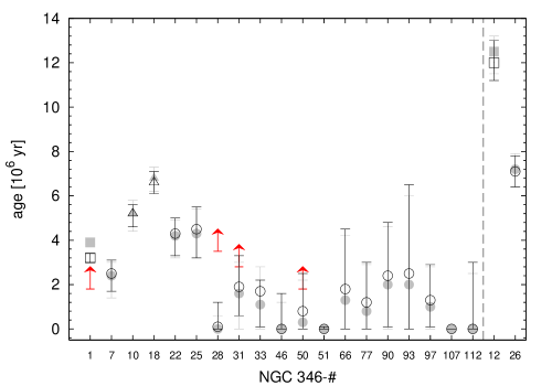
What remains is an age spread of stars from zero to the above motivated 5 Myr. Can such an age spread be explained? We first checked whether there is a relation between the age of the stars and their distance to the cluster centre. Though we do see that the oldest stars (NGC 346-001 through NGC 346-025) are all at some distance from the centre this also holds for some that are assigned very young ages. Also two relatively old stars (NGC 346-007 and NGC 346-022) are located relatively close to the cluster core. Therefore, we can not claim such a relation.

Next we consider the possibility that the adopted tracks are not appropriate for some stars. As we have explained, when it comes to age determination there is no fundamental difference between tracks without rotation and those that do account for it starting the evolution from an initial $v_{\rm r}$ = 300 km s^-1. However, as already discussed in Sect. 4.4, if $v_{\rm r}$ exceeds some critical value the evolution will show a bifurcation behaviour, leading to tracks that evolve bluewards (from the ZAMS) and upwards. This is the result of such efficient mixing that the HRD behaviour proceeds as for chemically homogeneous evolution. Adopting such tracks from Yoon et al. (in prep.) (also see Yoon & Langer, 2005) it turned out to be difficult to derive ages as for near critical rotation the effective temperature changes so rapidly (as a function of $v_{\rm r}$) that one can in practise only rely on luminosity as an age discriminator. Given the error bars on $L$ and $M_{\rm s}$ this did not lead to meaningful constraints for most of the objects. Moreover, in a few cases the mass discrepancy turned out to be so large that the luminosity range implied by $M_{\rm s}$ (plus errors) did not coincide with the observed $L_{\star}$. This also prevents one from deriving an age estimate.

A different approach we tried is based on the fact that for chemically homogeneous evolution the surface helium abundance is essentially a measure of stellar age, for given initial mass. Taking into account the errors on $Y_{\rm He}$ and $M_{\rm s}$, this may yield lower limits to the age of the stars. One derives lower limits because if evolution is not fully chemically homogeneous the measured helium abundance is a lower limit for the mean stellar $Y_{\rm He}$. The method will only provide useful results for those stars that show enhanced helium even when correcting for the negative error in $Y_{\rm He}$. This is the case for four objects (NGC 346-001, NGC 346-028, NGC 346-31, and NGC 346-050). The derived lower age limits are shown in Fig. 14 (arrow symbols). The lower limit of NGC 346-001 (the most massive star) is consistent with the age as derived using the standard method. Interestingly, the lower limits of the ages of the three remaining stars are all significantly above what we derived using modestly rotating or non-rotating models. We have no indication that our $Y_{\rm He}$ determinations are flawed or that these stars had an initial helium fraction significantly higher than 0.09. Consequently, it is likely that these stars evolve along chemically homogeneous tracks and have ages comparable to the oldest stars in the cluster.

In view of the above discussion we have to conclude that we can not derive a unique age for NGC 346. The distribution of ages seems to indicate two preferred values: 1–3 Myr and 3–5 Myr. We add that some stars appear to reside on or even to the left of the ZAMS. Though, it could be that these latter stars evolve along tracks for rapidly rotating stars (following tracks for chemically homogeneously evolving stars). If so, we could not constrain their ages from such models. The ages estimated from modestly rotating or non-rotating evolutionary models of three helium enriched dwarf objects are so low (less than 2 Myr) that it is not possible to bring them into agreement with the derived $Y_{\rm He}$ values. Chemically homogeneous evolutionary models instead predict an age comparible with the oldest cluster population. Given/assuming that all stars belong to the same compact cluster it seems very unlikely that the range of ages implies that NGC 346 experienced a prolonged burst of star formation, or a series of short bursts resulting in multiple coeval populations.

The age of NGC 346 was also estimated by Kudritzki et al. (1983), Massey et al. (1989), Walborn et al. (2000) and Bouret et al. (2003) (also see Massey et al., 2005). In the first, second and fourth studies ages of 2.6 Myr, 2–4 Myr and 3 Myr were found, which in principle are consistent with our findings. Walborn et al. estimate an age of only 1 Myr. This agrees with our lower age limit. The reason for their young age estimate is that their four star NGC 346 sample predominantly contained the stars in the cluster closest to the ZAMS. Combined with the $T_{\rm eff}$ calibration from Vacca et al. (1996) adopted by these authors, which resulted in relatively high estimates for this parameter, for instance, compared to the analysis of Bouret et al. (2003), explains their relatively young age estimate.

7.2 ZAMS stars

The defining characteristic of the luminosity class designation Vz is a very intense He ii $\lambda$4686 absorption line that is substantially stronger than any of the other helium absorption lines. The distinct behaviour of this line is believed to be linked to a luminosity effect connected to an early evolutionary phase. As Vz stars are hypothesised to lie relatively close to the ZAMS they are anticipated to be less luminous compared to normal dwarf stars. As a result of this, the relatively strong $\lambda$4686 line can be explained as a lack of partial filling in of the line profile due to (wind) emission which normal dwarf stars do experience (Parker et al., 1992; Walborn & Blades, 1997).

In the HR-diagram shown in Fig. 13 we have highlighted the location of the three NGC 346 Vz stars in our sample using grey circles. From these three objects, NGC 346-028, NGC 346-031 and NGC 346-051, we find that the first and last are indeed found to lie on or left of the ZAMS. NGC 346-031 in contrast occupies a location between the one and two million year isochrones. We suspect that that the strong He ii $\lambda$4686 line in the spectrum of this object is in fact related to its peculiar chemical composition (see Sect. 4.4). Moreover, the spatial separation of NGC 346-031 of $\sim$5 arcminutes from the cluster centre, makes it unlikely that this object is formed recently as part of the cluster. Consequently, care should be taken with the correct interpretation of Vz stars as near-ZAMS objects, based on optical classification criteria only.

In addition to the two Vz stars Fig. 13 reveals the presence of three more stars located on or left of the ZAMS. Even though the spectra of these objects, NGC 346-046, NGC 346-107 and NGC 346-112, do not exhibit the Vz characteristics, their location in the HR-diagram clearly suggest an early evolutionary phase. Why is this so? We suspect that the reason for the lack of a strong He ii $\lambda$4686 line in the spectra of these objects is related to their relatively low effective temperatures. Compared to the neutral helium lines the relative strength of the He ii lines decreases for decreasing $T_{\rm eff}$. Consequently, even though its line profile is not filled in it becomes more unlikely for the He ii $\lambda$4686 to be stronger than all the He i lines for relatively low effective temperatures. In Fig. 13 we see that these normal dwarf stars are indeed cooler than the Vz stars at the ZAMS. Interestingly, it turns out that in the spectrum of the hottest of these three objects, NGC 346-046, the He ii $\lambda$4686 is the strongest He ii line, which has a strength that is approximately equal to the strength of the strongest He i line. We therefore argue that the effective temperature of this object, i.e. $\sim$40 kK, corresponds to the lower limit of $T_{\rm eff}$ for SMC metallicity for which a Vz luminosity class designation is at all possible.

8 Summary and conclusions

Using the automated fitting method developed by Mokiem et al. (2005), which combines the stellar atmosphere code fastwind with the genetic algorithm based optimisation routine pikaia, we have performed a quantitative analysis of 31 O- and early B-type stars located in the SMC. This sample was mostly drawn from the targets observed in the SMC clusters NGC 346 and NGC 330 as part of the VLT-FLAMES survey of massive stars (see Evans et al., 2005), and is the largest sample of early-type SMC stars analysed so far. Even though many of the observed spectra show nebular contamination and have signal-to-noise ratios as low as 50, the fitting method did not encounter convergence problems. Instead we find that the quality of the data is naturally reflected in the errors that are estimated for the fit parameters using the width of the global optimum.

Concerning the stellar properties of the objects in our sample we can draw the following conclusions:

1. The average effective temperature for a given spectral type for SMC dwarf stars is hotter by typically 3 to 4 kK than for their Galactic counterparts (Martins et al., 2005a). We attribute this hotter temperature scale to a reduced line blanketing in the SMC. In contrast to Massey et al. (2005) we find that this blanketing effect on $T_{\rm eff}$ extends to spectral types as late as B0.

2. The helium enrichment found in our stars does not appear to be consistent with predictions of the evolution of massive stars ignoring rotation. Comparison with evolutionary tracks that do account for rotation shows a qualitative agreement. In the HR-diagram the region in which a helium enrichment is predicted roughly coincides with the location of evolved objects showing evidence of $Y_{\rm He}$ enrichment. The actual degree of enrichment is in many cases still strongly under predicted by the most recent evolutionary models.

3. From our three programme stars with a Vz luminosity class designation, we find that only two are true ZAMS objects. Moreover, three additional objects, which are not classified as Vz stars, are found to lie on or left of the ZAMS. We argue that this is related to a temperature effect inhibiting relatively cool stars located on the ZAMS to exhibit the spectral features characteristic for the Vz luminosity class.

4. We find good agreement between our spectroscopically derived masses and those derived from evolutionary calculations. A mild mass discrepancy is still found for stars with $\mbox{$M_{\rm s}$}\lesssim 20\,\mbox{$M_{\sun}$}$. This discrepancy correlates with the surface helium abundance and is qualitatively consistent with the predictions of chemically homogeneous evolution.

The stars in the young cluster NGC 346 allow to study the role of mass loss and angular momentum loss during the early evolution of massive stars in a low metallicity environment. Regarding these issues we can conclude that:

1. The observed distribution of $v_{\rm r}\sin i$ for evolved stars (luminosity classes I-II) contains relatively less fast rotators and slow rotators compared to the distribution for unevolved stars (luminosity classes IV-V). These findings are in agreement with analyses of Galactic samples and can be interpreted as a spin down due to an increased radius and angular momentum loss through the stellar wind, and excess turbulent broadening among the evolved stars (cf. Howarth et al., 1997). We also find that compared to the velocity distribution of unevolved Galactic objects the distribution for unevolved SMC objects shows a relative excess of stars rotating with projected velocities $120\gtrsim\mbox{$v_{\rm r}\sin i$}\lesssim 190\,\mbox{km\,s${}^{-1}$}$. This excess can be interpreted as evidence of a reduction of dissipation of angular momentum in weaker stellar winds resulting from the low $Z$ environment of the SMC.

2. Using a simple modelling approach we have constrained the underlying $v_{\rm r}$ distribution of the unevolved SMC stars. The exact shape of this underlying distribution – for which we have tried a block, Gaussian and Maxwellian shape – is found to be degenerate, however, it can be characterised by a mean velocity of about $150-180$ km s^-1 and an effective half width of roughly $100-150$ km s^-1. The Maxwellian distribution appears a somewhat poorer representation of the $v_{\rm r}$ distribution, indicating that 5–15 percent of the stars must be slow rotators ($\mbox{$v_{\rm r}$}\lesssim 50$ km s^-1).

3. It is not possible to derive a unique age for NGC 346 using moderately rotating or non-rotating evolutionary models. Though the bulk of the stars indicate a lifetime of 1–3 Myr, part of the investigated stars seem somewhat older (3–5 Myr). Clearly the ages depend on the adopted evolutionary tracks. However, we point out that predictions for non-rotating stars and those accounting for the rotational evolution of stars with an initial $\mbox{$v_{\rm r}$}=300$ km s^-1 essentially give the same result. Three main sequence stars, all with an age determination of less than 2 Myr, show significant helium enhancement. Assuming that these stars have the same initial $Y_{\rm He}$ this implies a lower limit to their age of 2 to 3.5 Myr.

4. Based on the predictions of the time evolution of the equatorial velocity for low metallicity (Maeder & Meynet, 2001) the above age considerations imply that the underlying $v_{\rm r}$ distribution derived for our sample (conclusion vi) is representative for the initial rotational velocity distribution.

5. Mass loss rates determined for the SMC objects are found to be systematically lower than for Galactic objects. For $\log\mbox{$L_{\star}$}/\mbox{$L_{\sun}$}\gtrsim 5.4$ we find that the wind strengths are in excellent agreement with the theoretical predictions of Vink, de Koter, & Lamers (2001). The empirical modified wind momentum luminosity relation constructed for this luminosity regime agrees to within the error bars with the predicted WLR.

6. Down to $\log\mbox{$L_{\star}$}/\mbox{$L_{\sun}$}\approx 5.3$ the mass loss rates determined from the optical spectra are in agreement with UV rates. For luminosities lower than this value the winds become too weak for an accurate determination of $\dot{M}$ from the optical spectrum only. Consequently, we cannot (yet) conclude whether or not the UV and H$\alpha$ diagnostics agree or disagree in weak wind situations.

Appendix A Fits and comments on individual objects

The observed spectra shown in this section were corrected for radial velocities. If not noted differently the lines that were fitted are the hydrogen Balmer lines H$\alpha$, H$\gamma$ and H$\delta$; the He i singlet line at 4387 Å; the He i triplet lines at 4026, 4471 and 4713 Å; and the He ii lines at 4200, 4541 and 4686 Å. In general we find that all lines could be fitted quite accurately including the He i $\lambda$4471 for which we only encountered the “generalised dilution” in one case. This is in accordance with the fact that the majority of the sample consists of dwarf stars and the single star where this problem is present, AzV 372, is a late type supergiant.

Figure 15: Comparison of the observed line profiles of NGC 346-001, -007, -010 and -012 with best fitting synthetic line profiles obtained using the automated fitting method (grey lines). Wavelengths are given on the horizontal axis in Å. The vertical axis gives the normalised flux. Note that this axis is scaled differently for each line.

Figure 16: Same as Fig. 15, however, for NGC 346-018, -022, -025 and -026.

Figure 17: Same as Fig. 15, however, for NGC 346-028, -031, -033 and -046.

Figure 18: Same as Fig. 15, however, for NGC 346-050, -051, -066 and -077.

Figure 19: Same as Fig. 15, however, for NGC 346-090, -093, -097 and -107.

Figure 20: Same as Fig. 15, however, for NGC 346-112, NGC 330-031 and -052.

Figure 21: Same as Fig. 15, however, for AzV 14, 15, 26 and 95.

Figure 22: Same as Fig. 15, however, for AzV 243, 372, 388 and 469. Shown with a dotted line for AzV 372 is the effect of an increase of the mass loss rate by 0.1 dex on the line profiles of H$\alpha$ and He ii $\lambda$4686.

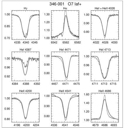
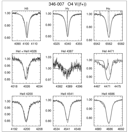
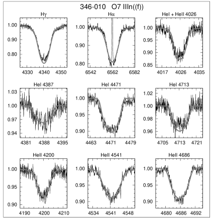
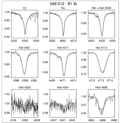
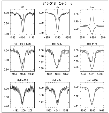
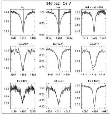
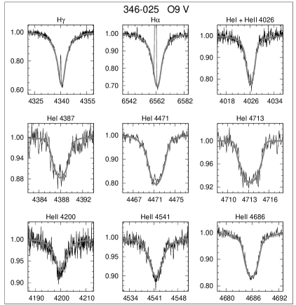
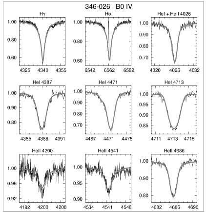
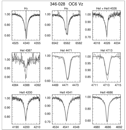
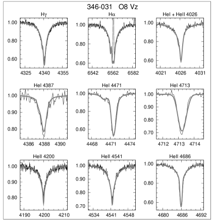
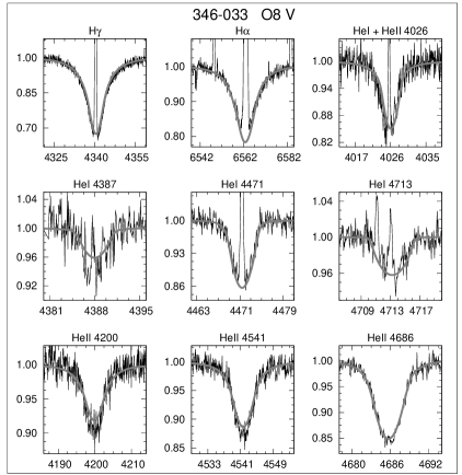
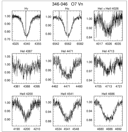
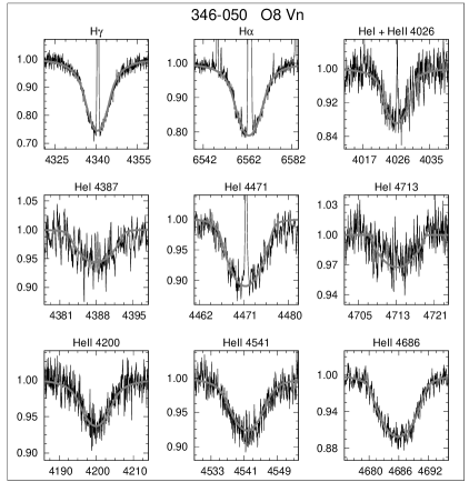
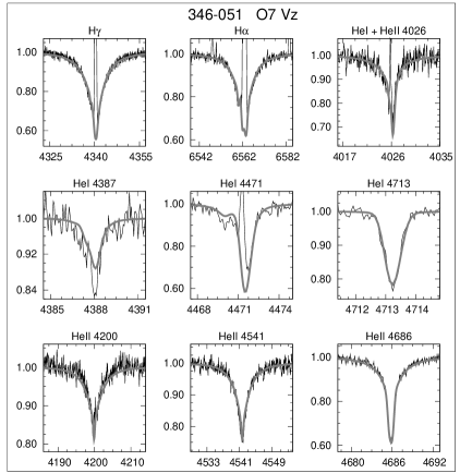
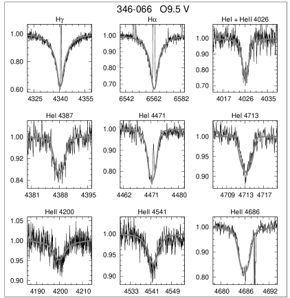
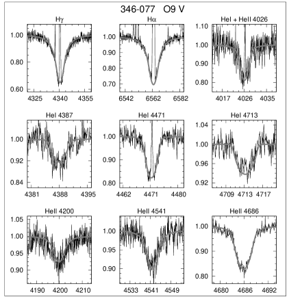
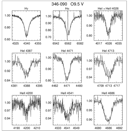
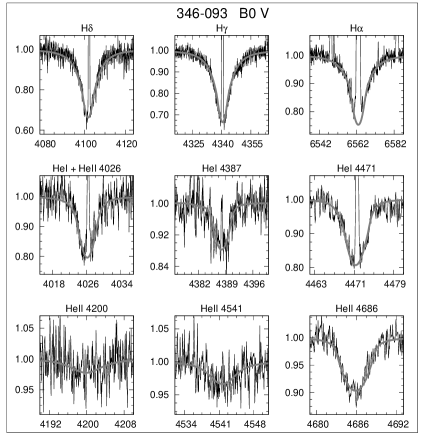
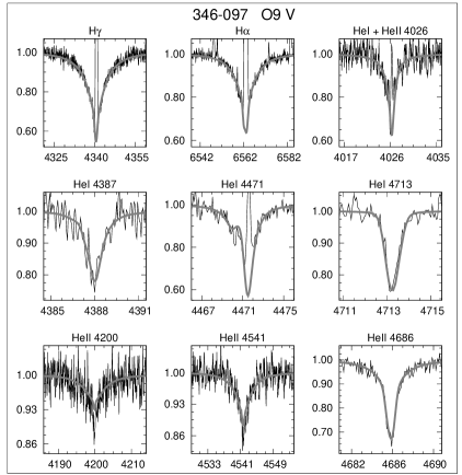
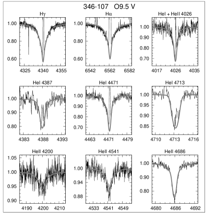
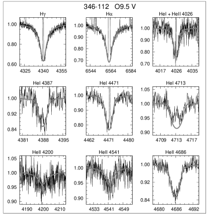
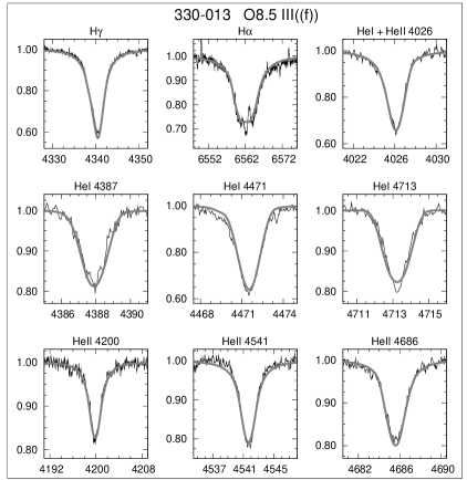
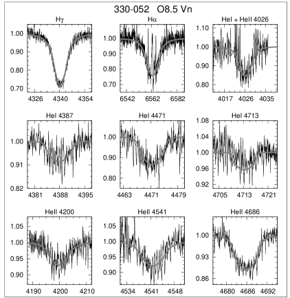
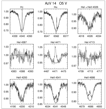
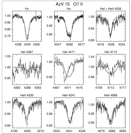
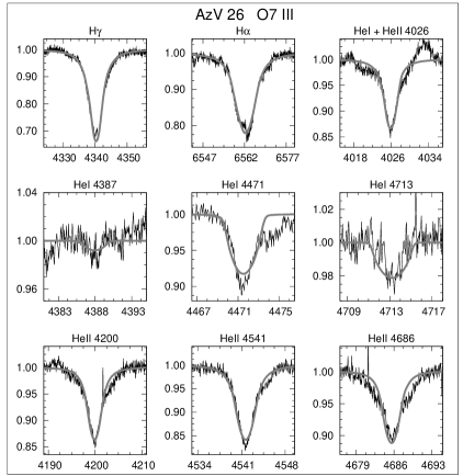
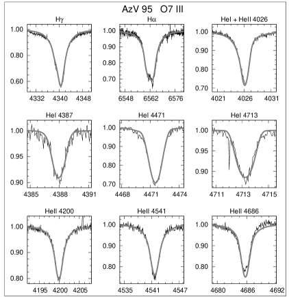
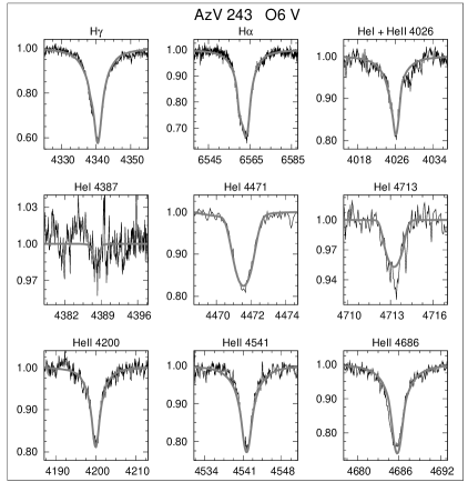
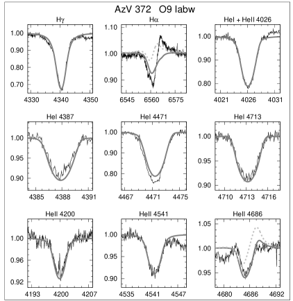
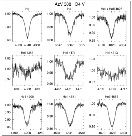
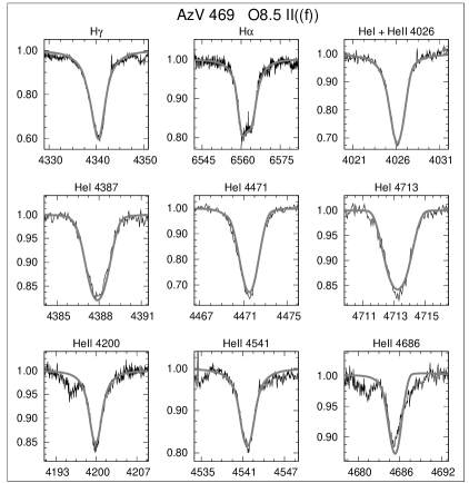
NGC 346-001

The fit of the spectrum of this O7 supergiant is presented in Fig.15. All lines except He i $\lambda$4387 are reproduced well. Note that the nebular contamination on top of the H$\alpha$ line core was disregarded in the fit. The inaccurate reproduction of He i $\lambda$4387 is the result of the low weight given to this line in our weighting scheme (see Paper I). For this low weight the quantitative fit quality of He i $\lambda$4387 is comparable to that of He i $\lambda$4026. Therefore, the discrepancy is not significant and merely reflects the uncertainty with which we believe that the stellar atmosphere code can reproduce this line.

This object was previously studied by Crowther et al. (2002) using the alternative wind code cmfgen (Hillier & Miller 1998). We find good agreement between the photospheric parameters. Note that the helium abundance $\mbox{$Y_{\rm He}$}=0.2$ adopted by Crowther et al. is in good agreement with the $\mbox{$Y_{\rm He}$}=0.24$ self consistently determined here. The largest difference is found for the effective temperature (2 kK). This difference can be explained by the higher surface gravity obtained from our fit, which requires a higher $T_{\rm eff}$ to obtain the same helium ionisation equilibrium. This occurs in many of the fits discussed here, and we attribute this to a better multidimensional parameter optimisation by the automated method. This assures that the global optimum in parameter space is found avoiding $\log{{g}}$ and $T_{\rm eff}$ values which could correspond to a local optimum (see Sect. 5.2 of Paper I).

The mass loss rate obtained from our fit of the optical spectrum is within the error bars in agreement with the value that Crowther et al. derived from the UV spectrum. With respect to the acceleration of the wind we find a large difference. From the optical spectrum we derive $\beta=1.15$, whereas Crowther et al. find $\beta=1.65$ based on the UV resonance lines. They do note that from their modelling of H$\alpha$ they obtain a smaller value for this parameter, indicating a possible systematic discrepancy between wind accelerations determined from optical and UV spectra (also see Puls et al. 1996).

NGC 346-007

With exception of the He i line at 4471 Å, which suffers from very strong nebular contamination, a good fit was obtained for this object. Note that the fit shown in Fig. 15 does not include the He i 4713 line. The nebular contamination in this line proved to be too severe to obtain a reliable fit.

Within the uncertainties the photospheric parameters $T_{\rm eff}$ and $\log{{g}}$ are in good agreement with those of Bouret et al. (2003) who used cmfgen for their analysis. These authors find $\mbox{$T_{\rm eff}$}=41.5$ kK and $\mbox{$\log{{g}}$}=4.0$. The automated method was not able to self consistently derive $\beta$. Consequently, a fixed value of $\beta=0.8$ was used. With this fixed value a mass loss rate of $2.3\times 10^{-7}\,\mbox{$M_{\sun}{\rm yr}^{-1}$}$ is found, which is also in good agreement with the rate derived by Bouret et al. from a fit to the wind sensitive UV lines.

The effective temperature of $\mbox{$T_{\rm eff}$}=42.8$ kK obtained here is in poor agreement with the recent analysis of Heap et al. (2006). Using the plane-parallel atmosphere model tlusty these authors derive a relatively low $T_{\rm eff}$ of 40 kK. The reason for this discrepancy is unknown, but can probably be attributed to a different treatment of line blanketing in tlusty and fastwind, or the coarsely sampled grid of models used by Heap et al.

NGC 346-010

is a fast rotator. To obtain the fit displayed in Fig. 15 a projected rotational velocity of 313 km s^-1 was needed. Even though all lines seem to be fitted correctly we note a slight over prediction of the strength of the wings of the wind sensitive He ii $\lambda$4686 and H$\alpha$ lines. The shape of the former line could indicate the existence of denser equatorial material or possible the presence of a disk.

NGC 346-012

As can be seen in Fig. 15 the low projected rotational velocity of this B-supergiant allowed for a nearly perfect fit. Note that given the relative scaling of the plots in Fig. 15 the fit quality of the He ii lines is similar to that of the neutral helium lines, i.e. they are fitted well.

The good fit quality obtained resulted in relatively small error estimates (cf. Tab. 4). Most interestingly, the uncertainties on the wind parameters, considering the very tenuous wind of this object, are modest as well. This is mostly because H$\alpha$ is not affected by nebular contamination. As a result of this the strength and the shape of this wind sensitive line could be matched very accurately with little room for error.

NGC 346-018

The line profiles of this object suffer from strong contamination, making it problematic to obtain a good fit. We believe that this emission is not only nebular in origin, but, given the breadth in the hydrogen lines, is possibly also emitted from a circumstellar disk. The contamination in the H$\alpha$ Balmer line proved so severe that we did not include it in the fitting process. Our best fitting model is presented in Fig. 16.

NGC 346-022

A good quality fit was obtained for this object. The nebular emission in the core of the He i 4471 line did not hamper an accurate determination of the effective temperature, hence the small error given in Tab. 4. This $T_{\rm eff}$ is considerably larger than the effective temperature one would expect for a Galactic O9 dwarf (see Martins et al. 2005a). However, it is in line with the expectation of a reduced line blanketing effect as a result of a low Z environment, and is in agreement with the values obtained for the other O9 V stars in our sample (see Sect. 4.1).

Heap et al. (2006) determined a relatively low $T_{\rm eff}$ of 32.5 kK for this object, which is a consequence of the low surface gravity of $\mbox{$\log{{g}}$}=3.75$ determined by these authors. In contrast the automated method obtained $\mbox{$\log{{g}}$}=4.2$ requiring a higher $T_{\rm eff}$ to obtain the correct helium ionisation equilibrium.

NGC 346-025

The parameters obtained for this object are very similar to the parameters used to fit the previously discussed object. The only difference is in the projected rotational velocity, which is higher by more than a factor of two.

NGC 346-026

All lines, including the weak He ii lines, are fitted well for this object. In the Fig. 16 the final fit is presented. The luminosity classification IV ascribed to this object is reflected in the gravity of $\mbox{$\log{{g}}$}=3.76$. This value is still higher by 0.16 dex compared to the value determined by Bouret et al. (2003) and Heap et al. (2006). Accordingly, the $T_{\rm eff}$ determined by the automated method is also higher by 1.1 kK.

NGC 346-028

This object is classified as an OC6 Vz star, indicating that its spectrum shows signatures of a relatively low nitrogen abundance and evidence for an early evolutionary state. Evidence for the latter is provided by the large relative strength of the He ii $\lambda$4686 line (also see Sect. 7.2). In Fig. 17 the best fit is presented. Note how well the He ii blends in the hydrogen lines are reproduced. The effective temperature and luminosity place this object at a position close to the ZAMS in the HR-diagram shown in Fig. 13, corroborating its young age.

Compared to the analyses of Bouret et al. (2003) and Heap et al. (2006) we find an effective temperature higher by almost 3 kK. This is likely related to the large helium abundance we found. In contrast, Bouret et al. and Heap et al. adopted the Solar value for this parameter. In terms of the wind parameters we were only able to determine an upper limit of $10^{-7}\,\mbox{$M_{\sun}{\rm yr}^{-1}$}$ which is at least consistent with the $3\times 10^{-9}\,\mbox{$M_{\sun}{\rm yr}^{-1}$}$ derived by Bouret et al. from the UV spectrum.

NGC 346-031

is also classified as a Vz type object. The fit to its spectrum is shown in Fig. 17. In contrast to NGC 346-028 the location of this object in the HR-diagram does not corroborate its youthful spectral classification. Instead the isochrones suggest an age of 1–2 Myr.

NGC 346-033

The fit presented in Fig. 17 shows that despite the strong nebular contamination in the neutral helium lines, a good fit could be obtained for this O8 dwarf. The best fit mass loss rate of $7.4\times 10^{-7}\,\mbox{$M_{\sun}{\rm yr}^{-1}$}$ seems rather high for its luminosity. The reason for the large $\dot{M}$ is likely the anomalously large wind velocity ($\sim$4100 km s^-1), which resulted from a scaling with the escape velocity at the stellar surface (see Sect. 4.6).

NGC 346-046

The shape of the line profiles of this object are indicative for fast stellar rotation. This is confirmed by the fit shown in Fig. 17, for which a $v_{\rm r}\sin i$ of 340 km s^-1 was needed, classifying 346-046 as a very fast rotator. The helium abundance is slightly enhanced, which could be related to the rapid rotation of this object. However, one has to keep in mind that the error estimate on this parameter is of the same order of the enrichment, when considering this statement.

NGC 346-050

To fit the line profiles, displayed in Fig. 18, a $v_{\rm r}\sin i$ of 357 km s^-1 was needed. Interestingly, similar to the other fast rotator 346-046 a small helium enhancement was found.

NGC 346-051

is the final Vz object in our sample. Its spectrum suffers from strong nebular contamination. Nevertheless a good fit could be obtained, which is presented in Fig. 18. The location of NGC 346-051 in the HR-diagram presented in Fig. 13 points to an early evolutionary phase for this object.

NGC 346-066

The line profiles of this object are matched well by the synthetic profiles. In the final fit, shown in Fig. 18, only the He i line at 4713 Å shows a slight mismatch due to an apparent over prediction of the width of this line. Given the signal-to-noise ratio of the spectrum, we do not believe this to be significant.

NGC 346-077

A good fit was obtained despite the strong nebular contamination affecting the hydrogen and neutral helium lines. The final fit is displayed in Fig. 18.

NGC 346-090

Like 346-066 this object is of spectral type O9 V. The fit to its spectrum is presented in Fig. 19. Compared to 346-066 a $T_{\rm eff}$ lower by $\sim$800 K was obtained. This is the result of the weaker He ii lines.

NGC 346-093

The fit to the spectrum of the B0 dwarf NGC 346-093 is shown in Fig. 19. This fit shows that the very weak He ii lines at 4200 and 4541 Å could still be fitted using the automated method.

NGC 346-097

The final fit to the spectrum of the O9 dwarf 346-097 is presented in Fig. 19. Even though the nebular emission is quite severe in the hydrogen lines and in some of the helium lines a good fit was obtained. Its parameters are in agreement with other O9 V objects in our sample. Note that the gravity of $\mbox{$\log{{g}}$}=4.5$ is remarkably high.

NGC 346-107

The nebular contamination, as shown in Fig. 19, is severe in the spectrum of this object. All hydrogen and neutral helium lines suffer from nebular emission. This did not prevent the automated fitting method from obtaining a reliable fit. Most importantly, the effective temperature, determined without information about the cores of the He i lines, is in good agreement with the other O9.5 V objects studied here.

NGC 346-112

The spectrum of 346-112 is rather noisy, which is the result of its low luminosity of $\log L=4.36\leavevmode\nobreak\ \mbox{$L_{\sun}$}$, making it the intrinsically faintest object in our sample. Also strong nebular contamination is present in the line cores. The fit to the spectrum is presented in Fig. 20. Despite the low quality of the data the fits of the line profiles are good. The low S/N value does, however, result in large error bars (cf. Tab. 4).

NGC 330-013

As can be seen in Fig. 20 all lines of this O8.5 giant could be fitted accurately. In the HR-diagram in Fig. 6 this object is found to lie close to the region in which rotating evolutionary models predict a helium surface enrichment. The relatively high helium abundance of $\mbox{$Y_{\rm He}$}=0.18$, which was needed to obtain this fit, seems to be in agreement with rotationally enhanced mixing effects (see Sect. 4.4).

NGC 330-052

Presented in Fig. 20 is the spectrum of NGC 330-052. The H$\delta$ Balmer line was not fitted as the spectrum around in that region was of a too low quality. Despite this missing line and the low signal-to-noise ratio, a good fit could be obtained. The low quality of the spectrum does result in relatively large error estimates (cf. Tab. 4).

AzV 14

For this object and the remaining objects the hydrogen Balmer line H$\beta$ was also fitted. The spectrum of the O5 V star suffers from strong nebular contamination in both the He i and He ii lines. However, the fit shown in Fig. 21, does seem to reproduce the observed features correctly. A comparison with the parameters determined by Massey et al. (2004), who also used fastwind, confirm this. Within the error bars the parameter values are comparable.

AzV 15

The He i $\lambda$4471 line in the spectrum shown in Fig. 21 is strongly affected by nebular emission. This hampers an accurate determination of the effective temperature and the surface gravity, which is reflected in relatively large error estimates listed in Tab. 4. Nebular emission can also introduce a systematic error in the determination of these parameters. However, the behaviour of this object in the $T_{\rm eff}$ vs. spectral type diagram and log $T_{\rm eff}$– $\log{{g}}_{\rm c}$ plane does not indicate a problem. Moreover, a “normal” helium abundance of $\mbox{$Y_{\rm He}$}=0.10$ is recovered from the spectrum, indicating that the He i line profiles contain enough information to avoid a degeneracy effect between $T_{\rm eff}$ and $Y_{\rm He}$ (also see Paper I). All in all, we conclude that despite the strong nebular contamination the parameters of AzV 15 are robust. This conclusion is strengthened by the good agreement between the projected rotational velocity we determine from the optical (135 km s^-1) and the value determined by Penny et al. (2004). These authors used cross-correlation techniques to determine $\mbox{$v_{\rm r}\sin i$}=128\leavevmode\nobreak\ \mbox{km\,s${}^{-1}$}$ from UV spectra.

Heap et al. (2006) derive a considerably lower $T_{\rm eff}$ of 37 kK. This is connected to the $\log{{g}}$ value obtained by these authors that was lower by $\sim$0.2 dex.

AzV 26

A good fit was obtained for AzV 26, though in the final fit presented in Fig. 21 there is a small under prediction of the line wings of He ii $\lambda$4686. A possible explanation of the latter may be an incorrect projected rotational velocity. However, the value $\mbox{$v_{\rm r}\sin i$}=132\,\mbox{km\,s${}^{-1}$}$ obtained from the automated fit is in perfect agreement with the value of $\mbox{$v_{\rm r}\sin i$}=127\,\mbox{km\,s${}^{-1}$}$ Penny et al. (2004) derived from the UV spectrum. Therefore, this small discrepancy remains unexplained.

Compared to the analysis by Massey et al. (2004) the largest differences are found for $T_{\rm eff}$ and $\log{{g}}$, for which the automated method determined values higher by $\sim$2 kK and 0.25 dex, respectively, and $\dot{M}$, for which a value lower by 0.16 dex was obtained. A small part of the difference in surface gravity can be explained by the larger $v_{\rm r}\sin i$ of 150 km s^-1 adopted by these authors. The largest part of the difference in $\log{{g}}$ and $T_{\rm eff}$ we believe is the result of a better multidimensional parameter optimisation by the automated method (see above). The reduced mass loss rate can be explained by the larger value of $\beta$ found in this study. Massey et al. assumed a fixed value of $\beta=0.8$, whereas we find $\beta=1.17$.

AzV 95

The best fit obtained for this O7 giant is presented in Fig. 21. The accurate reproduction of all lines and the modest error estimates require no further comments. We note that Heap et al. (2006) in their analysis obtained a $T_{\rm eff}$ value that is lower by $\sim$3 kK. We ascribe this difference to the gravity determination of these authors, which was lower by approximately 0.3 dex.

AzV 243

In Fig. 22 the spectrum of AzV 243 is presented. With the automated method we were able to obtain a very good fit for all lines. The final parameters can be compared to the work of Haser et al. (1998). With exception of the effective temperature that Haser et al. adopted from the analysis of Puls et al. (1996) and $\beta$, there is good agreement. Our effective temperature is lower by $\sim$1000 K, which we attribute to the inclusion of line blanketing in our analysis. The acceleration of the wind was determined by Haser et al. to be $\beta=0.7$, based on UV resonance lines. Our value of $\beta=1.4$ was derived from the optical spectrum. The reason for this discrepancy is unclear. However, it could be related to the fact that the wind is very weak (order $10^{-7}$ $M_{\sun}{\rm yr}^{-1}$), introducing a large error in the determination of this parameter.

Compared to the study of Penny et al. (2004) we again find good agreement between our $v_{\rm r}\sin i$ determined from the optical (59 km s^-1) and their $v_{\rm r}\sin i$ derived from a UV analysis (62 km s^-1).

AzV 372

Based on its peculiar H$\alpha$ profile and the fact that they were unable to simultaneously fit the He i and He ii lines Massey et al. (2004) suggest that this object is a spectroscopic binary. However, the fit presented in Fig. 22 shows that a simultaneous fit of both the He i and He ii lines for a single set of parameters is possible. Therefore, we do not concur with the findings of Massey et al. and treat AzV 372 as a single star. Note that we did encounter a mild form of the “generalised dilution” effect in the He i $\lambda$4471 line.

Using our fitting method, reproduction of the H$\alpha$ line still remains difficult. We are not able to satisfactorily match the absorption and the weak emission simultaneously. To fit the emission an increase of $\dot{M}$ of the same order as the error estimate of this parameter is necessary. In Fig. 22 the effect of an increase of the mass loss rate with 0.1 dex on the line profiles of H$\alpha$ and He ii $\lambda$4686 is shown using a dotted line. Consequently, given the modest increase in $\dot{M}$ required we regard our determination of the mass loss rate as correct within the given error estimates.

AzV 372 was also analysed by Evans et al. (2004a). Compared to this study we find differences for $T_{\rm eff}$, $Y_{\rm He}$, $\dot{M}$ and $\beta$. The effective temperature from the automated method is larger by approximately 3 kK. This is probably linked to the reduced helium abundance we find and the improved fit of the He ii lines (e.g. see Fig. 3 of Evans et al.). Our mass loss rate is approximately a factor of two larger than the $\dot{M}$ determined by Evans et al.. We can explain this difference by the large $\beta$ these authors derive. To match the H$\alpha$ profile Evans et al. needed $\beta=2.25$, whereas we obtained $\beta=1.27$ using the automated method. As a larger value for $\beta$ results in a slower accelerating wind and, consequently, in a higher density in the H$\alpha$ line forming region, the required mass loss rate to reproduce the H$\alpha$ line profile is decreased. Note that our wind parameters, in contrast to Evans et al., can reproduce the He ii $\lambda$4686 line profile correctly. However, one should realise that in our fitting method this line was given a relatively high weight compared to the fit of Evans et al. (2004a), who gave priority to H$\alpha$. Consequently, the differences in wind parameters for this object also reflect the particularly peculiar shape of the wind lines and the difficulties involved in reproducing them.

AzV 388

For the O4 dwarf AzV 388 a good fit was obtained. As is shown in Fig. 22 all line profiles are reproduced accurately. The projected rotational velocity of 163 km s^-1 required to fit the profiles is in good agreement with the UV determination by Penny et al. (2004). They find $\mbox{$v_{\rm r}\sin i$}=179\,\mbox{km\,s${}^{-1}$}$.

AzV 469

The fit to the spectrum of AzV 469 is shown in Fig. 22. For all lines a good fit was obtained. Our fit parameters compare well with the results of Evans et al. (2004a) who studied this object using cmfgen. In contrast we find large differences for $\log{{g}}$, $T_{\rm eff}$ and $\dot{M}$ when comparing our results to the analysis of Massey et al. (2004) who also analysed AzV 469 using fastwind. Note, however, that the differences are likely the result of a not well constrained fit by Massey et al., as these authors had difficulties matching the H$\alpha$ core emission and severely under predicted the strength of the He i $\lambda$4471 line.