COSMOGRAIL: the COSmological MOnitoring of
GRAvItational Lenses

Abstract

Aims. Our aim is to measure the time delay between the two gravitationally lensed images of the $z_{\rm qso}$ = 1.547 quasar SDSS J1650+4251, in order to estimate the Hubble constant H₀.

Methods. Our measurement is based on $R$-band light curves with 57 epochs obtained at Maidanak Observatory, in Uzbekistan, from May 2004 to September 2005. The photometry is performed using simultaneous deconvolution of the data, which provides the individual light curves of the otherwise blended quasar images. The time delay is determined from the light curves using two very different numerical techniques, i.e., polynomial fitting and direct cross-correlation. The time delay is converted into H₀ following analytical modeling of the potential well.

Results. Our best estimate of the time delay is $\Delta t=49.5\pm 1.9$ days, i.e., we reach a 3.8 % accuracy. The $R$-band flux ratio between the quasar images, corrected for the time delay and for slow microlensing, is $F_{\rm A}/F_{\rm B}=6.2\pm 5$ %.

Conclusions. The accuracy reached on the time delay allows us to discriminate well between families of lens models. As for most other multiply imaged quasars, only models of the lensing galaxy that have a de Vaucouleurs mass profile plus external shear give a Hubble constant compatible with the current most popular value (H₀  = 72 $\pm$ 8 km s^-1 Mpc^-1). A more realistic singular isothermal sphere model plus external shear gives H₀ = 51.7${}^{+4.0}_{-3.0}$ km s^-1 Mpc^-1.

1 Introduction

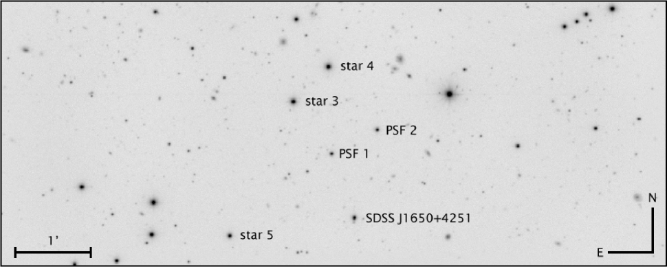
Figure 1: A $R$-band image of SDSS J1650+4251 obtained at Maidanak Observatory. This image is a combination of 376 frames, totalising 31 hours of exposure. The mean seeing is 1.0″, and the field of view is $3.5\arcmin\times 8.9\arcmin$. The two stars labeled PSF1 and PSF2 are used to model the Point Spread Function required for the MCS deconvolution method. The 4 reference stars used for the photometric calibration are star #3, #4, PSF1 and PSF2. Star #5 is used as a cross-check of the deconvolution photometry.

The so-called time-delay method in gravitationally lensed quasars (Refsdal Refsdal64 (1964)) is one of the rare techniques that can yield a measurement of the Hubble constant H₀ at truly cosmological distances, independently of any local calibration or standard candle. Until now, however, no concerted and long-term project has succeeded in applying it in a systematic way, at a level really competitive with other techniques, such as Cepheids, supernovae or the fluctuations of the cosmic microwave background radiation. The COSMOGRAIL project aims at measuring time delays for most known gravitationally lensed quasars, as well as improving their lens models, using deep high resolution imaging and spectroscopy. The contribution of the error on the time delay measurement to the total error budget on H₀ is about 50 %, the other half being due to degeneracies in the lens models. The immediate goal of COSMOGRAIL is to make the former close to negligible in front of the latter. While this is very hard for lenses with short time delays (Kochanek et al. Kochanek06a (2006), Morgan et al. Morgan06 (2006)), longer time delays can be measured accurately (Eigenbrod et al. Eigenbrod05 (2005)).

In this paper, we present the first result from our monitoring program: the time delay measurement in the gravitationally lensed quasar SDSS J1650+4251 (16${}^{\textrm{\scriptsize{h}}}$ 50${}^{\textrm{\scriptsize{m}}}$ 43$\aas@@fstack{s}$5, +42° 51′ 45$\aas@@fstack{\prime\prime}$0; J2000.0), discovered by Morgan et al. (Morgan03 (2003)) as a doubly imaged $z_{\rm qso}$  = 1.547 quasar, with an angular separation of 1.2″. At the time of the discovery, the $B$-band magnitudes of components A and B were $17.8$ and $20.0$ respectively. The lensing galaxy is detected by Morgan et al. (Morgan03 (2003)) in the $I$ band. Absorption lines seen in the spectrum of the quasar images suggest a lens redshift of $z_{\rm lens}$ = 0.577. In a cosmology with H₀ = 75 km s^-1 Mpc^-1, Morgan et al. (Morgan03 (2003)) predict that the time delay between the quasar images is of the order of a month, assuming a Singular Isothermal Sphere (SIS) potential for the lensing galaxy, plus an external shear. Following the non-parametric models of Saha et al. (Saha06 (2006)) and the same cosmology, the expected time delay between the two quasar images is $\Delta t\sim 30-60$ days.

The first two seasons of the photometric monitoring of SDSS J1650+4251 were carried out with the 1.5-m telescope at Maidanak Observatory, in Uzbekistan. Given the high declination of SDSS J1650+4251  and the pointing limits of the telescope, SDSS J1650+4251 can be followed for about 8 months per year under good airmass and seeing conditions. This combination of time delay and visibility window makes SDSS J1650+4251 an excellent target for an accurate time delay measurement. From numerical simulations using artificial light curves, Eigenbrod et al. (Eigenbrod05 (2005)) predict that the accuracy on the time delay can be as good as 1 %, assuming that the peak to peak amplitude of the quasar light variation is 0.2 mag over the two years of observation and using a temporal sampling of at least one observing point per week. Although more than two observing seasons will be necessary to achieve this final goal, it is already possible to measure the time delay with 3.8 % accuracy, which is sufficient to show that lens models with constant mass-to-light ratio and models with dark matter profiles that do not trace light give discrepant values of H₀.

The photometric monitoring, the data reduction and the light curves are presented in Sects. 2 and 3 respectively. The determination of the time delay between the two lensed images is described in Sect. 4. In Sect. 5, we discuss the mass models for the lensing galaxy and the implications for the Hubble constant. Finally, Sect. 6 summarises the main results.

2 Observations

The observations presented in this article consist of two full observing seasons. SDSS J1650+4251  is visible from the end of February to the beginning of October at Maidanak Observatory. The resulting non-visibility window is therefore of about 150 days. Additional, but smaller, gaps are due to bad seeing or weather conditions. The photometric points presented here span a total of 333 days between May 2004 and September 2005, after removal of the non-visibility period. The mean temporal sampling in the visibility window is one point every 5th day.

The CCD camera used at Maidanak Observatory is a 800$\times$2000 array with a pixel size of 0.266″  on the plane of the sky. The useful field of view is 3.5′$\times$8.9′. All data are taken through the Cousins $R$ filter. The seeing varies between 0.7″  and 2.0″  over the two observing seasons, 1.1″ being the most frequent value. For each observing epoch, unless technical or meteorological problem occurs, 6 dithered images are taken. The exposure time for each of the 6 frames is 300 s, and the size of the dithering box is 15″.

3 Reductions and deconvolution

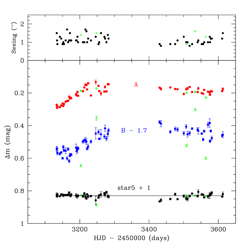
Figure 2: $R$-band light curves for the two quasar images in SDSS J1650+4251, as well as for a reference star in the field of view. The magnitudes are given in relative units. In order to avoid the points overlaps, the component B and the star curves have been shifted in magnitude. The 5 epochs marked by triangles deviate very far away from the otherwise smooth variations of the light curve of component B. They have been removed from the curves when determining the time delay (see Section 4).

The field of view of the camera is shown in Fig. 1, where SDSS J1650+4251 has been slightly off-centered in order to include more stars useful for the construction of the Point Spread Function (PSF). An automated pipeline is used to carry out the pre-reduction of all the individual CCD frames. This pipeline first subtracts a master-bias from each image, then for each night, corrects for the flatfield using twilight flats, and removes a sky-image. The accurate positions of 15 reference stars are then measured on all images with the Sextractor package (Bertin & Arnouts Bertin96 (1996)) and used in IRAF to compute the geometrical transformation between the images. Rebinning of the data using polynomial interpolations is necessary, since rotation and scaling are included in the transformation, in addition to the image shift. We do not perform any cosmic ray removal, since no cosmic ray is present in the tiny field of view considered around SDSS J1650+4251  and around the PSF stars, as indicated by the residual images of the deconvolution.

Since the airmass and the transparency of the sky change with time, cross-calibration of the photometric zero point between all the images is necessary prior to any magnitude measurement. We find that the best way to carry out this task on images taken at Maidanak, is to use reference stars as close as possible to the target. This choice leaves us with few calibration stars but the determination of the photometric offsets achieved in this way remains better than the one using many more reference stars located further away from the quasar. We use four non-variable stars, labeled PSF 1, PSF 2, star #3 and #4 in Fig. 1.

The calibrated frames are simultaneously deconvolved using the MCS algorithm (Magain et al. Magain98 (1998)), which provides the photometry of the two blended quasar images, free of any mutual light contamination. This procedure has already been successfully applied to the monitoring data of several lensed quasars (Burud et al. burud2000 (2000); 2002a ; 2002b , Hjorth et al. hjorth2002 (2002), Jakobsson et al. Jakobsson05 (2005)). Its main advantage is its ability to deconvolve all the frames from different epochs simultaneously, constraining well the positions of the two quasar images even when part of the data is obtained in poor seeing conditions. In addition, no prior knowledge is used on the shape and position of the lensing galaxy and on the lensed host galaxy of the quasar. All extended objects are treated as a fully numerical array of pixels. The flux of the quasar images, treated analytically, are allowed to vary from one frame to another, hence leading to the light curves. The resolution in the deconvolved image is a parameter given to the algorithm: the deconvolution method splits each pixel of the initial image in 4 parts of the same size, and the final resolution corresponds to the size of two of these small pixels, accordingly to the sampling theorem. Therefore it is given by the detector pixel size, i.e. 0.27″. We use two stars to construct the PSF required for the MCS deconvolution to work. They are labeled PSF1 and PSF2 in Fig. 1. They are also used as flux calibrators.

Although the two quasar images are well separated in our deconvolved image with a final resolution of 0.27″, both the lensing galaxy and the lensed host galaxy of the quasar are too faint to be detected.

The $R$-band light curves obtained using the deconvolution photometry are presented in Fig. 2 and in Table 1. They consist of 62 data points. Each point corresponds to one given night, and is the mean of 6 independent consecutive measurements. The error bar for each epoch is the 1$\sigma$ standard error on this mean value. This empirical way of determining the error from six independent measurements obtained using deconvolution, ensures that PSF errors are propagated in the final photometry in a realistic way.

We also show in Fig. 2 the photometry obtained via the deconvolution of the isolated star #5. Its light curve is flat and the standard deviation between all the epochs ($\sigma_{tot}=0.006$ mag) is compatible with the mean of the error bar on each individual epoch ($\sigma_{mean}=0.007$ mag).

4 Measurement of the time delay

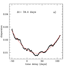
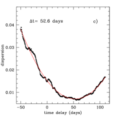
Figure 3: a) The dispersion function obtained when the normalisation of the light curves is determined directly from the data. Several local minima appear. A polynomial fit to the dispersion function (solid line) allows the determination of a time delay of $\Delta t\sim 34.4$ days. b) The corresponding result of the Monte-Carlo simulation for 100’000 slightly modified light curves: $\Delta t\sim 34.4\pm 1.4$ days. c) The dispersion function obtained for the light curves optimally shifted in magnitude (see text and Fig. 4). The function is now much smoother and has only one clear minimum at $\Delta t\sim 52.6$ days. d) The corresponding Monte-Carlo simulation result and the final time delay estimate: $\Delta t\sim 52.3\pm 1.6$ days.

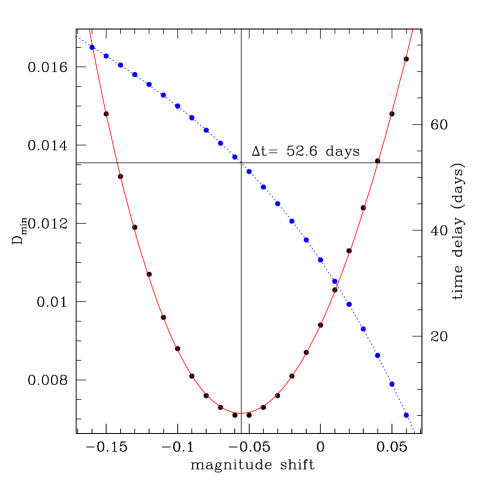
Figure 4: Value of the minimum D_min of the dispersion function, as a function of the magnitude shift between the two light curves. A fit (solid line) to the measurements yields the optimal magnitude shift $\Delta m=-0.056$. In the figure, a shift of 0 corresponds to the normalisation carried out directly on the data. The dotted line and the vertical axis on the right give the corresponding value of the time delay $\Delta t\simeq 52.6$ days (for one single realisation of the Monte-Carlo simulation).

A rough guess of the light curves shift indicates a time delay of about 50 days, i.e., 20 days longer than predicted in the discovery article (Morgan et al. Morgan03 (2003)). The brightest quasar image is the leading image, consistent with the arrival time surfaces presented in Saha et al. (Saha06 (2006)). Deriving a precise value for the time delay requires numerical methods. We use two very different techniques: the minimum dispersion method (Pelt et al. Pelt96 (1996)), and a polynomial fit to the data, e.g., as implemented in Kochanek et al. (Kochanek06a (2006)).

Our full dataset consists of 62 observing epochs. However, the photometric points for 5 of the epochs, marked by triangles in Fig. 2, deviate very far away from the general trend in the light curve of the quasar image B. These deviating points do not seem to be artifacts due to bad PSF or problems in the flux calibration. However, they introduce instable behaviour of the dispersion function and they do not reflect the otherwise smooth variation of the quasar. We choose to remove them from the data, prior to the time delay measurement.

4.1 The minimum dispersion method

The minimum dispersion method has been already applied many times to sparsely sampled light curves of lensed quasars (e.g., Pelt et al. Pelt98 (1998)). In this method, a guessed value is chosen for the time delay. The light curve of one quasar image is taken as a reference and the other is shifted by all the time delays to be tested in an arbitrarily long interval around the guess value. Pairs of points are formed with each point of the reference curve and its nearest corresponding neighbour in the shifted version of the second light curve, and a mean distance, in magnitude, is computed between the two curves. The best value of the time delay is the one that minimises the dispersion function constructed in that way. The method has to be used with caution, in particular when dealing with the flux normalisation of the light curves.

The mean magnitude of the data points of both light curves must be set to zero prior to their cross-correlation. However, the required normalisation factors are often determined from the light curves themselves, which can lead to a wrong normalisation as soon as the time delay becomes significantly long compared with the total length of the observations. Ideally, the normalisation must be done on the exact same portion of the intrinsic light curve of the quasar. In lensed quasars, we see several versions of this intrinsic light curve, which are shifted in magnitude and time, and clipped by the visibility window. Determining the factors directly from the data will therefore lead to a wrong normalisation.

If we normalise the data of SDSS J1650+4251 without taking into account the clipping of the light curves, the dispersion function, as shown in the upper left panel of Fig. 3, reaches its minimum for a $\Delta t=34.4$ days, with a secondary minimum around 55 days.

In order to estimate the correct normalisation factors, we follow an iterative procedure. We first estimate a rough normalisation factor from the data and we measure the minimum D_min of the dispersion function as well as the position $\Delta t$ of this minimum. We then slightly change the magnitude shift $\Delta m$ between the two light curves and we repeat the (D_min, $\Delta t$) measurement, so that we can explore the $\Delta m$ vs. D_min plane. The result is shown in Fig. 4. We consider that the correct magnitude shift between the light curves, and hence, the best time delay, is the one that minimises D_min. We obtain in that way $\Delta t=52.6$ days. Note that the magnitude shift that minimises D_min also gives a much cleaner, single-peaked dispersion function, as shown in the lower left panel of Fig. 3.

The accuracy on the time delay value is estimated using a statistical Monte-Carlo method: the data points in the light curves are slightly modified following a random Gaussian distribution that mimics the measured photometric errors, and the algorithm is run on these new modified data. The operation is repeated 100’000 times. The final time delay is the mean of the 100’000 measurements and the 1$\sigma$ error on this value is the error on this mean value. The result of the Monte-Carlo runs is shown in the right panels in Fig. 3. Our final value of the time delay using 57 epochs and the minimum dispersion method is $\Delta t=52.3\pm 1.6$ days.

Finally, note that these values do not take microlensing into account. The minimum dispersion method is, however, not very sensitive to low amplitude microlensing variations, as shown in Eigenbrod et al. (Eigenbrod05 (2005)). Adding microlensing does not change the time delay obtained above, but only slightly enlarges the distribution.

4.2 Polynomial fit to the light curves

A completely different approach to measure the time delay is to fit fully analytical functions to the light curves. An implementation of this type of method has been used in Kochanek et al. (Kochanek06a (2006)) and in Morgan et al. (Morgan06 (2006)), where Legendre polynomials were simultaneously fitted to the light curves of each quasar image. The time delay between each pair of images is one of the parameters of the fit, as well as the flux ratio of the images, corrected by the time delay. Our own implementation of the method does not use any stabilisation or smoothing term, which is not mandatory as long as the polynomial order is chosen in adequation with the number of data points in the light curves. In addition, a slow photometric variation is added to each light curve, in order to take microlensing into account.

This method is applied to the data in two ways, which are fully equivalent for a double quasar with little contribution of microlensing. First, we assume that the intrinsic photometric variation of the quasar is well represented by the light curve of the brightest quasar image A. The resulting microlensing contribution to the total variation in the light curve of the quasar image B then only reflects differential microlensing relative to the component A. A second way to implement the method, is to use one single light curve to represent the intrinsic variations of the quasar and to fit it simultaneously to the two quasar images. Two independent microlensing curves are fitted to the two light curves, allowing us to recover absolute microlensing curves. The fit to the data is performed in an iterative way and the algorithm is run 100’000 times on modified versions of the light curves following the statistical 1$\sigma$ errors on the photometry. As for the minimum dispersion method, the mean of the time delay distribution obtained in that way is taken as the time delay measurement, and its standard deviation as the 1$\sigma$ error (Fig. 5).

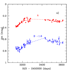
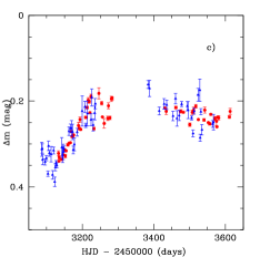
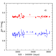
Figure 5: a) Best polynomial fit to the light curves. The order of the Legendre polynomial is 5 for the first season and 4 for the second season. b) Result of the Monte-carlo simulation for 100’000 modified light curves, leading to a mean time delay of $\Delta t=46.7\pm 2.2$ days. c) Light curves shifted by the time delay and corrected for slow microlensing variations. d) Microlensing variations of quasar image B relative to quasar image A, taken as a slow linear trend over the whole period of observation.

A critical step in the use of this fitting method is the choice of an optimal order for the Legendre polynomials. The data consist in two observing seasons, for which peak-to-peak variations and lengths are different. We therefore fit polynomials with different orders for the two seasons. We progressively increase the degree of the polynomial until the $\chi^{2}$ to the fit does not significantly improve. Microlensing is estimated in the same way, but we assume that the microlensing variations are slow compared to the intrinsic variations of the quasar. We therefore fit a single polynomial for both seasons. Fast microlensing, acting on time-scales of a week, is seen as an additional source of noise, and not as a systematic effect. Although we increase the degrees of the intrinsic and microlensing variations separately when trying different fits, both contributions are simultaneously fitted to the data, once the orders of the polynomial are chosen. The optimal combination of polynomial orders is N=5 for the first season of observation and N=4 for the second season. The microlensing variations are modeled using a simple linear slope. The difference between the fit and the data is shown in the lower right panel of Fig. 5, where the dispersion between the points is well compatible with the error bar on the individual points.

The two ways of applying the fitting method to the data are fully equivalent in the particular case of SDSS J1650+4251, as we only use a first order polynomial to model the microlensing and as there are only two light curves available. The time delays obtained in the two ways are indeed in agreement and yield $\Delta t=46.7\pm 2.2$ days. We find that slow microlensing is almost negligible in SDSS J1650+4251, with a global variation of 0.02 magnitude over 500 days (see Fig. 5). Taking the mean of the two values obtained using the minimum dispersion method and using the analytical fitting gives $\Delta t=49.5\pm 1.9$ days, which we take as our final estimate of the time delay. This translates into a relative error of 3.8 %, which is also in agreement with the predicted error bar from Eigenbrod et al. (Eigenbrod05 (2005)) for light curves with the same characteristics as the ones of SDSS J1650+4251. Finally, the $R$-band flux ratio between the quasar images, corrected for the time delay and the slow microlensing is $F_{\rm A}/F_{\rm B}=$ 6.2. Note that this flux ratio is constant in the time delay range.

5 Parametric modeling

The observational constraints available so far to model the potential well in SDSS J1650+4251 consist of the relative astrometry of the lensed images A and B with respect to the lensing galaxy G (Morgan et al. Morgan03 (2003)), and the image flux ratio measured in Section 4. Lacking a direct spectrum of the lensing galaxy, we assume a lens redshift $z_{\rm lens}$ = 0.58, as deduced from the MgII and FeII absorption lines observed in the spectra of the lensed quasar (Morgan et al. Morgan03 (2003)). This value of the lens redshift drives all the following estimates of the Hubble constant, which scales as (1+$z_{\rm lens}$).

Using the lensmodel package (v 1.08; Keeton KEE01 (2001)), we fit the lens system with (i) a Singular Isothermal Sphere model plus external shear (SIS) and (ii) a de Vaucouleurs model (DV). Due to the misalignment between components A, B and G of the lens system, we break the circular symmetry of the lens potential by adding external shear to the models. While it is likely that the gravitational potential of the lensing galaxy is not circular, the present observational data available for SDSS J1650+4251  do not offer enough constraints to allow the simultaneous fit of an elliptical potential plus external shear $\gamma$. However, the time delay of doubly imaged quasars where the lens lies almost on the line joining the two quasar images depends little on the structure of the quadrupole term of the potential (Kochanek KOC02 (2002)).

The constraints on our models are the relative astrometry of the lensed images with respect to the lensing galaxy (using a 1$\sigma$ error bar of 0.002″ on the positions of A and B and 0.03″ for G) and the flux ratio between A and B as found after correction from time delay and observed relative microlensing (i.e. $F_{\rm A}/F_{\rm B}=$ 6.2; Sect. 4). We consider a 5 % uncertainty on the flux ratio in order to include differential dust extinction due to the lensing galaxy, as suggested by the multi-color data of Morgan et al. (Morgan03 (2003)). The modification of the flux ratio due to the time delay uncertainty or microlensing is negligible over the period of observation, as pointed out in Section 4. In addition, our flux ratio does not differ much from that of Morgan et al. (Morgan03 (2003)), obtained 13 months before the start of our observations, but uncorrected for the time delay.

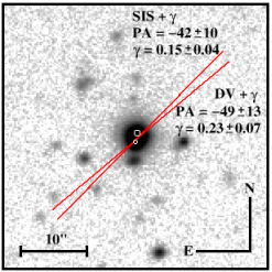
Figure 6: A zoom on the $R$-band image of SDSS J1650+4251 obtained at Maidanak Observatory (see Fig. 1). The positions of the quasar images are marked by white circles. The direction of the shear for our SIS+$\gamma$ and for the DV model is indicated by two lines. It does not point towards any specific galaxy in the field of view. Its large amplitude makes it mandatory to model the overall lensing potential.

The SIS+$\gamma$ model has just enough parameters to be exactly constrained by the data (i.e. zero degree of freedom), but the DV model has one more parameter, the effective radius $R_{e}$ of the lensing galaxy, that is unknown with the existing imaging data of SDSS J1650+4251. We therefore run our models with a fixed effective radius. We consider a wide range of plausible effective radii, $0.2$ kpc $<R_{e}<20$ kpc, and take the two boundaries for our calculations. These values enclose the range of measured effective radii in the Sloan-Lens ACS Survey (SLACS) sample of 15 early-type lens galaxies (Treu et al. TRE06 (2006)). They correspond to angular scales of $\theta_{e}\sim$ 0.3″ and 3.0″ at the lens redshift, adopting H₀  = 70 km s^-1 Mpc^-1, $\Omega_{\rm{m}}$ = 0.3, $\Omega_{\rm{\Lambda}}$ = 0.7.

Using the time delay measured in Section 4, $\Delta t=49.5\pm 1.9$ days, we find H₀ = 51.7${}^{+4.0}_{-3.0}$ km s^-1 Mpc^-1 with the SIS+$\gamma$ model. The DV+$\gamma$ model, with the lower bound value of $\theta_{e}=0.3$″, yields H₀  = 80.8 ${}^{+7.0}_{-3.0}$ km s^-1 Mpc^-1. Using the upper value $\theta_{e}=3.0$″, the DV model gives H₀ = 55.1${}^{+5.1}_{-3.8}$ km s^-1 Mpc^-1. Clearly only large values of the effective radius $\theta_{e}$ (ie $\theta_{e}>3^{\prime\prime}$) reconcile the value of H₀ given by the SIS+$\gamma$ and by the deVaucouleurs models. On the other hand, H₀= 72 km s^-1 Mpc^-1 is found for $\theta_{e}=$ 0.8″.

As previously argued, the unkown lens ellipticity is not a major source of uncertainty on the predicted value of H₀. In order to probe its effect, we fitted on the observed astrometry and flux ratio, 16200 elliptical lens models with fixed ellipticity $e$, lens major axis position angle $\phi$ and shear position angle $\theta_{\gamma}$, uniformly distributed in the ranges [0:0.4] ($e$) and [-90°:90°] ($\phi$ and $\theta_{\gamma}$). Following this procedure, we find that including the ellipticity in the lens model does not enlarge the distribution of predicted values of H₀.

All the 1$\sigma$ uncertainties quoted above are deduced by evaluating H₀ from 1$\sigma$ $\Delta\chi^{2}$ contours in the plane $\gamma$-$\theta_{\gamma}$ (i.e. $\Delta\chi^{2}=2.3$ for two degrees of freedom). The external shear predicted by both the SIS+$\gamma$ and DV models is large: $\gamma_{\rm SIS}=0.15\pm 0.04$ ($\theta_{\gamma}=-42^{\circ}\pm 10$) and $\gamma_{\rm DV}=0.23\pm 0.07$ ($\theta_{\gamma}=-49^{\circ}\pm 13$), for $\theta_{e}=0.3$″. The direction of the shear does not point towards obvious specific external perturber in Fig. 6. Its large amplitude suggests, however, that other mass clumps along the line of sight do modify the overall potential well.

6 Conclusions

The main result of the present work is the first time delay measurement of the COSMOGRAIL project, for the doubly imaged quasar SDSS J1650+4251. Our best estimate of the time delay is $\Delta t=49.5\pm 1.9$ days (1$\sigma$). This corresponds to a relative accuracy of 3.8 %. The $R$-band flux ratio of the two quasar images, corrected for microlensing and for the time delay, is $F_{\rm A}/F_{\rm B}=6.2\pm 5\%$.

The amplitude of the external shear in the circular lens models is larger than $\gamma=0.15$, and suggests that both external shear and ellipticity in the main lensing galaxy are necessary to model the total potential well. However, the present observational constraints available for SDSS J1650+4251  prevent us from introducing a lens ellipticity and position angle in the models. Deep, high resolution images of SDSS J1650+4251 will be necessary to estimate the latter two parameters.

With the present 3.8 % accuracy on the time delay, we can efficiently discriminate between families of lens models or, conversely, estimate H₀ assuming a lens model. Our results suggest that SIS models are not acceptable in order to match the current favored value of the Hubble constant (H₀  = 72 $\pm$ 8 km s^-1 Mpc^-1) and that only models of the lensing galaxy that have a de Vaucouleurs mass profile can reproduce it.

Slow microlensing is negligible in the first two seasons of monitoring, with a global variation of less than 0.02 mag over 500 days.

Finally, note that the redshift of the lensing galaxy is based on MgII and FeII absorption lines in the spectrum of the quasar images. Although the impact parameter necessary to form these lines is small, we cannot exclude that the true lens redshift does not correspond to the absorption lines, as in other systems (HE 1104-1805; Lidman et al. lidman2000 (2000)). A genuine spectrum of the lensing galaxy must be obtained to confirm its redshift.

Table 1: Photometry of SDSS J1650+4251 and of reference star #5, as in Fig. 2. The Julian date corresponds to HJD-2450000 days. The five points marked by an asterisk are not used in the determination of the time delay.

HJD	seeing [”]	mag A	$\sigma_{A}$	mag B	$\sigma_{B}$	mag star #5	$\sigma_{star\#5}$
3133.412	1.5	0.273	0.006	2.244	0.016	-0.175	0.013
3134.362	1.1	0.291	0.002	2.241	0.011	-0.166	0.004
3135.385	0.9	0.282	0.004	2.268	0.012	-0.177	0.008
3142.386	1.3	0.287	0.002	2.273	0.007	-0.167	0.003
3146.415	1.2	0.276	0.001	2.264	0.006	-0.178	0.002
3150.406	0.9	0.264	0.001	2.300	0.006	-0.176	0.001
3152.367	1.0	0.279	0.004	2.231	0.011	-0.172	0.008
3154.407	0.9	0.267	0.002	2.252	0.007	-0.175	0.003
3159.364	1.1	0.253	0.003	2.254	0.018	-0.174	0.005
3163.315	1.7	0.249	0.002	2.301	0.010	-0.173	0.003
3166.425	1.0	0.248	0.002	2.244	0.008	-0.177	0.003
3169.393	1.1	0.222	0.003	2.317	0.011	-0.189	0.006
3171.430	1.5	0.234	0.002	2.284	0.008	-0.172	0.004
3173.298	1.1	0.233	0.001	2.275	0.006	-0.168	0.002
3175.300	1.1	0.230	0.001	2.279	0.006	-0.178	0.001
3189.265	1.1	0.208	0.007	2.236	0.023	-0.172	0.012
3191.360	1.1	0.215	0.003	2.255	0.018	-0.167	0.004
3193.304	1.3	0.194	0.006	2.246	0.018	-0.166	0.012
3195.252	1.0	0.217	0.002	2.239	0.007	-0.170	0.004
3203.314*	1.4	0.186	0.001	2.345	0.007	-0.173	0.002
3209.256	1.0	0.189	0.003	2.198	0.010	-0.167	0.007
3213.256	1.0	0.166	0.003	2.190	0.010	-0.183	0.007
3216.310	1.7	0.149	0.006	2.189	0.018	-0.163	0.011
3219.281	1.6	0.151	0.004	2.198	0.018	-0.155	0.008
3221.234	1.0	0.178	0.002	2.241	0.009	-0.179	0.003
3224.209	1.2	0.140	0.005	2.228	0.015	-0.166	0.010
3232.187	1.1	0.215	0.003	2.198	0.009	-0.168	0.005
3246.163	1.3	0.133	0.013	2.148	0.035	-0.142	0.026
3248.138*	1.5	0.172	0.004	2.054	0.013	-0.114	0.007
3254.125	0.9	0.156	0.004	2.139	0.013	-0.160	0.007
3256.135	1.0	0.188	0.001	2.181	0.005	-0.173	0.003
3261.115	1.5	0.203	0.011	2.153	0.029	-0.178	0.017
3271.109	1.3	0.191	0.005	2.167	0.014	-0.183	0.009
3273.103	1.2	0.163	0.007	2.117	0.020	-0.176	0.013
3277.104	1.0	0.190	0.004	2.179	0.014	-0.191	0.007
3281.106	1.4	0.146	0.006	2.151	0.016	-0.167	0.011
3283.100	1.2	0.146	0.004	2.129	0.012	-0.164	0.008
3430.540	0.9	0.167	0.002	2.078	0.009	-0.135	0.003
3434.546	0.8	0.175	0.007	2.088	0.019	-0.143	0.009
3461.499	0.9	0.166	0.003	2.138	0.009	-0.150	0.005
3475.491	0.9	0.175	0.004	2.120	0.012	-0.179	0.008
3482.443	1.1	0.177	0.002	2.124	0.011	-0.149	0.004
3500.415	1.3	0.206	0.004	2.147	0.011	-0.168	0.008
3507.348	1.0	0.177	0.005	2.106	0.012	-0.153	0.009
3508.403*	0.9	0.199	0.003	2.222	0.009	-0.171	0.006
3511.303	1.0	0.172	0.007	2.153	0.018	-0.151	0.012
3517.383	0.8	0.163	0.004	2.146	0.012	-0.168	0.007
3524.391	0.9	0.194	0.002	2.118	0.006	-0.183	0.003
3533.412*	1.6	0.193	0.002	2.002	0.007	-0.171	0.004
3540.345	1.0	0.194	0.003	2.124	0.011	-0.168	0.006
3542.323	1.1	0.172	0.007	2.132	0.020	-0.194	0.014
3552.291	0.9	0.201	0.001	2.149	0.005	-0.179	0.001
3556.295	0.9	0.204	0.003	2.185	0.008	-0.176	0.005
3559.280	1.0	0.181	0.002	2.134	0.007	-0.160	0.004
3564.295*	1.3	0.228	0.001	2.300	0.007	-0.167	0.003
3570.247	1.0	0.192	0.005	2.094	0.015	-0.165	0.010
3575.323	1.3	0.198	0.010	2.084	0.026	-0.172	0.019
3576.264	1.0	0.211	0.001	2.195	0.008	-0.181	0.002
3578.275	1.2	0.189	0.002	2.133	0.007	-0.177	0.003
3581.284	1.2	0.190	0.005	2.176	0.012	-0.188	0.009
3611.225	1.2	0.188	0.003	2.161	0.008	-0.165	0.005
3613.201	1.5	0.175	0.007	2.156	0.018	-0.180	0.013