Antisymmetric Metric Field as Dark Matter

Abstract

We consider the generation and evolution of quantum fluctuations of a massive nonsymmetric gravitational field ($B$-field) from inflationary epoch to matter era in the simplest variant of the nonsymmetric theory of gravitation (NGT), which consists of a gauge kinetic term and a mass term. We observe that quite generically a nonsymmetric metric field with mass, $m_{B}\simeq 0.03(H_{I}/10^{13}~{}{\rm GeV})^{4}~{}{\rm eV}$, is a good dark matter candidate, where $H_{I}$ denotes the inflationary scale. The most prominent feature of this dark matter is a peak in power at a comoving momentum, $k\sim\sqrt{m_{B}H_{0}}/(1+z_{\rm eq})^{1/4}$, where $z_{\rm eq}$ is the redshift at equality. This scale corresponds roughly to the Earth-Sun distance.

I Introduction

Einstein’s theory of relativity has passed all experimental tests on laboratory and intermediate scales. On cosmological scales however, in order to get a successful description of the Universe’s dynamics one requires addition of dark matter and dark energy, both of unknown composition. An alternative is to extend Einstein’s theory and hope that a modified theory of gravitation would describe gravitation on cosmological scale without a need for dark matter and/or dark energy. Examples of extended theories of gravitation which have both been used as alternatives to dark matter Moffat (2005) are the nonsymmetric theory of gravitation (NGT) Moffat (1979) and MOND Milgrom (1983); Bekenstein (2004).

In Ref. Prokopec and Valkenburg (2006) we assumed that the antiymmetric tensor field $B$ is dynamical, and considered the cosmological evolution of quantum fluctuations generated in de Sitter inflation of a massless $B$-field, which is related by a duality transformation to the Kalb-Ramond axion field. We have further shown that the evolution of a massless $B$ field mimics that of a very light field. We then presented some early results on the evolution of a massive $B$-field, and observed that the scaling changes when the field becomes nonrelativistic in radiation era. From our analysis of quantum fluctuations of the physical mode of the antisymmetric field, which corresponds to the longitudinal ‘magnetic’ component, it follows that the field couples conformally during de Sitter inflation, such that the $B$-field correlator exhibits the spectrum of conformal vacuum fluctuations. This is contrary to what has been claimed based on studies of the Kalb-Ramond axion, which couples to gravitation just like a massless minimally coupled scalar field, and therefore exhibits a nearly scale invariant spectrum during inflation. In fact, because of the conformal coupling during inflation, there cannot be a physical observable which exhibits a scale invariant spectrum during inflation or subsequent epochs. There is amplification however, which is induced by the matching at the inflation-radiation transition, and based on which the spectral amplitude gets enhanced at superhorizon scales with respect to the conformal vacuum, but not enough to get a scale invariant observable. Finally we observed that the spectral features of the $B$ field fluctuations produced in inflation are similar to that of gravitational waves, making it thus an alternative probe of inflationary scale. There is an important difference in the spectrum between the primordial gravitons and the $B$ field fluctuations: while the primordial gravitons exhibit a scale invariant spectrum on superhubble scales, the $B$-field fluctuations are suppressed.

Building on an earlier work of Damour, Deser and McCarthy Damour et al. (1993) and Clayton Clayton (1996), Janssen and Prokopec Janssen and Prokopec (2006) have recently shown that there is no nonsymmetric geometric theory which yields a dynamical $B$ field and which is “problem free,” in the sense that the $B$-field dynamics is ghost free and it is not marred by instabilities. Furthermore the authors of Janssen and Prokopec (2006) have shown that the most general (problem free) quadratic action in the $B$ field is of the form,

$$S = S_{\rm HE}+S_{\rm B}\,,\qquad S_{\rm B}=\int d^{4}x{\cal L}_{\rm B}$$

$${\cal L}_{\rm B} = -\sqrt{-g}\frac{1}{12}H_{\mu\nu\rho}H^{\mu\nu\rho}-\sqrt{-g}\frac{1}{4}\Big{(}m_{B}^{2}+\xi{\cal R}\Big{)}B_{\mu\nu}B^{\mu\nu}\,,$$ (1)

where

$$H_{\mu\nu\rho}=\partial_{\mu}B_{\nu\rho}+\partial_{\nu}B_{\rho\mu}+\partial_{\rho}B_{\mu\nu}$$ (2)

is the antisymmetric field strength and

$$S_{\rm HE}=\int d^{4}x{\cal L}_{\rm HE}\,,\qquad{\cal L}_{\rm HE}=-\frac{1}{16\pi G_{N}}\Big{(}{\cal R}+2\Lambda\Big{)}$$ (3)

is the Hilbert-Einstein action, with $\Lambda$ being the cosmological constant. In this paper we work in the units in which, $1/(16\pi G_{N})=1$. From Eq. (1) we see that the coupling to the Ricci scalar ${\cal R}$ is the only allowed coupling to curvature.

In order to simplify the problem further, we drop the coupling to the Ricci scalar and set $\xi=0$ in Eq. (1). This term is expected to act as an additional mass term during inflation era and thus introduce additional breaking of conformal invariance. During radiation and matter era however, where the Ricci scalar is either zero (radiation era) or of the order of the Hubble parameter (matter era), we expect that the Ricci scalar term has no significant impact on the evolution of the $B$-field.

In a geometric theory the mass term is naturally induced by the cosmological constant, in which case Janssen and Prokopec (2006),

$$m_{B}^{2}\simeq 2\Lambda(1-2\rho+8\sigma)\,,$$ (4)

where $\rho$ and $\sigma$ are defined by the following decomposition of the metric tensor,

$$\bar{g}_{\mu\nu}=g_{\mu\nu}+B_{\mu\nu}+\rho B_{\mu}^{\;\alpha}B_{\;\alpha\nu}+\sigma B^{2}g_{\mu\nu}+{\cal O}(B_{\mu\nu}^{3})\,.$$ (5)

This is a general metric tensor decomposition in terms of the symmetric metric tensor ($g_{\mu\nu}$) and antisymmetric metric tensor ($B_{\mu\nu}$). Yet there is no reason to assume that the mass term is fully of geometric origin, and thus the relation (4) needs not to hold in general.

Equation (4) is also significant because it implies that, if the $B$ field is of a geometric origin, then it would be unnatural to assume that its mass vanishes. Indeed the current observations, based on the luminosity-redshift relation of distant supernovae Ia Perlmutter et al. (1999); Riess et al. (2004), suggest that the cosmological term today is of the order, $\Lambda\sim 10^{-84}~{}{\rm GeV}^{2}$. To maintain generality we assume in this work that the mass $m_{B}$ is unspecified and study its cosmological implications. In order to do that, we canonically quantise the massive $B$ field in inflation, and follow its subsequent dynamics in radiation and matter eras. Our main finding is that the $B$ field with a mass of the order,

$$m_{B}\simeq 0.03\Big{(}\frac{10^{13}~{}{\rm GeV}}{H_{I}}\Big{)}^{4}~{}{\rm eV}$$ (6)

which corresponds to a lengthscale, $m_{B}^{-1}\simeq 7\times 10^{-8}\big{(}{H_{I}}/{10^{13}~{}{\rm GeV}}\big{)}^{4}~{}{\rm m}$, is a good dark matter candidate.

Since the $B$ field is produced in inflation and does not couple to the matter fields, its spectrum is highly nonthermal. Indeed, we find that the spectral power is peaked at a comoving momentum, $k\simeq\sqrt{m_{B}H_{0}}/(1+z_{\rm eq})^{1/4}$, where $z_{\rm eq}$ is the redshift at matter-radiation equality, and corresponds to a physical scale at structure formation ($z\sim 10$), $k_{\rm phys}^{-1}\sim 2\times 10^{7}~{}{\rm km}$. This peak is generated as a consequence of a different nature of the vacuum states in inflation and radiation era. This is the main feature by which this dark matter can be distinguished from other dark matter candidates, which typically obey a thermal statistic.

Another important feature are Fourier space pressure oscillations, which occur after the second Hubble crossing. Although we find that the pressure of the $B$-field drops to zero before the decoupling of the cosmic photon fluid, the Fourier pressure components exhibit significant oscillations. These oscillations may have a potentially observable impact on the gravitational potentials, and they are thus the second distinct feature of our dark matter candidate. The physical significance of these spectral pressure oscillations should be further investigated.

II Stable linearised action

Taking the nonsymmetric gravity theory (NGT) as a starting point, one can perform an expansion of some general covariant geometrical action, in terms of antisymmetric perturbations on a symmetric background metric. The (linearised) action then reads Janssen and Prokopec (2006)

$$S_{\rm NGT}= \int d^{4}x\sqrt{-g}\left\{\overline{R}-2\Lambda-\tfrac{1}{12}F_{\mu\nu\rho}F^{\mu\nu\rho}\right.$$

$$\left.+\left(\tfrac{1}{4}m_{B}^{2}+\theta_{1}\overline{R}\right)B_{\mu\nu}B^{\mu\nu}+\theta_{2}\overline{R}_{\mu\alpha\nu\beta}B^{\mu\nu}B^{\alpha\beta}\right.$$

$$\left.+\theta_{3}B^{\alpha}\/_{\rho}B^{\rho\beta}\overline{R}_{\alpha\beta}+\mathcal{O}(B^{3})\right\},$$ (7)

where the parameters $\theta_{1},\theta_{2},\theta_{3}$ and $m_{B}$ are defined by the initial action. We choose to work up to second order in the nonsymmetric theory, and we will raise and lower indices with the symmetric background FLRW metric,

$$g_{\mu\nu}g^{\mu\rho}= \delta^{\rho}_{\nu},$$ (8)

$$g_{\mu\nu}B^{\mu\rho}= B_{\mu}\/^{\rho}.$$ (9)

In Ref. Damour et al. (1993), it was argued that NGT in general contains propagating ghosts or unacceptable constraints on dynamical degrees of freedom, when no cosmological term is present. For a simple choice of the action, $\theta_{n}=m_{B}=0$ ($n=1,2,3$), no ghosts are found in curved backgrounds Prokopec and Valkenburg (2006). Nevertheless, when considered in a FLRW or Schwarzschild background, the theory with $\theta_{1}\neq 0$ and/or $\theta_{2}\neq 0$ can develop instabilities even in the presence of a cosmological term Janssen and Prokopec (2006), putting into question the geometric origin of the antisymmetric tensor field. In the light of these results, we choose $\theta_{1}=\theta_{2}=0$. In addition for simplicity we choose $\theta_{3}=0$. The linearised action considered in this paper hence reads

$$S_{\rm HE}+S_{\rm B}= \int d^{4}x\sqrt{-g}\left\{\overline{R}-2\Lambda-\tfrac{1}{12}F_{\mu\nu\rho}F^{\mu\nu\rho}+\tfrac{1}{4}m_{B}^{2}B_{\mu\nu}B^{\mu\nu}\right\}.$$ (10)

In this equation we recognise the antisymmetric field strength of an antisymmetric 2-form, analogous to the Kalb-Ramond field Kalb and Ramond (1974),

$$F_{\mu\nu\rho} =\partial_{\mu}B_{\nu\rho}+\partial_{\nu}B_{\rho\mu}+\partial_{\rho}B_{\mu\nu}$$

$$=\overline{\nabla}_{\mu}B_{\nu\rho}+\overline{\nabla}_{\nu}B_{\rho\mu}+\overline{\nabla}_{\rho}B_{\mu\nu}.$$ (11)

II.1 Field equations

Following the action (10), the field equations for $B_{\mu\nu}$ read

$$a(\eta)^{2}\partial^{\rho}F_{\rho\mu\nu}-\frac{2a^{\prime}}{a}F_{0\mu\nu}+m_{B}^{2}a(\eta)^{2}B_{\mu\nu}= 0.$$ (12)

If we take the divergence of equation (12), multiplied with a factor of $a(\eta)^{-2}$, we are led to a self-consistency condition,

$$m_{B}^{2}\partial^{\mu}B_{\mu\nu}= 0.$$ (13)

Analogous to Maxwell theory, the antisymmetric tensor $B_{\mu\nu}$ can be decomposed in electric and magnetic components,

$$B_{0i}\quad=-B_{i0} =\quad E_{i}$$ (14)

$$B_{ij}\quad=-B_{ji} =\quad-\epsilon_{ijk}B_{k}.$$ (15)

In this decomposition the field equations become

$$E^{L}(x)= 0,$$ (16)

$$\left(\partial^{2}+m_{B}^{2}a(\eta)^{2}\right)\vec{E}^{T}(x)= 0,$$ (17)

$$\left(\partial^{2}-\frac{2a^{\prime}(\eta)}{a(\eta)}\partial_{0}+m_{B}^{2}a(\eta)^{2}\right)B^{L}(x)= 0,$$ (18)

$$\partial_{0}\vec{E^{T}}-\vec{\triangledown}\times\vec{B}^{T}(x)= 0.$$ (19)

Here we use superscripts ^T and ^L to denote the transverse and longitudinal parts of the vectors $\vec{E}$ and $\vec{B}$. Apparently the theory in this form possesses three degrees of freedom. However, if the mass term disappears, the field equations reduce to

$$\partial^{\rho}a(\eta)^{-2}F_{\rho\mu\nu}=0.$$ (20)

Equation (13) no longer results as a self-consistency condition. Though, the theory has gained a gauge freedom,

$$B_{\mu\nu} \rightarrow B^{\prime}_{\mu\nu}=B_{\mu\nu}+\partial_{\mu}\lambda-\partial_{\nu}\lambda,$$

$$F_{\mu\nu\rho} \rightarrow F^{\prime}_{\mu\nu\rho}=F_{\mu\nu\rho},$$

such that equation (13) may be imposed as a choice of gauge. Equation (20) is then by definition solved by

$$a(\eta)^{-2}F_{\rho\mu\nu}=\epsilon_{\rho\mu\nu\sigma}\partial^{\sigma}\phi.$$ (21)

Hence, the massless theory has only one (pseudoscalar) degree of freedom, which is known as the Kalb-Ramond axion. One could also have made an analysis of the degrees of freedom of this theory by the means of its dual action, which at linearised level reduces to a massive Abelian gauge field action, and therefore has three physical degrees of freedom Valkenburg (2006). However, in the presence of sources the dual theory contains nonlocal source terms, justifying the analysis in terms of the present variables. Note that the dual theory of the massive antisymmetric tensor field should not be mistaken for the massive Kalb-Ramond axion.

II.2 Power spectrum

What we eventually want to calculate is the spectrum of matter density fluctuations, $\mathcal{P}_{\delta\rho}(\vec{k},\eta)$, defined as $\rho^{-2}_{0}\left<\delta\rho(\vec{x},\eta)\delta\rho(\vec{x}^{\prime},\eta)\right>=\int\frac{dk}{k}\,\mathcal{P}_{\delta\rho}$. In this case $\mathcal{P}_{\delta\rho}=\frac{k^{3}}{2\pi^{2}}\left|\delta_{\vec{k}}\right|^{2}$, and $\delta_{\vec{k}}$ is the fourier transform of $\frac{\delta\rho}{\rho_{0}}$. $\rho_{0}$ denotes the average energy density and $\left<\cdot\right>$ denotes the averaging procedure. In the case of NGT, the power spectrum (i.e. the energy per decade in momentum space) is given by

$$\mathcal{P}_{\rm B}(\vec{k},\eta)=\frac{k^{3}}{2\pi^{2}}T_{0}\/^{0}(\vec{k},\eta),$$ (22)

where $T_{\mu\nu}$ is the stress-energy tensor of NGT,

$$T_{\mu\nu}=\frac{2}{\sqrt{-g}}\frac{\delta}{\delta g_{\mu\nu}}S_{\rm B}.$$ (23)

That is,

$$T_{0}\/^{0}(\vec{x},\eta)= \frac{1}{2a(\eta)^{6}}\left\{\left(\partial_{i}B_{j}(\eta,\vec{x})\right)^{2}+\left(\partial_{0}\vec{B}(\eta,\vec{x})+\nabla\times\vec{E}(\eta,\vec{x})\right)^{2}\right.$$

$$\left.\hskip 39.83368pt+a(\eta)^{2}m_{B}^{2}\left(\vec{E}(\eta,\vec{x})^{2}+\vec{B}(\eta,\vec{x})^{2}\right)\right\}.$$ (24)

III Canonical quantisation

Due to the antisymmetry we find that the $0i$-components of the canonical momenta are identically zero,

$$\Pi^{0i}=\frac{\sqrt{-g}}{4}F^{00i}=0.$$ (25)

This residual gauge freedom is fixed by adding the Fermi term Kalb and Ramond (1974),

$$\mathcal{L}\rightarrow\mathcal{L}+\frac{\lambda g_{\mu\nu}}{2}\left(\nabla_{\rho}B^{\rho\mu}\right)\nabla_{\sigma}B^{\sigma\nu},$$ (26)

such that the canonical commutation relations can still be imposed in a covariant way. The Fermi term does not affect the longitudinal magnetic component of the field.

In the next section we discuss the dynamics of the field during inflation, radiation and matter era. One result is that all momenta of interest, during inflation correspond to physical momenta which are highly relativistic. Effectively the theory during inflation is massless, hence the transverse degrees of freedom cannot obtain any energy. From the classical field equations for the transverse components, there is no indication that these degrees of freedom should become important at any time. In the following we will therefore neglect the transverse components.

In the context of quantising the theory with the Fermi term, it is then sufficient to say that the theory can be covariantly canonically quantised, and that for the component of interest we have the commutation relation

$$\left[\hat{\Pi}_{B_{L}}(x),\hat{B}_{L}(y)\right]=-\frac{i}{2}\delta^{4}(x-y).$$ (27)

Note that in Ref. Janssen and Prokopec (2006) it is shown that in fact the transverse degrees of freedom contain the instabilities of the geometrical theory, involving couplings to the curvature tensors in the action (7). Canonical quantisation of transverse degrees of freedom is carried out in Ref. Valkenburg (2006).

IV Inflation, radiation and matter era

We can perform a Fourier transformation,

$$B^{L}(x)= \int\frac{d^{3}k}{(2\pi)^{3/2}}\left\{e^{i\vec{k}\cdot\vec{x}}B^{L}\left(\eta,\vec{k}\right)a^{\phantom{{\dagger}}}_{\vec{k}}\right.$$

$$\left.+e^{-i\vec{k}\cdot\vec{x}}B^{L\ast}\left(\eta,\vec{k}\right)a_{\vec{k}}^{\dagger}\right\},$$ (28)

with the equal time relations

$$\left[a^{{\dagger}}_{\vec{k}},a^{\dagger}_{{\vec{k}}^{\prime}}\right]= 0,$$ (30)

$$\left[a^{\phantom{{\dagger}}}_{\vec{k}},a^{\phantom{{\dagger}}}_{{\vec{k}}^{\prime}}\right]= 0,$$ (31)

$$\left[a^{\phantom{{\dagger}}}_{\vec{k}},a^{\dagger}_{{\vec{k}}^{\prime}}\right]= \delta^{3}({\vec{k}}-{\vec{k}}^{\prime}).$$ (32)

The field equation for $B^{L}$ in momentum space becomes

$$\left(\partial_{0}^{2}+k^{2}-\frac{2a^{\prime}(\eta)}{a(\eta)}\partial_{0}+m_{B}^{2}a(\eta)^{2}\right)B^{L}(\eta,k)= 0,$$ (33)

Equations (30)–(32) are satisfied if the Wronskian satisfies

$$W[B^{L}(\eta,k),B^{\ast L}(\eta,k)]= ia(\eta)^{2},$$ (34)

We can conformally rescale $B^{L}$,

$$\tilde{B}^{L}=\frac{1}{a(\eta)}B^{L},$$ (35)

such that we have the field equation for $\tilde{B}^{L}$,

$$\left(\partial_{0}^{2}+k^{2}+m_{B}^{2}a(\eta)^{2}+\frac{a^{\prime\prime}(\eta)a(\eta)-2a^{\prime}(\eta)^{2}}{a(\eta)^{2}}\right)\tilde{B}^{L}= 0.$$ (36)

The expression for the power spectrum (22) containing only $B^{L}$ in momentum space becomes,

$$\mathcal{P}_{\rm B}=\frac{k^{3}}{4\pi^{2}a(\eta)^{4}} \left\{\left|\partial_{0}\tilde{B}^{L}(k,\eta)+\frac{a^{\prime}}{a}\tilde{B}^{L}(k,\eta)\right|^{2}+(k^{2}+a^{2}m_{B}^{2})\left|\tilde{B}^{L}(k,\eta)\right|^{2}\right\}.$$ (37)

IV.1 De Sitter inflation

Consider De Sitter inflation, in which the scale factor as a function of conformal time $\eta$ is given by

$$a(\eta)=\frac{-1}{H_{I}\eta}\quad\quad\mbox{(with $-\infty<\eta<\frac{-1}{H_{I}}$)},$$ (38)

with $H_{I}$ the Hubble constant during inflation. The field equation reads

$$\left(\partial_{0}^{2}+k^{2}+\frac{m_{B}^{2}}{H_{I}^{2}\eta^{2}}\right)\tilde{B}^{L}_{inf}(\eta,k)= 0,$$ (39)

solved by

$$\tilde{B}^{L}_{inf}(\eta,k)=\alpha_{B}^{inf}\sqrt{\eta}Z^{(1)}_{\frac{1}{2}\sqrt{1-(4m_{B}^{2}/H_{I}^{2})}}(k\eta)+\beta_{B}^{inf}\sqrt{\eta}Z^{(2)}_{\frac{1}{2}\sqrt{1-(4m_{B}^{2}/H_{I}^{2})}}(k\eta).$$ (40)

Here $Z^{(n)}_{\nu}$ denotes any general pair of Bessel functions Gradshteyn and Ryzhik (1994) that forms a basis for the solution space. For every momentum $k$ there has been an $\eta$ during inflation such that $k_{\rm phys}>m_{B}a(\eta)$. As during inflation the effectively massless $B^{L}$ field is conformally invariant, its vacuum state is given by the conformal vacuum Birrell and Davies (1982); Bunch and Davies (1978) at early time (as $\eta\rightarrow-\infty$). The vacuum state mode function reads,

$$\tilde{B}^{L}_{inf}(\eta,k) =-i\sqrt{\frac{\pi\eta}{4}}H^{(2)}_{\frac{1}{2}\sqrt{1-(4m_{B}^{2}/H_{I}^{2})}}(k\eta).$$ (41)

Note that in the limit when $m_{B}\rightarrow 0$, the field is in conformal vacuum. This is the relevant limit, since we are interested in the physical momenta which at the end of inflation satisfy the relation, $H_{I}\gg k/a(\eta_{end})\gg m_{B}$. Indeed, the physical momenta that are within the Hubble radius today (and of course smaller than the comoving $H_{I}$) all satisfy this condition. Moreover, since conformal invariance is broken by the stress energy tensor (24), from the point of view of energy density, superhorizon modes in fact undergo amplification during inflation. This is in agreement with the stress energy tensor of the massless Kalb-Ramond axion, which to a good approximation corresponds to the dual description during inflation.

IV.2 Radiation era

We choose the simple model of a sudden transition from inflation era to radiation era, with a scale factor

$$a(\eta)=H_{I}\eta\quad\quad\mbox{with $(\frac{1}{H_{I}}<\eta<\eta_{e})$}.$$ (42)

Conformal time at the time of radiation-matter equality is denoted by $\eta_{e}$.

The field equation for the longitudinal field in this era is given by

$$\left(\partial_{0}^{2}+k^{2}-\frac{2}{\eta}\partial_{0}+m_{B}^{2}H_{I}^{2}\eta^{2}\right)B^{L}_{\rm rad}(\eta,k)=0.$$ (43)

This field equation is in general solved by a special form of the confluent hypergeometric function, namely the Whittaker function $M_{\lambda,\mu}(x)$ Slater (1960). We prefer to choose a particular linear combination of Whittaker functions,

$$B^{L}_{\rm rad}(\eta,k)= \alpha_{B}^{\rm rad}(k)\tilde{M}^{(1)}\left[\frac{3}{4},\frac{k^{2}}{4m_{B}H_{I}};k\eta\right]+\beta_{B}^{\rm rad}(k)\tilde{M}^{(2)}\left[\frac{3}{4},\frac{k^{2}}{4m_{B}H_{I}};k\eta\right],$$ (44)

with

$$\tilde{M}^{(1)/(2)}\Big{[}\frac{3}{4},\zeta;k\eta\Big{]}= e^{\frac{i\pi}{4}}\sqrt{\frac{\pi H_{I}\eta}{4m_{B}}}\left[\frac{\zeta^{-\frac{3}{4}}}{\Gamma\left(\frac{5}{2}\right)}M_{i\zeta,\frac{3}{4}}\left(-i\frac{k^{2}\eta^{2}}{4\zeta}\right)\pm i\frac{\zeta^{\frac{3}{4}}}{\Gamma\left(-\frac{1}{2}\right)}M_{i\zeta,-\frac{3}{4}}\left(-i\frac{k^{2}\eta^{2}}{4\zeta}\right)\right],$$ (45)

because this tends to the asymptotic Bunch-Davies vacuum (i.e. the massless limit as $\eta\rightarrow 0$),

$$B^{L}_{\rm rad}(\eta,k)= \alpha_{B}^{\rm rad}(k)\eta^{\frac{3}{2}}H^{(1)}_{\frac{3}{2}}(k\eta)+\beta_{B}^{\rm rad}(k)\eta^{\frac{3}{2}}H^{(2)}_{\frac{3}{2}}(k\eta)$$

$$+\mathcal{O}\left(\frac{m_{B}^{2}}{H_{I}^{2}}\right).$$ (46)

The Hankel functions are given by

$$\eta^{\frac{3}{2}}H^{(1)}_{\frac{3}{2}}(k\eta) =\sqrt{\frac{2}{\pi k^{3}}}\left\{-i-k\eta\right\}e^{ik\eta},$$

$$\eta^{\frac{3}{2}}H^{(2)}_{\frac{3}{2}}(k\eta) =\sqrt{\frac{2}{\pi k^{3}}}\left\{i-k\eta\right\}e^{-ik\eta}.$$

With this choice of solution, the canonical condition, equation (34) is satisfied if

$$W[B^{L}_{\rm rad}(\eta,k),B^{L\ast}_{\rm rad}(\eta,k)]=\left(|\beta_{B}^{\rm rad}|^{2}-|\alpha_{B}^{\rm rad}|^{2}\right)ia(\eta)^{2}.$$ (47)

The coefficients $\alpha$ and $\beta$ in the solution are to be defined by a continuous matching of $B^{L}$ and its derivative at the time of transition from inflation to radiation era. For notational simplicity, we write $\tilde{M}^{(1)}$ and $\tilde{M}^{(2)}$ for the fundamental solutions in radiation era (44), and $\tilde{B}^{L}_{inf}$ for the mode function (41) during inflation all evaluated at the inflation-radiation transition. This then leads to

$$\alpha_{B}^{\rm rad} = \frac{1}{\tilde{M}^{(1)}{\tilde{M}^{(2)\prime}}-\tilde{M}^{(2)}{\tilde{M}^{(1)\prime}}}\left\{\tilde{B}^{L}_{inf}{\tilde{M}^{(2)\prime}}-\tilde{M}^{(2)}\tilde{B}^{L\,\prime}_{inf}\right\}$$ (48)

$$= \frac{1}{W\left[\tilde{M}^{(1)},\tilde{M}^{(2)}\right]}\left\{\tilde{B}^{L}_{inf}{\tilde{M}^{(2)\prime}}-\tilde{M}^{(2)}\tilde{B}^{L\,\prime}_{inf}\right\}$$

$$= -i\left\{\tilde{B}^{L}_{inf}{\tilde{M}^{(2)\prime}}-\tilde{M}^{(2)}\tilde{B}^{L\,\prime}_{inf}\right\}.$$

Likewise we find

$$\beta_{B}^{\rm rad}=i\left\{\tilde{B}^{L}_{inf}\tilde{M}^{(1)\prime}-\tilde{M}^{(1)}\tilde{B}^{L\,\prime}_{inf}\right\}.$$ (49)

Explicitly, that is

$$\alpha_{B}^{\rm rad} =-\frac{1}{2}\frac{H_{I}^{2}}{k^{2}}+\mathcal{O}\left(\frac{m_{B}}{H_{I}}\right)$$ (50)

$$\beta_{B}^{\rm rad} =-\frac{1}{2}\frac{H_{I}^{2}}{k^{2}}\left[1-2i\frac{k}{H_{I}}-2\frac{k^{2}}{H_{I}^{2}}\right]e^{2i\frac{k}{H_{I}}}+\mathcal{O}\left(\frac{m_{B}}{H_{I}}\right).$$ (51)

Thus we can see that for superhubble modes at the end of inflation,

$$\beta_{B}^{\rm rad}\simeq\alpha_{B}^{\rm rad}=-\frac{1}{2}\frac{H_{I}^{2}}{k^{2}}\Big{[}1+\mathcal{O}\left(\frac{m_{B}}{H_{I}},\frac{k}{H_{I}}\right)\Big{]}.$$ (52)

This Bogoliubov mixing Bogoliubov (1958); Birrell and Davies (1982) of the modes is caused by the mismatch of the vacua during inflation and radiation era, and loosely speaking can be thought of as particle production at the inflation-radiation transition.

IV.3 Matter era

During matter era the scale factor is given by

$$a(\eta)=\frac{H_{I}}{4\eta_{e}}(\eta+\eta_{e})^{2}.$$ (53)

The field equation for $\tilde{B}^{L}$ during matter era reads

$$\left(\partial_{0}^{2}+k^{2}-\frac{6}{\left(\eta+\eta_{e}\right)^{2}}+m_{B}^{2}\frac{H_{I}^{2}}{16\eta_{e}^{2}}(\eta+\eta_{e})^{4}\right)\tilde{B}^{L}_{\rm mat}(\eta,k)=0.$$ (54)

As the field equation contains a term $\propto\eta^{4}$, it cannot be solved analytically. However, for different values of $k\eta$ the field equation effectively takes various forms, shown in tabel 1.

Region	A Effective field equation		Scale
$\,I$	$\left(\partial_{X}^{2}+1-\frac{6}{X^{2}}\right)\tilde{B}^{L}_{\rm mat}(X)$	$=0\quad$	$\quad X^{2}\quad\ll$	$\frac{4k\eta_{e}}{\xi}$
$\,II$	$\left(\partial_{X}^{2}+1-\frac{6}{X^{2}}+\frac{\xi^{2}}{16k\eta_{e}}X^{4}\right)\tilde{B}^{L}_{\rm mat}(X)$	$=0\quad$	$\quad X^{2}\quad\simeq$	$\frac{4k\eta_{e}}{\xi}$
$\,III$	$\left(\partial_{X}^{2}+\frac{\xi^{2}}{16k^{2}\eta_{e}^{2}}X^{4}\right)\tilde{B}^{L}_{\rm mat}(X)$	$=0\quad$	$\quad X^{2}\quad\gg$	$\frac{4k\eta_{e}}{\xi}$  and   $X^{3}\gg\frac{4\sqrt{6}k\eta_{e}}{\xi}$

Table 1: The effective field equations for different values of $X\equiv k\tilde{\eta}\equiv k(\eta_{e}+\eta)$. The expressions are written in terms of the parameter $\xi\equiv\frac{m_{B}H_{I}}{k^{2}}$.

In region $I$ the solution is given by

$$\tilde{B}^{L}_{\rm mat}(\tilde{\eta},k)=\alpha_{B}^{\rm mat}\tilde{\eta}^{\frac{1}{2}}H_{\frac{5}{2}}^{(1)}(k\tilde{\eta})+\beta_{B}^{\rm mat}\tilde{\eta}^{\frac{1}{2}}H_{\frac{5}{2}}^{(2)}(k\tilde{\eta}),$$ (55)

with again the coefficients given by a continuous matching at the radiation-matter equality,

$$\alpha_{B}^{\rm mat}= \alpha_{B}^{\rm rad}\left(4i+\frac{2}{k\eta_{e}}-\frac{i}{2k^{2}\eta_{e}^{2}}\right)e^{-ik\eta_{e}}+\beta_{B}^{\rm rad}\frac{i}{2k^{2}\eta_{e}^{2}}e^{-3ik\eta_{e}},$$ (56)

$$\beta_{B}^{\rm mat}= \alpha_{B}^{\rm rad}\frac{-i}{2k^{2}\eta_{e}^{2}}e^{3ik\eta_{e}}+\beta_{B}^{\rm rad}\left(-4i+\frac{2}{k\eta_{e}}+\frac{i}{2k^{2}\eta_{e}^{2}}\right)e^{ik\eta_{e}}.$$ (57)

In region $II$ the solution of the field equation has to be solved numerically. In region $III$, the field equation reduces to

$$\left(\partial_{\tilde{\eta}}^{2}+\omega(\eta)^{2}\right)\tilde{B}^{L}_{\rm mat}(\tilde{\eta},k)=0.$$ (58)

If $\frac{\omega^{\prime}}{\omega}<\omega$ and $\frac{\omega^{\prime\prime}}{\omega}<\omega^{2}$, which is the case for the demanded values of $k\tilde{\eta}$ in this region, the solution can be approximated by

$$\tilde{B}^{L}_{\rm mat}(\tilde{\eta},k)=\frac{\alpha_{B}^{\rm mat}}{\sqrt{2\omega(\tilde{\eta})}}{\rm e}^{i\int^{\tilde{\eta}}d\eta\,\omega(\eta)}+\frac{\beta_{B}^{\rm mat}}{\sqrt{2\omega(\tilde{\eta})}}{\rm e}^{-i\int^{\tilde{\eta}}d\eta\,\omega(\eta)},$$ (59)

obeying the condition

$$W[u_{1},u_{1}^{*}]\simeq-i,\qquad u_{1}=\frac{1}{\sqrt{2\omega(\tilde{\eta})}}\,{\rm e}^{i\int^{\tilde{\eta}}d\eta\omega(\eta)}\,.$$ (60)

The explicit expressions for $\alpha$ and $\beta$ are rather complicated and for simplicity omitted.

V The spectrum

The power spectrum of the longitudinal mode, equation (37), in momentum space reads

$$\mathcal{P}_{\rm B}(\eta,k)= \frac{k^{3}}{4\pi^{2}a(\eta)^{4}}\left\{\left|\partial_{0}\tilde{B}^{L}(\eta,k)+\frac{a(\eta)^{\prime}}{a(\eta)}\tilde{B}^{L}(\eta,k)\right|^{2}\right.$$

$$\left.+(k^{2}+a(\eta)^{2}m_{B}^{2})\left|\tilde{B}^{L}(\eta,k)\right|^{2}\right\}.$$ (61)

In both radiation and matter era the subhubble spectrum grows as $\mathcal{P}_{\rm superH}(k)\propto k^{2}$, which is an infrared save spectrum. In the ultraviolet region the spectrum converges to the Bunch-Davies vacuum, $\mathcal{P}_{\rm subH}\propto\mbox{constant}$. In the intermediate region, the mass determines the height and blueness of the peak in the spectrum, hence in both radiation and matter era the mass term causes an enhanced spectrum with respect to the massless theory Prokopec and Valkenburg (2006). The evolution of one mode, fixed $k$, in both radiation and matter era is given in figures 1 and 2.

Figure 1: The evolution of a specific mode in momentum space, plotted for several values of $m_{B}H_{I}/k^{2}$. For low mass, a radiative spectrum is retrieved which redshifts $\propto a^{-4}$. The larger the mass, the earlier the evolution of a mode becomes massive as the mass exceeds the Hubble factor, where the redshift becomes $\propto a^{-3}\propto\eta\times a^{-4}$.

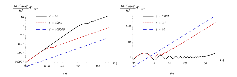
Figure 2: The evolution of a specific mode in momentum space during the matter era, plotted for several values of $m_{B}H_{I}/k^{2}$. For low mass, a radiative spectrum is retrieved which redshifts $\propto a^{-4}$. Again, the larger the mass, the earlier the evolution of a mode becomes massive, with a redshift of $\propto a^{-3}\propto\eta^{2}\times a^{-4}$.

Evolving in time, the damping of the modes in the density fluctuations evolves as $\mathcal{P}\propto a^{-2}$ on superhubble scales in both eras. For small enough mass, the spectrum remains relativistic in subhubble regions, that is, a damping of $\mathcal{P}\propto a^{-4}$. However, as soon the mass term $m_{B}^{2}a(\eta){{}^{2}}$ becomes dominant in the field equation, the evolution of a mode becomes non-relativistic, $\mathcal{P}\propto a^{-3}$, with a decaying oscillatory behaviour on top. A snapshot of the spectrum at fixed time $\eta$ is illustrated in figures 3 and 4.

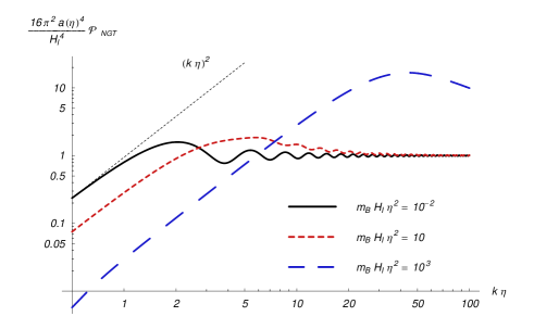
Figure 3: A snapshot of the spectrum during the radiation era at a fixed moment in time, plotted for several values of $m_{B}H\eta^{2}$. On superhubble scales the spectrum grows as $k^{2}$, whereas in the ultraviolet the spectrum becomes flat. Higher mass enhances the spectrum and blueshifts the peak, which lies at $k\simeq\sqrt{m_{B}H_{I}}$.

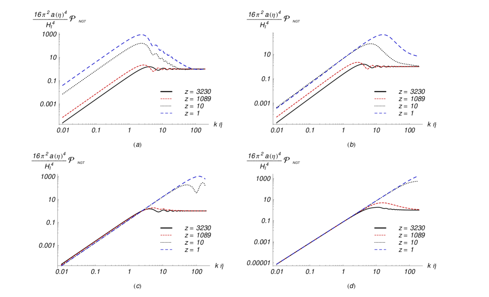
Figure 4: Snapshots of the spectrum during the matter era, plotted for several values of $\xi=m_{B}H\eta_{e}^{2}$. Figures (a)–(d) represent $m_{B}H\eta_{e}^{2}=10^{-6},10^{-2},1$ and $10$, respectively. The maximum value of the power spectrum still lies at $k\simeq\sqrt{m_{B}H_{I}}$.

It is the aforementioned non-relativistic evolution, depending on the scale factor, which makes the theory viable for providing the energy density of dark matter.

VI Energy density

As the mass term in the field equations grows with the scale factor, at a certain moment the energy density of the field switches from being dominated by relativistic modes to domination by non-relativistic modes, as previously explained.

When this switch in domination occurs, the energy density of the field grows with respect to the total energy density of the universe during the radiation dominated era.

If we assume that inflation can be described by a scalar inflationary model, such that

$$H_{I}^{2}=\frac{\rho_{\phi}}{3M_{P}^{2}},$$ (62)

where $M_{P}=(8\pi G_{N})^{-\frac{1}{2}}\simeq 2.4\times 10^{18}$ GeV is the reduced Planck mass, the energy density of the radiation field at the end of inflation equals

$$\rho_{\rm rad}(\eta_{end})=3H_{I}^{2}M_{P}^{2}.$$ (63)

The energy density of the nonsymmetric metric field is given by

$$\rho_{\rm B}(\eta)=\int\frac{dk}{k}{\cal P}_{B}(\eta,k).$$ (64)

In order to calculate the observable energy density, we subtract the conformal part of it, which effectively means that we impose an ultraviolet cut-off in the power spectrum. The excess energy-density comes from the modes which crossed the Hubble radius during inflation. The smallest of these momenta is given by the physical momentum at the beginning of inflation, $k_{phys}|_{in}\equiv k/a(\eta_{in})=H_{I}$, while the largest momentum is given by the physical momentum at the end of inflation, $k_{phys}|_{end}\equiv k/a(\eta_{end})=H_{I}$, where $\eta=\eta_{in}$ ($\eta=\eta_{end}$) denotes the conformal time at the beginning (end) of inflation. The latter momentum is also taken as the ultraviolet cut-off.

As the variable over which is integrated is $k\eta$, the minimum and maximum value of the domain of integration are given by $a_{in}a(\eta)$ and $a_{end}a_{\eta}$ respectively. Thus the energy density of the antisymmetric tensor field becomes

$$\rho_{\rm B}= \int_{a_{in}H_{I}}^{a_{end}H_{I}}\frac{dk}{k}\mathcal{P}_{\rm B}$$

$$= \frac{H_{I}^{4}}{4\pi^{2}a(\eta)^{4}}\left[-\frac{1}{4x^{2}}+\log x+\frac{\cos 2x}{4x^{2}}+\frac{\sin 2x}{2x}-{\rm ci}2x\right]_{a_{in}a(\eta)}^{a_{end}a(\eta)}.$$ (65)

where $x=k\eta$, $a_{in}=a(\eta_{in})$ and $a_{end}=a(\eta_{end})$. From equation (42) we have $a_{end}=1$, such that we may expand for small $a_{in}$,

$$\rho_{\rm B}= \frac{H_{I}^{4}}{4\pi^{2}a(\eta)^{4}}\left[\log a(\eta)-\frac{1}{2}+\log 2+\gamma_{E}+\frac{1}{2}a_{in}^{2}a(\eta)^{2}+\mathcal{O}\left(a(\eta)^{-2}\right)+\mathcal{O}\left(a_{in}^{3}\right)\right].$$ (66)

Here $\gamma_{E}$ denotes the Euler constant. Now we see that the energy density contains a subhubble term scaling as $a(\eta)^{-4}$, a term scaling as $a(\eta)^{-4}\log a(\eta)$ representing the continuous filling up of the density on horizon scales, and a small term $a_{in}a(\eta)^{-2}$ for the superhubble energy density. We assume the scale of inflation to be large enough to have $a_{in}a(\eta)<1$, such that the expansion is indeed allowed.

When the energy density is dominated by non-relativistic modes, the calculation of the energy density is less trivial. As the field is given in terms of $M_{\frac{ik^{2}}{4m_{B}H_{I}},\pm\frac{3}{4}}(-im_{B}H_{I}\eta^{2})$, the integral over all fourier modes too complicated to be evaluated exactly in an analytical fashion. However, we do know the asymptotic behaviour of the field in the infrared and the ultraviolet regions separately.

In the infrared the leading order of the spectrum is $\propto(k\eta)^{2}$. In the ultraviolet the spectrum becomes that of the massless theory.

This information together with a closer look at the field equation,

$$\left(\partial_{0}^{2}+k^{2}-\frac{2}{\eta^{2}}+m_{B}^{2}H_{I}^{2}\eta^{2}\right)\tilde{B}^{L}_{\rm rad}(\eta,k)=0.$$ (67)

allows a simple approximation. Note that during the radiation era the term $\propto\eta^{-2}$ represents $a(\eta)^{2}H(\eta)^{2}$, where $H(\eta)$ is the Hubble factor.

The approximation is the following: each of the second, third and fourth term in equation (67) has its own region in which it defines the behaviour of the field, but for each value of $k$ the mass eventually will dominate, leading to a scaling of $a(\eta)^{-3}$. Thus the energy density during the period of massive behaviour can be given in terms of the energy density during the period of massless behaviour.

The superhorizon modes all together are the first ones to start scaling as non-relativistic matter, as soon as the Hubble constant shrinks about below the mass, $m_{B}>\sqrt{2}H(\eta)$. That is the case when $a(\eta)\simeq\sqrt{H_{I}/m_{B}}$, such that

$$\mathcal{P}_{\rm superH}(k,\eta)\simeq\mathcal{P}^{\rm massless}_{\rm superH}(k,\eta)\rightarrow a(\eta)\sqrt{\frac{m_{B}}{H_{I}}}\mathcal{P}^{\rm massless}_{\rm superH}(k,\eta).$$ (68)

For sub-Hubble modes, the field starts scaling massive as soon as the wave vector shrinks below the mass, $m_{B}>k/a(\eta)$, when $a(\eta)\simeq k/m_{B}$, such that

$$\mathcal{P}_{\rm subH}(k,\eta)\simeq\mathcal{P}^{\rm massless}_{\rm subH}(k,\eta)\rightarrow\frac{m_{B}\,a(\eta)}{k}\mathcal{P}^{\rm massless}_{\rm subH}(k,\eta)$$ (69)

for $H(\eta)<\frac{k}{a(\eta)}<m_{B}$. The peak of the massive spectrum lies at the mode of which the physical momentum is equal to the mass when it crosses inside the Hubble radius, that is, $k^{2}=a(\eta)^{2}H(\eta)^{2}=a(\eta)^{2}m_{B}^{2}$,

$$k_{peak}= m_{B}\,a(\eta_{NR})$$

$$= \sqrt{H_{I}m_{B}},$$ (70)

where $\eta_{NR}$ denotes the moment in time of switching from relativistic to non-relativistic for the mode $k_{peak}$.

Now we can approximate the non-relativistic energy density by

$$\rho_{\rm B}= \int_{a_{in}H_{I}}^{\sqrt{m_{B}H_{I}}}\frac{dk}{k}a(\eta)\sqrt{\frac{m_{B}}{H_{I}}}\mathcal{P}^{\rm massless}_{\rm superH}(k,\eta)+\int_{\sqrt{m_{B}H_{I}}}^{m_{B}a(\eta)}{dk}\frac{m_{B}\,a(\eta)}{k^{2}}\mathcal{P}^{\rm massless}_{\rm subH}(k,\eta)$$

$$+\int_{m_{B}a(\eta)}^{a_{E}H_{I}}\frac{dk}{k}\mathcal{P}^{\rm massless}_{\rm subH}(k,\eta)$$

$$= \,\frac{H_{I}^{4}}{8\pi^{2}a(\eta)^{3}}\sqrt{\frac{m_{B}}{H_{I}}}\left[\mathcal{B}-2a(\eta)^{-1}\log\frac{m_{B}\,a(\eta)}{H_{I}}-2\sqrt{\frac{m_{B}}{H_{I}}}\right.$$

$$\left.+\mathcal{O}\left(a_{in}^{2}a(\eta)^{2},a(\eta)^{-2},(\sqrt{m_{B}H_{I}}\eta)^{-2}\right)\right].$$ (71)

In this expansion, $\mathcal{B}$ is the leading order coefficient, which can be determined by a numerical calculation of the energy density. In our approximation with a sudden relativistic-to-non-relativistic transition, we find $\mathcal{B}\simeq-2^{\frac{1}{4}}+2+2^{\frac{3}{4}}\log 2+2^{\frac{3}{4}}\gamma_{E}\simeq 1.35$. The third integral term only contributes if $m_{B}a(\eta)<H_{I}$. Of course, when $m_{B}a(\eta)>H_{I}$, the upper bound of the second integral becomes $a_{E}H_{I}$, and the logarithmic term in the energy density becomes nonexistent. This logarithmic term represents the contribution of superhubble but relativistic modes. This term damps quickly, and is neglected in the following. We assume that the scale of inflation is large enough to let $a_{in}a(\eta)\ll 1$ always, and we already made use of the fact that during the non-relativistic behaviour of the theory $\sqrt{m_{B}H_{I}}\eta>1$.

Taking account only for the leading order, we find for the NGT-to-radiation ratio when the field has become massive,

$$\frac{\rho_{\rm B}}{\rho_{\rm rad}}= \epsilon\,a(\eta)\sqrt{\frac{m_{B}}{H_{I}}}\qquad{\rm for\,\,}\epsilon=\frac{H_{I}^{2}\mathcal{B}}{3\pi m_{P}^{2}},$$ (72)

where $m_{P}^{2}=8\pi M_{P}^{2}$ is the unreduced Planck mass.

In order for the energy density to fully take account for the dark-matter energy density, it has to satisfy

$$\frac{\rho_{\rm B}}{\rho_{\rm rad}}=1\qquad\mbox{at $\eta=\eta_{e}$}.$$ (73)

Hence,

$$\epsilon\,{a_{\rm eq}}\sqrt{\frac{m_{B}}{H_{I}}}=1$$ (74)

This gives a rough approximation for the mass,

$$m_{B} =\frac{H_{I}}{\epsilon^{2}a_{\rm eq}^{2}}=\frac{H_{\rm eq}}{\epsilon^{2}}$$

$$=2.8\times 10^{-2}\left(\frac{10^{13}\,\mbox{GeV}}{H_{I}}\right)^{4}\,\mbox{eV}\,,$$ (75)

or

$$m_{B}^{-1} \simeq 7\times 10^{-8}\left(\frac{H_{I}}{10^{13}\,\mbox{GeV}}\right)^{4}\,\mbox{m}.$$ (76)

In the last line we used for the Hubble parameter at radiation-matter equality, $H_{\rm eq}=(z_{\rm eq}+1)^{3/2}H_{0}$, $H_{0}\simeq 1.4\times 10^{-42}\mbox{ GeV}$, $z_{\rm eq}=3230\pm 200$ and the scale factor $a_{\rm eq}/a_{0}=1/(z_{\rm eq}+1)$.

VII Pressure

Similar to the energy density, the pressure of the theory can be calculated as the pressure is given by the spatial components of the diagonal of the stress-energy tensor,

$$T_{i}\/^{i}=-3P.$$ (77)

If isotropy is assumed, that is $k_{i}k^{j}=\tfrac{1}{3}\delta_{i}\/^{j}\left|k\right|^{2}$ for $i=j$, the expression for the ’pressure per mode’ $P$ becomes,

$$P(\eta,k)= \frac{-1}{24\pi^{2}a(\eta)^{4}}\left[\left|\partial_{0}\tilde{B}^{L}(\eta,k)+\frac{a(\eta)^{\prime}}{a(\eta)}\tilde{B}^{L}(\eta,k)\right|^{2}\right.$$

$$\left.-3k^{2}\left|\tilde{B}^{L}(\eta,k)\right|^{2}-m_{B}^{2}a(\eta)^{2}\left|\tilde{B}^{L}(\eta,k)\right|^{2}\right].$$ (78)

The physical pressure can then be calculated by

$$P(\eta)=\int\frac{dk}{k}P(\eta,k).$$ (79)

When the field is dominated by relativistic modes, during radiation era this leads to,

$$P(\eta) =\frac{1}{4\pi^{2}a(\eta)^{4}}\left[\frac{1}{3}\log a(\eta)+\frac{1}{3}\log 2+\frac{1}{3}\gamma_{E}-\frac{1}{2}\right.$$

$$\left.-\frac{1}{6}a_{in}^{2}a(\eta)^{2}+\frac{\sin 2a(\eta)}{3a(\eta)}+\mathcal{O}\left(a_{in}^{4}a(\eta)^{4},a(\eta)^{-2}\right)\right].$$ (80)

Covariant conservation of the stress-energy tensor implies

$$\rho_{B}^{\prime}+3\frac{a(\eta)^{\prime}}{a(\eta)}\left(\rho_{B}+P\right)=0.$$ (81)

Comparing expressions (66) and (80), we find that energy conservation is indeed obeyed order by order in $\eta$.

On superhubble scales, $k\eta\ll 1$, the power spectrum and the pressure per mode are dominated by the first terms in relations (61) and (78). Thus one finds that for superhubble modes, both relativistic and non-relativistic, we have $P(\eta,k)\simeq-\tfrac{1}{3}\mathcal{P}_{\rm B}(\eta,k)$, in accordance with the scaling of $\rho\propto a(\eta)^{-2}$.

During inflation and during the matter era similar results are found for the relativistic modes, satisfying energy conservation.

This integration must be performed for the massive modes as well. However, for the same reasons as for the energy density, the pressure for the massive modes can only be either approximated or integrated numerically. We do not perform here a complete analysis of the pressure. Instead, we illustrate the pressure for one specific choice of parameters, and comment on how the pressure behaves for a general choice of parameters.

Figure 5: The ’pressure per mode’ for non-relativistic modes during radiation era, for $m_{B}H_{I}\eta^{2}=10^{3}$. Note that the x-axis is logarithmic, where the y-axis is linear. For superhubble scales the pressure scales as $-\tfrac{1}{3}\rho$, whereas on subhubble scales is averages aroung zero.

In figure 5 the ’pressure per mode’ is illustrated for a massive nonsymmetric field, with $m_{B}H_{I}\eta^{2}=10^{3}$. On superhubble scales, that is $k\eta\ll 1$, the pressure per mode behaves as mentioned above as $P(\eta,k)=-\tfrac{1}{3}\mathcal{P}_{\rm B}(\eta,k)$. On subhubble scales the pressure per mode becomes zero, conserving energy with a density scaling as $\rho\propto a(\eta)^{-3}$.

During inflation and matter era the behaviour of the pressure is consistent with covariant energy conservation as well. The result is that we have zero pressure at the time of decoupling when the field is massive. This is in agreement with the requirements on cold dark matter.

VIII Discussion and conclusions

We have considered the cosmology of a massive antisymmetric tensor field whose dynamics is given by the action (1). We follow the evolution of the vacuum fluctuations generated during an inflationary epoch, through inflation, radiation and matter era. We find that the antisymmetric field with a mass, $m_{B}=3\times 10^{-2}\left({10^{13}\,\mbox{GeV}}/{H_{I}}\right)^{4}\,\mbox{eV}$, results in the right energy density today to account for the dark matter of the Universe. This then implies that below the corresponding length scale, $m_{B}^{-1}\simeq 0.1\,\,{\rm\mu m}\left({H_{I}}/{10^{13}\,\mbox{GeV}}\right)^{4}$, the strength of the gravitational coupling may change, as it has been argued in Refs. Moffat and Sokolov (1996); Moffat (2005). This scale is about two orders of magnitude below the present experimental bound, which is of the order $10\mu\mbox{m}$ Will (2005). Note that the mass scale (75) depends strongly on the scale of inflation, such that, if the gravitational force law below the scale of $0.1\,\,{\rm\mu m}$ remains unchanged, would imply that, either the $B$ field is nondynamical, or the inflationary scale is lower than $10^{13}~{}{\rm GeV}$. Note that, in contrast to gravitons, the antisymmetric tensor field begins scaling as non-relativistic matter during radiation era, making it potentially the most sensitive probe of the inflationary scale.

The peak in the energy density power spectrum, generated as a consequence of a breakdown of conformal invariance in radiation era, corresponds to a comoving momentum scale of the order, $k\simeq\sqrt{m_{B}H_{0}}/(1+z_{\rm eq})^{1/4}$, where $z_{\rm eq}\simeq 3230$ is the redshift at matter-radiation equality. Hence the most prominent matter density perturbations at a redshift $z=10$, when structure formation begins, occur at a scale, $k_{\rm phys}^{-1}\sim 2\times 10^{7}\,{\rm km}$ (corresponding to a wavelength, $\lambda_{\rm phys}\sim 1\times 10^{8}~{}{\rm km}$, which is (co-)incidentally the Earth-Sun distance), which may boost early structure formation on these scales. We therefore expect that, when compared to other CDM models, this type of cold dark matter may induce an earlier structure formation. Even though the mass of the antisymmetric field is quite small (of the order of the heaviest neutrino mass, $m_{\nu}\sim 0.1\,\,{\rm eV}$), the antisymmetric tensor field dark matter is neither hot nor warm. Indeed, since the antisymmetric tensor field does not couple to matter fields, it cannot thermalise and its spectrum remains primordial, and thus highly non-thermal. Hence, in spite of its small mass the field pressure remains small, such that structure formation on small scales does not get washed out. Indeed, $P/\rho_{B}\simeq E_{kin}/(m_{B}c^{2})\sim 10^{-34}$ evaluated at ${k_{phys}=(k_{peak}/a)|_{today}}$, which is a tiny pressure.

Although the pressure converges to zero as the field becomes dominated by non-relativistic modes, the pressure per mode in Fourier space shows a characteristic oscillatory behaviour shown in figure 5. These oscillations may influence cosmological perturbations in a manner analogous to Sakharov oscillations Albrecht et al. (1994), which in turn may produce an observable imprint in the cosmic background photon fluid. This question deserves further investigation.

References

• Moffat (2005) J. W. Moffat, JCAP 0505, 003 (2005), eprint astro-ph/0412195.
• Moffat (1979) J. W. Moffat, Phys. Rev. D19, 3554 (1979).
• Milgrom (1983) M. Milgrom, Astrophys. J. 270, 365 (1983).
• Bekenstein (2004) J. D. Bekenstein, Phys. Rev. D70, 083509 (2004), eprint astro-ph/0403694.
• Prokopec and Valkenburg (2006) T. Prokopec and W. Valkenburg, Phys. Lett. B636, 1 (2006), eprint astro-ph/0503289.
• Damour et al. (1993) T. Damour, S. Deser, and J. G. McCarthy, Phys. Rev. D47, 1541 (1993), eprint gr-qc/9207003.
• Clayton (1996) M. A. Clayton, Class. Quant. Grav. 13, 2851 (1996), eprint gr-qc/9603062.
• Janssen and Prokopec (2006) T. Janssen and T. Prokopec (2006), eprint gr-qc/0604094.
• Perlmutter et al. (1999) S. Perlmutter et al. (Supernova Cosmology Project), Astrophys. J. 517, 565 (1999), eprint astro-ph/9812133.
• Riess et al. (2004) A. G. Riess et al. (Supernova Search Team), Astrophys. J. 607, 665 (2004), eprint astro-ph/0402512.
• Kalb and Ramond (1974) M. Kalb and P. Ramond, Phys. Rev. D9, 2273 (1974).
• Valkenburg (2006) W. Valkenburg, Linearised nonsymmetric metric perturbations in cosmology (2006), master’s thesis at the ITP of Utrecht University, available at http://www1.phys.uu.nl/wwwitf/Teaching/Thesis.htm.
• Gradshteyn and Ryzhik (1994) I. S. Gradshteyn and I. M. Ryzhik, Table of integrals, series and products (Academic Press, New York, USA, 1994), —c1994, 5th ed. completely reset, edited by Jeffrey, Alan.
• Birrell and Davies (1982) N. D. Birrell and P. C. W. Davies, QUANTUM FIELDS IN CURVED SPACE (Cambridge University Press, London, England, 1982), cambridge, Uk: Univ. Pr. ( 1982) 340p.
• Bunch and Davies (1978) T. S. Bunch and P. C. W. Davies, Proc. Roy. Soc. Lond. A360, 117 (1978).
• Slater (1960) L. J. Slater, Confluent Hypergeometric Functions (Cambridge University Press, London, England, 1960).
• Bogoliubov (1958) N. Bogoliubov, Sov. Phys. JETP 7, 51 (1958).
• Moffat and Sokolov (1996) J. W. Moffat and I. Y. Sokolov, Phys. Lett. B378, 59 (1996), eprint astro-ph/9509143.
• Will (2005) C. M. Will (2005), eprint gr-qc/0510072.
• Albrecht et al. (1994) A. Albrecht, P. Ferreira, M. Joyce, and T. Prokopec, Phys. Rev. D50, 4807 (1994), eprint astro-ph/9303001.