Confronting X-ray Emission Models with the Highest-Redshift Kiloparsec-scale Jets: the $z$=3.89 Jet in Quasar 1745+624

Abstract

A newly identified kiloparsec-scale X-ray jet in the high-redshift $z$=3.89 quasar 1745+624 is studied with multi-frequency Very Large Array, Hubble Space Telescope, and Chandra X-ray imaging data. This is only the third large-scale X-ray jet beyond $z>$ 3 known and is further distinguished as being the most luminous relativistic jet observed at any redshift, exceeding $10^{45}$ erg/s in both the radio and X-ray bands. Apart from the jet’s extreme redshift, luminosity, and high inferred equipartition magnetic field (in comparison to local analogues), its basic properties such as X-ray/radio morphology and radio polarization are similar to lower-redshift examples. Its resolved linear structure and the convex broad-band spectral energy distributions of three distinct knots are also a common feature among known powerful X-ray jets at lower-redshift. Relativistically beamed inverse Compton and ‘non-standard’ synchrotron models have been considered to account for such excess X-ray emission in other jets; both models are applicable to this high-redshift example but with differing requirements for the underlying jet physical properties, such as velocity, energetics, and electron acceleration processes. One potentially very important distinguishing characteristic between the two models is their strongly diverging predictions for the X-ray/radio emission with increasing redshift. This is considered, though with the limited sample of three $z>$ 3 jets it is apparent that future studies targeted at very high-redshift jets are required for further elucidation of this issue. Finally, from the broad-band jet emission we estimate the jet kinetic power to be no less than $10^{46}$ erg/s, which is about 10$\%$ of the Eddington luminosity corresponding to this galaxy’s central supermassive black hole mass ${\cal M}_{\rm BH}$ $\;\buildrel>\over{\sim}\;$$10^{9}\,{\cal M}_{\odot}$ estimated here via the virial relation. The optical luminosity of the quasar core is about ten times over Eddington, hence the inferred jet power seems to be much less than that available from mass accretion. The apparent super-Eddington accretion rate may however suggest contribution of the unresolved jet emission to the observed optical flux of the nucleus.

ApJ, accepted (12 Jun 2006)

1 Introduction

Figure 1: VLBI 2.3 GHz map of the parsec-scale jet in quasar 1745+624 from averaging 6 images from the USNO database (4 mas circular beam plotted on bottom left). The quasar core is the peak (239.0 mJy/bm) toward the upper left. The lowest contour level is 0.3 mJy/bm (2 times the measured rms in the image) increasing by factors of $\sqrt{2}$.

Figure 2: Multi-frequency VLA images of 1745+624. The $\sim$2.5^′′ long radio jet extending to the southwest of the core (placed at the origin) is seen clearly. The lowest contour levels are 0.60, 0.33, 0.40, and 0.45 mJy/beam (3 times the measured off source rms in the images), at 1.5, 4.9, 8.5, and 15 GHz, respectively. The positive levels (solid contours) are spaced by factors of $\sqrt{2}$ up to the image peaks of 484, 441, 464, and 577 mJy/beam. The elliptical restoring (naturally weighted) beams are plotted at the bottom left corner: their dimensions are 0.530^′′$\times$0.340^′′ at PA=–72^∘, 0.490^′′$\times$0.305^′′ at PA=–67^∘, 0.255^′′$\times$0.204^′′ at PA=–29^∘, and 0.182^′′$\times$0.128^′′ at PA=–74^∘.

Figure 3: VLA 4.9 GHz total intensity [I; left] and polarized intensity [P; right] images of 1745+624 at 0.35^′′ resolution (beam plotted in bottom left). Contour levels begin at 0.35 (I) and 0.16 (P) mJy/bm, and increase by factors of $\sqrt{2}$ up to peaks of 441.4 (I) and 18.1 (P) mJy/bm. The tick marks show the orientation of the electric vector position angles, with a correction of –6^∘ applied corresponding to the integrated rotation measure of 28.4$\pm$0.5 radians m^-2 (Oren & Wolfe, 1995). Selected fractional polarization levels are indicated.

Quasars form a class of objects that frequently warrant superlatives in their descriptions: 1745+624 (4C+62.29) is no exception. It was identified as one of the highest redshift X-ray quasars at the time of its discovery ($z$=3.87; Becker, Helfand, & White, 1992) from spectroscopic followup of statistically significant sources from the Einstein X-ray Observatory. Further optical spectroscopy by Stickel (1993) refined the redshift to $z$=3.89, affirmed by Hook et al. (1995); the latter value is adopted here. After the Einstein detection, it was established as a bona fide X-ray source by ROSAT (Fink & Briel, 1993), ASCA (Kubo et al., 1997), and BeppoSAX (Donato et al., 2005).

By virtue of its high-redshift, it is one of the most radio-luminous quasars known (cf. Figure 1 of Jester, 2003) – its observed 1.4 GHz luminosity, $L_{\rm 1.4GHz}=10^{29}$ W Hz^-1, is over an order of magnitude greater than that of the archetype luminous quasar 3C 273 (Conway et al., 1993). It is probably no coincidence that its 2.5^′′ long jet (18 kpc projected; Becker, Helfand, & White, 1992) is also the most luminous radio jet currently known (that we are aware of; cf. Liu & Zhang, 2002; Cheung et al., 2005b), accounting for $\sim$1/4th of the source’s total 1.4 GHz luminosity.

This quasar is of interest to us because of this prominent radio jet, visible on both milli-arcsecond (Taylor et al., 1994; Fey & Charlot, 2000, Figure 1) and arcsecond-scales (Figures 2 & 3). We were prompted to identify such high-redshift systems with large-scale jets after the Chandra X-ray Observatory detection of a $\sim$2.5^′′ long X-ray extension (Siemiginowska et al., 2003; Yuan et al., 2003; Cheung, 2004) in the $z$=4.3 quasar GB 1508+5714 (Hook et al., 1995). Subsequent VLBA imaging of GB 1508+5714 has revealed a parsec-scale jet that can be traced out to $\sim$100 milli-arcseconds (0.7 kpc projected; Cheung et al., 2006), aimed in the general direction of the kpc-scale structure, supporting the jet interpretation. These are the two most distant quasars with a kiloparsec-scale jet detected at any wavelength (Cheung et al., 2005b).

The identification of such systems in the early Universe is extremely interesting for a number of reasons. Jets are signposts for “active” black hole/accretion disk systems (e.g., Begelman, Blandford, & Rees, 1984), requiring central nuclei of high-$z$ galaxies to be sufficiently well-developed to sustain gravitational collapse. At such early epochs, it is remarkable that the jet production process is apparently efficient and persists long enough ($>$Myr) to have produced such large (10’s–100’s kpc-scale) structures. In this context, jets may even serve as tracers of the directionality of the BH/disk axis in these early accreting systems, as chronicled in the “bumps and wiggles” in our jet images. Also, these jets are an efficient means to shock heat ambient gas thus triggering early star formation (e.g., Rees, 1989).

Among other important issues, such high-redshift systems are potentially very important to our understanding of the emission processes responsible for the production of the broad-band jet emission, and the X-rays in particular. Although the number of quasars with kpc-scale jets detected in the X-rays is growing (Harris & Krawczynski, 2006), the origin of this radiation is still in active debate. Schwartz (2002) noted early on that a comparison of cosmologically distant jets with local examples could in principle provide crucial arguments to the debate. This is because the two main contending models for the X-ray emission of large-scale quasar jets – synchrotron radiation and inverse Compton scattering of the cosmic microwave background (IC/CMB) – have, in their simplest versions, markedly different predictions of the X-ray jet properties with redshift (see § 3.2.4).

A high-resolution Chandra image of the $z$=3.89 quasar 1745+624 was obtained in an early observing cycle (Table 1) and X-ray emission from the arcsecond-scale radio jet is in fact detected and is quite prominent also. Apart from the GB 1508+5714 case mentioned above, evidence has been presented recently for at least one more high-$z$ quasar with extended X-ray emission (J2219–2719 at $z$=3.63; Lopez et al., 2006) with a radio counterpart (Cheung et al., 2005b, and manuscript in preparation). This makes 1745+624 one of only three very high-redshift ($z>$3) systems with extended X-rays associated with a radio jet.

With the scarcity of such high-redshift systems and their importance in current discussions of X-ray jet emission models, we have independently analyzed the archival Chandra data. It was also realized that 1745+624 hosts an exceptional jet making it conducive to study. This is because while both the GB 1508+5714 and J2219–2719 cases each show a single faint ($\sim$1 mJy at 1.4 GHz) arcsecond-scale feature separated from their bright nuclei, the 1745+624 jet is 2 orders of magnitude brighter than the other two cases and shows resolved structure. In addition, it is the most luminous X-ray jet observed thus far (cf., Harris & Krawczynski, 2006).

To fully exploit the potential of the Chandra observation, we have also analyzed archival multi-frequency imaging data from the Very Large Array (VLA), and a Hubble Space Telescope (HST) image to map the spectral energy distributions of the extended components in the quasar jet. These data, along with a new deep very long baseline interferometry (VLBI) map of the extended subarcsecond-scale jet are described in §§ 2.1–2.4, with a critical assessment of the derived spectra of the kpc-scale components in § 2.5. The physical properties of these extended components are then discussed (§ 3), with comparisons made to the other two quasars with X-ray detected knots at comparably high-redshift ($z\lower 2.15277pt\hbox{$\;\buildrel>\over{\sim}\;$}$3). These distant examples are compared to other currently known X-ray jets in quasars at lower redshift ($z\lower 2.15277pt\hbox{$\;\buildrel<\over{\sim}\;$}$2) in light of expectations from synchrotron and inverse Compton emission models. Our results are summarized in § 4.

2 Multi-Telescope Archival Data and Analysis

2.1 Deep 2.3 GHz VLBI map of the Parsec-scale Jet

VLBI maps of 1745+624 show a prominent parsec-scale jet and the emission fading with distance out to $\sim$40 mas (Taylor et al., 1994; Fey & Charlot, 2000). The lower frequency, 2.3 GHz USNO Radio Reference Frame Image Database maps (RRFID, Fey & Charlot, 2000) suggest that the jet is even more extended. We therefore uniformly reprocessed the six best ($u,v$) datasets at this frequency from the RRFID (obtained between 1997 March to 1998 August) and produced images on the same grid, reconvolved with a common 4 mas beam. We then averaged the 6 images to suppress the noise in the background resulting in improved definition of the outer jet (Figure 1). The parsec-scale jet in this “average” image is now clear out to $\sim$110 mas (0.8 kpc projected) allowing us to trace (§ 3.1) the VLBI-scale emission to the outer structure sampled by the VLA data (Figure 2 and § 2.2).

At 4 mas resolution, the initial bright segment of the VLBI jet is oriented at position angle (PA) 212^∘ and contains two prominent peaks at roughly 14 mas (22.3 mJy/bm) and 23 mas (10.4 mJy/bm). At $\sim$50 mas from the core, the jet position angle increases (by $\sim$4^∘) and transitions to the outer fainter portion. Curiously, the eastern ridgeline of the outer portion lines up with the central PA of the inner jet. The integrated flux of the visible jet in the 2.3 GHz map is $\sim$110 mJy with the outer portion contributing about 20 mJy of this. We measure a jet to counter-jet ratio of $>$50 (defined as the ratio of the peak to 3 times the rms noise on the counter-jet side) of the first visible peak in the 2.3 GHz map.

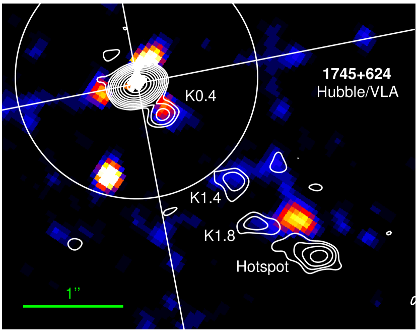
Figure 4: HST STIS (color) and VLA 14.9 GHz (contours; see Figure 2) images of the immediate field around quasar 1745+624. A model of the central optical source from fitting a series of elliptical isophotes has been subtracted, out to approximately 1.2^′′ (the radius of the pictured circle). The white lines crossing the nucleus indicate the directions of the main diffraction spikes in the image. The main knots in the jet discussed in the text are labeled.

2.2 Very Large Array

In light of the high signal-to-noise (S/N) ratio Chandra detection of the arcsecond-scale jet in 1745+624 (§ 2.4), we desired comparable information about its structure and spectra in the radio band.

Becker, Helfand, & White (1992) first discovered the extended radio emission in short VLA observations at 1.5, 5 and 15 GHz. The two main X-ray emitting knots which we dub K1.4 and K1.8 (indicating their distance from the core in arcseconds), and the terminal (brightest) jet feature at 2.5^′′ are readily identifiable in their 5 GHz map. For the sake of discussion, we classify the terminal knot, K2.5, as the radio “hot spot” in the context of similar X-ray detected features in other powerful jets (see below and § 3.3). Stickel (1993) noted also an 8.5 GHz VLA detection of this terminal feature by Patnaik et al. (1992) from a 100 sec. observation, though no image is presented. These four datasets form the basis of our radio analysis of the jet. At the two higher frequencies, these data are supplemented by the only other available VLA datasets – sparse snapshots from the more compact configurations to help fill in the shorter ($u,v$) spacings (see Table 1 for a summary of the data).

The data were obtained from the NRAO archive and calibrated in AIPS (Bridle & Greisen, 1994) utilizing scans of the calibrators 3C 48 and 3C 286 to set the amplitude scale. In the high-resolution A-configuration 15 GHz experiment (program AB414; Table 1), 3C 48 is heavily resolved so could not be relied on for this purpose. Fortunately, the phase calibrator 1803+784 was monitored frequently at this frequency by the UMRAO (Aller et al., 2003) and was found to be fairly stable over the two month period bracketing the VLA epoch (within $\sim$7$\%$ of the average of 3 Jy over 7 observations), so the amplitude scale was set with this data. The calibrated ($u,v$) data were exported into the Caltech DIFMAP package (Shepherd, Pearson, & Taylor, 1994) for self-calibration and imaging. The multi-frequency images were registered on the image peaks, i.e., the arcsecond-scale radio core. This registration must be good to within a small fraction of the VLA beams because the majority of the VLBI flux is concentrated within a few 10’s mas (§ 2.1).

Improving on the previous studies, we were able to separate and detect emission from the radio hot spot and the jet at all four frequencies (Figure 2). The 1.5 GHz image is a “super-resolved” image, created by reconvolving the data with a beam 1/3rd of the uniformly weighted one. An excess due to the jet is apparent (Figure 2). There is also an apparent excess adjacent to the core, on the side opposite of the visible jet; a similar excess is seen in the 5 GHz image. This could be suggestive of real emission on the counterjet side, although it is equally likely that they are spurious due to the gaps in ($u,v$) coverage of the datasets.

We considered the individual knot spectra (§ 2.5) but were concerned with the differing ($u,v$) coverages affecting the spectral measurements of the jet. To mitigate against this, we tapered and convolved the three higher-frequency images with a common 0.35^′′ beam (see e.g., Figures 3 & 5) and integrate the radio jet emission over several beamwidths when we measured the ”total” jet spectral index between the 3 frequencies (§ 2.5).

Additional polarization leakage-term calibration of the 5 GHz dataset was performed using observations of the calibrator, 1748–253, from an adjacent program AM337. The electric vector position angle (EVPA) of the resultant polarization image was determined by setting the EVPA of 3C 48 to 106^∘. The integrated rotation measure (RM) of 28.4$\pm$0.5 radians m^-2 (Oren & Wolfe, 1995) toward 1745+624 amounts to a small correction of –6^∘ at 5 GHz, and this correction has been applied to the polarization map in Figure 3.

At 5 GHz, the initial segment of the radio jet is highly polarized at $\sim$20$\%$ out to knot K1.4 with stronger interknot polarization of 30$\%$. The RM corrected map shows the EVPA perpendicular to the direction of the jet along most of this length, i.e., the implied magnetic field is parallel to the jet – quite typical in powerful one-sided jets (Bridle & Perley, 1984). Also typical is the low polarization in the core ($\sim$4$\%$).

The parallel-to-the-jet magnetic field configuration roughly continues into K1.8 and the terminal radio feature, which we classify as a hot spot based on its terminal position and compactness. The hot spot is unresolved with an average deconvolved major axis of 0.15^′′ and aspect ratio of 0.5 elongated at position angle of 254^∘ (fits consistent between the 5, 8.5, and 15 GHz datasets). This outer portion of the jet exhibits lower radio polarization levels of $\sim$5–6$\%$. The polarization pattern in K1.8 is not uniform and field cancellation may account for its low polarization.

The dimensions of the jet knots, K1.4 and K1.8, are not obviously resolved in our highest resolution (8.5 and 15 GHz) images though these are the frequencies at which the jet is faintest. We set an upper limit to their angular sizes (diameters) of 0.2^′′ based on these data.

Lastly, a new radio knot is found in the highest resolution (15 GHz) image 0.4^′′ from the nucleus (K0.4). Though not well-separated from the nucleus in the lower-resolution images, some excess emission presumably from K0.4 is seen connecting the core to the outer jet in all three lower-frequency maps (Figure 2). Its identification in the 15 GHz data helps delineate the overall (projected) path of the radio jet from parsec-scales (out to $\;\buildrel>\over{\sim}\;$0.1^′′; § 2.1) to kiloparsec scales (§ 3.1).

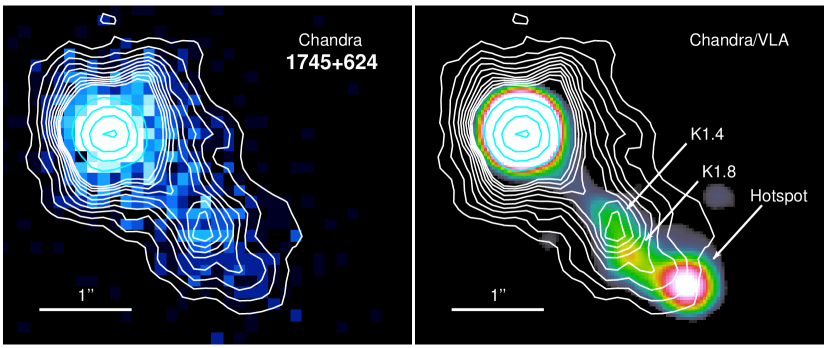
Figure 5: Smoothed Chandra X-ray contours plotted over the full band X-ray [left] and VLA 8.5 GHz [right] images (plotted logarithmically). The X-ray image was rebinned to 1/4th the native ACIS pixel size of 0.492^′′ and the outer contours are spaced by 0.5 counts/pixel from 0.5 to 5 counts/pixel. The main X-ray detected radio features (cf. Figure 4) are labeled.

2.3 Hubble Space Telescope

A deep Hubble Space Telescope (HST) image of 1745+624 was obtained from the STScI archive to search for optical emission from the jet. The data analyzed was taken with STIS using the CCD in CLEAR (unfiltered) imaging mode. This image is sensitive over a broad range in the optical band ($\sim$2,000–10,000 Å) with an effective wavelength of 5,740 Å. Four roughly equal exposures totaling just under 3,000 sec. (Table 1) were aligned, then cosmic-ray rejected and combined using the CRREJECT task in the STSDAS package in IRAF.

The quasar appears prominently in the image and has slightly saturated the inner few CCD pixels (the following description follows Figure 4 closely). In the vicinity of the radio jet, a faint resolved optical source is apparent just north of the jet (between K1.8 and the hot spot), but it is clearly unassociated with the extended radio source.

We modeled the central source with a series of elliptical isophotes using the ELLIPSE task in IRAF, successfully out to $\sim$1.2^′′. Other than a clear source $\sim$0.95^′′ roughly south of the quasar, this subtraction revealed the alluded to optical emission apparently coincident with K0.4. As this is adjacent to the central mildly saturated source, and similar features at two different position angles about the nucleus are also seen in the subtracted image (one is lined up with the direction of a diffraction spike), it is difficult to gauge its reality. It is formally a 5$\sigma$ detection in a 0.15^′′ radius circular aperture (contains 79$\%$ of encircled energy) in the central source subtracted image (Figure 4), where $\sigma$ here is the standard deviation in the background in apertures adjacent to the jet. Some of the optical emission may indeed originate from the radio source; its radio-to-optical spectra index of $\sim$1 (Table 2) is quite typical in quasar jets (Sambruna et al., 2004), so we tentatively identify it as an optical counterpart to the radio knot K0.4. This knot is unresolved from the nucleus in the Chandra image so is not discussed in the subsequent sections.

We analyzed the outer knots and hot spot similarly with 0.2^′′ radius apertures (87$\%$ encircled energy) centered on the radio positions in the unprocessed image and found no net positive signal. Measurements of the Poisson noise in these apertures result in a formal 3$\sigma$ point source detection limit of 0.01 $\mu$Jy. However, experience with similarly configured STIS CLEAR imaging data (Sambruna et al., 2004) allow us to more practically gauge detection limits for such jet knots – we favor the more conservative 3$\sigma$ limit of 0.06 $\mu$Jy derived from the previously published work.

An extinction correction of 10$\%$ was estimated using NED’s quoted values from the Schlegel, Finkbeiner, & Davis (1998) maps and though basically negligible, has been applied to the optical measurements (Table 2).

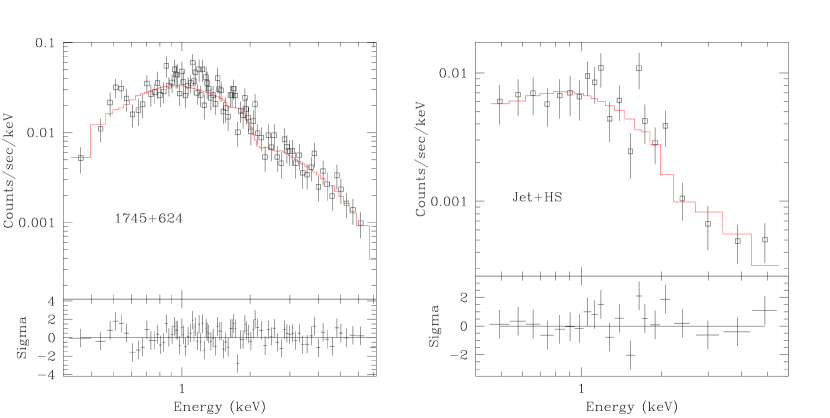
Figure 6: Top panels: Observed X-ray spectra of the core [left] and extended jet+hot spot [right] emission from 1745+624. The power-law plus absorption models are drawn as lines over the data (squares with error bars). Both models assumed a fixed local (galactic) absorption with an additional intrinsic ($z$=3.89) absorbing component allowed in the core spectrum (§ 2.4.1). The bottom panels show the residuals from the model.

2.4 Chandra X-ray Observatory

The quasar 1745+624 was observed with the ACIS camera aboard the Chandra X-ray Observatory (Weisskopf et al., 2002) and we retrieved this data from the Chandra archive. In this observation, the source was placed 30^′′ from the default aim-point position on the ACIS-S backside illuminated CCD, chip S3 (Proposers’ Observatory Guide, POG). The data were collected in a full readout mode of 6 CCDs resulting in 3.241 seconds readout time. The quasar’s count rate of 0.056 cts s^-1 gives 6-7$\%$ pileup in the core for this choice of the readout mode. After standard filtering, the effective exposure time for this observation was 18,312 sec (Table 1).

The X-ray data analysis was performed with the CIAO 3.2 software using calibration files from the CALDB3 database. We ran acis_process_events to remove pixel randomization and to obtain the highest resolution image data. The X-ray position of the quasar (R.A.= 17 46 14.057, Decl.= +62 26 54.79; J2000.0 equinox) agrees with the radio position to better than 0.2^′′, which is smaller than Chandra’s 90$\%$ pointing accuracy of 0.6^′′ (Weisskopf et al., 2002). The X-ray images were rebinned to 1/4 the native ACIS pixel-size of 0.492^′′ in the final image; the extended X-ray jet is already quite obvious in this image (Figure 5).

To determine the extent of the PSF at the location of the quasar, we ran a ray-trace using the Chandra Ray Tracer (CHART) and then MARX to create a high S/N simulation of a point source. We modeled the quasar core as a point source with the energy spectrum given by the spectral fitting described below. For the simulation, we added 7$\%$ errors to account for uncertainty in the ray-trace model (Schwartz et al., 2000b; Jerius et al., 2004). We then extracted a radial profile from both the Chandra data and the simulated point source image assuming annuli separated by 0.45^′′ and centered on the quasar. The PSF was normalized to match the peak surface brightness of the core.

A comparison between the quasar profile and the simulated PSF shows an excess of counts above the PSF beginning at $\sim 1.2$^′′ from the quasar centroid. Therefore, in our analysis of the quasar’s core X-ray emission (§ 2.4.1), we define a 1.2^′′ radius circular region centered on the X-ray centroid which excludes any overlap with the region defined for the extended jet. For our analysis of the extended emission (§ 2.4.2), we defined two pie-shaped regions based on the radio images – one for the jet, and another for the terminal hot spot. Spectral analysis was performed in Sherpa (Freeman et al., 2001) using counts in the energy range 0.3–7 keV.

Figure 7: [left] Integrated radio spectrum of 1745+624 along with the hot spot and jet emission spectra from this work. Lines are best fit power-laws to the hot spot and jet data. Integrated measurements are at 38 (Hales et al., 1995), 74 (VLSS; Cohen et al., 2006), 151 (Hales et al., 1993; Visser et al., 1995), 178 (Gower et al., 1967), 325 (Rengelink et al., 1997), 365 (Douglas et al., 1996), and 1400 MHz (Condon et al., 1998), and 2.3, 5, 8 GHz (Volvach et al., 2004), 8.5 and 15 GHz (this work). [right] Radio-to-X-ray spectral energy distributions of the total jet and hot spot emissions in 1745+624. The bowtie around the X-ray jet point represents the 1$\sigma$ measurement of the spectral slope (this is suppressed in the case of the hot spot because its X-ray spectrum is not well-constrained).

2.4.1 The Quasar Core X-ray Emission

Based on the PSF analysis described above, a 1.2^′′ radius circular region encircles about 91$\%$ of the total quasar counts. A total of 1,132 counts are detected in this region corresponding to 1,107.6$\pm 34.1$ net counts. We fit the spectrum between 0.3 and 7 keV with an absorbed power law model assuming the photoelectric absorption model with abundance tables from Anders & Grevesse (1989). Our analysis included the pileup model specified by Davis (2001), which gives the fraction of piled photons within 6–9$\%$. The best-fit power law model has a photon index, $\Gamma_{\rm X}=1.85^{+0.07}_{-0.12}$ and a total absorbing Hydrogen column of $N_{\rm H}=1.27^{+0.27}_{-0.25}\times 10^{21}$ cm^-2 for an absorber at $z$=0 ($\chi^{2}=77.8/82$ dof, and we give 1$\sigma$ errors for one significant parameter). Note that the fitted column is greater than the equivalent column within the Galaxy (3.3$\times 10^{20}$ cm^-2) in the direction of the quasar at high significance. This model gives a 0.5–2 keV flux of 1.5$\pm 0.2\times 10^{-13}$ erg cm^-2 s^-1 and 2–10 keV flux of 3.0$\pm 0.3\times 10^{-13}$ erg cm^-2 s^-1 for the core.

If we now assume that the quasar spectrum is absorbed by two absorption components, a known (and fixed) Galactic column at $z$=0 and an intrinsic absorber located at the quasar redshift, $z$=3.89, we obtain an intrinsic $N_{\rm H}=2.35^{+0.78}_{-0.71}\times 10^{22}$ cm^-2 and the best-fit photon index of $\Gamma_{\rm X}=1.74^{+0.08}_{-0.14}$ ($\chi^{2}$=78.5/82 dof); see Figure 6. This large intrinsic absorption column confirms the previous ASCA result from analysis of the total emission (Kubo et al., 1997) and is in agreement with the average column observed in samples of high-redshift radio-loud quasars (Bassett et al., 2004). These are comparable to the absorptions observed in broad absorption line (BAL) quasars (Brotherton et al., 2005), where it is usually associated with an outflow. The photon index is also typical of that observed in lower redshift quasars with X-ray jet detections (e.g., Gambill et al., 2003). In this model, the 0.5–2 keV and 2–10 keV fluxes are equal to 1.6$\pm 0.2\times 10^{-13}$ erg cm^-2 s^-1 and 3.4$\pm 0.2\times 10^{-13}$ erg cm^-2 s^-1, respectively; these correspond to quasar X-ray luminosities, $L_{\rm X}$(0.5–2 keV) = 1.6$\times 10^{46}$ erg s^-1 and $L_{\rm X}$(2–10 keV)=5.7$\times 10^{46}$ erg s^-1 (unabsorbed and K-corrected).

We determined that there is no Fe-line present in the quasar spectrum with a 3$\sigma$ upper limit on the equivalent width of 210 eV, consistent with previous ASCA results (Kubo et al., 1997). The Chandra data are also consistent with little or no variability in both the X-ray flux and spectrum since previous observations of (the total emission from) the quasar (Fink & Briel, 1993; Kubo et al., 1997).

2.4.2 The Extended X-ray Emission

We extracted the spectrum of the total extended X-ray emission (from the jet and hot spot) assuming a pie-shaped region between 1^′′ to 2.75^′′ centered on the quasar core. The assumed background region was equal to a pie region spanning the same radii, but excluding the jet+HS region. A total of 241 counts corresponding to 224.5$\pm 15.4$ net counts was detected in this region. The binned spectrum was fit with an absorbed power law model, and the best fit photon index for a fixed Galactic column is equal to $\Gamma_{\rm X}=1.71^{+0.13}_{-0.12}$ ($\chi^{2}$=17.9/19 dof). This gives a 0.5–2 keV flux of 3.1$\pm 0.3\times 10^{-14}$ erg cm^-2 s^-1, and 2–10 keV flux of 6.1$\pm 0.6\times 10^{-14}$ erg cm^-2 s^-1 (Figure 6).

Since we found that the radio hot spot spectrum is significantly steeper than that of the jet (§ 2.5), we attempted to analyze the jet and hot spot emissions separately, assuming pie-shaped regions between 1^′′ to 2.05^′′ and 2.05^′′ to 2.75^′′, respectively, centered on the quasar core. The background region was equal to the annulus with the same radii excluding the jet and hot spot regions. A total of 181 counts were detected in the jet region which result in 173.2$\pm 13.7$ net counts. We binned the spectrum to have a minimum of S/N=3 and fit an absorbed power law model to the jet spectrum within the 0.3–7 keV energy range assuming the Galactic equivalent Hydrogen column of 3.3$\times 10^{20}$ cm^-2. We obtain the best fit photon index $\Gamma_{\rm X}=1.62^{+0.16}_{-0.17}$ ($\chi^{2}$= 10.1/14 dof) corresponding to a 0.5-2 keV flux of 2.2$\pm 0.2\times 10^{-14}$ erg cm^-2 s^-1 and 2-10 keV flux of 5.1$\pm 0.5\times 10^{-14}$ erg cm^-2 s^-1. Similarly, for the hot spot (net 29$\pm$6.4 counts only), we found $\Gamma_{\rm X}=2.1\pm 0.6$ (1$\sigma$) and fluxes 6.9$\times 10^{-15}$ erg cm^-2 s^-1 (0.5–2 keV) and 7.9$\times 10^{-15}$ erg cm^-2 s^-1 (2–10 keV). These results suggest that, as in the radio band, the hot spot’s X-ray spectrum is steeper than the jet, although the formal difference is not well determined because of the large uncertainty in the hot spot spectrum ($\Gamma^{\rm HS}_{\rm X}-\Gamma^{\rm Jet}_{\rm X}$=0.5$\pm$0.6). The model results from this paragraph are the ones used in the subsequent discussion.

We also allowed the total absorption column of the jet emission to vary and obtained a slightly steeper photon index $\Gamma_{\rm X}=1.74^{+0.36}_{-0.33}$ and a 3$\sigma$ upper limit to the absorption column of $<2\times 10^{21}$ cm^-2. This fitted photon index is consistent within 1$\sigma$ of the value found with the column fixed. We thus conclude that there is little gained by allowing the column to vary.

In the Chandra image, the X-ray intensity ratio of the knots K1.4 to K1.8 is $\sim$0.6:0.4. Assuming that the X-ray spectrum does not change drastically between these two regions (there is no significant difference in radio spectra; § 2.5), we estimated their fluxes using their respective ratios of the total flux (Table 2).

2.5 Assessment of the Broad-band Jet Spectra

Taking our flux measurements of the hot spot at the four radio frequencies, we fit a spectral index of $\alpha$=1.28$\pm$0.10 ($F_{\nu}\propto\nu^{-\alpha}$), compared to $\alpha$=1.45 measured by Becker, Helfand, & White (1992) from mostly the same data (Tables 1 & 2; Figure 7). In comparison to the individual jet knot measurements (below), we believe this result is more robust because the hot spot is bright, compact, and well-detected at the observed frequencies. The fitted spectral index is insensitive to the presented low resolution 1.5 GHz measurement ($\alpha$=1.29$\pm$0.15 omitting this measurement in the fit). This 1.5 GHz measurement though may be contaminated by emission from the adjacent K1.8 (Figure 2). Since the flux ratio of K1.8 to HS at the other bands is about 1:3, reducing the 1.5 GHz flux of the hot spot by 25$\%$ will change the spectrum to 1.20$\pm$0.09 which is still within the uncertainty.

The jet knots K1.4 and K1.8 are well-separated from the bright nucleus in the 5, 8.5 and 15 GHz images. These are the first reported detections of the jet at frequencies other than 5 GHz (Becker, Helfand, & White, 1992; Patnaik et al., 1992). We measured a ”total” jet spectral index of 0.95$\pm$0.18 between these 3 frequencies on the maps reconvolved to a common 0.35^′′ beam (§ 2.2). Spectral indices measured from the full-resolution images give larger uncertainties (Table 2) because the signal-to-noise ratio of the individual jet knot detections are low. Including the “super-resolved” 1.5 GHz image, the resultant 4-frequency radio spectral index is 0.93$\pm$0.09, which we adopt as the best determined spectral index of the jet (Table 2; Figure 7).

The overall impression is that the jet knot radio spectra are fairly steep – on the steep end of what is observed in more nearby examples (Bridle & Perley, 1984). As indicated by previous work (Becker, Helfand, & White, 1992), the hot spot radio spectrum is significantly steeper than the jet ($\alpha_{\rm HS}$-$\alpha_{\rm jet}$=0.35) and this is also suggested to be the case in the X-ray data (§ 2.4.2). The slope of the hot spot spectrum is as steep as the kpc-scale feature detected in GB 1508+5714 (Cheung et al., 2005b, 2006) and is similar to those measured in comparably high-redshift radio galaxies (e.g., De Breuck et al., 2001, and references therein). These steep radio spectra are probably due to a combination of the increased importance of IC/CMB losses on the higher energy electron population and higher $(1+z)$ rest-frame frequencies sampled by the observations – this effect may be important when comparing low and high-redshift jets (§ 3.2.4).

In addition to the radio spectra, the optical upper limits of all the extended features preclude a simple power-law extrapolation of the radio data into the X-ray band (i.e., $\alpha_{\rm r}$ and $\alpha_{\rm ro}>\alpha_{\rm rx}$; Figure 7). This behavior is common among the X-ray detected jets in quasars (e.g., Sambruna et al., 2004). One should bear in mind that this assumes that the radio-to-X-ray radiation all originate in the same emitting region, and also, the optical limits assumed a point source. Though the radio knots are unresolved at $\sim$0.15–0.2^′′ resolution (§ 2.2), it does not preclude the optical emission being more extended or that there are multiple emitting components.

Although there are complicating factors in the measurements of the radio and X-ray spectra as discussed above, our analysis suggests that the power-law slopes measured in the two bands are different for the jet. Formally, this difference, $\alpha_{\rm r}-\alpha_{\rm x}$=0.31$\pm$0.19, is significant. No similar evidence is evident in the hot spot spectra, as we are limited by the low statistics of its X-ray detection.

3 Discussion

At $z$=3.89, the 1745+624 system displays a fully formed jet as observed by us when the Universe was only about 12$\%$ of its present age. For its projected length $L=18$ kpc, and assuming a constant hot spot advance velocity $\beta_{\rm adv}\sim 0.1-1$ (see in this context Scheuer, 1995, but also comments at the end of § 3.3), the lifetime of the radio source is roughly $t_{\rm life}\sim L/(\beta_{\rm adv}c\,\sin\theta)\sim$ Myr (the jet viewing angle $\theta\sim 10\hbox{${}^{\circ}$}$ is taken here for illustration; see below). This structure signals long-term active accretion at a very early cosmic epoch, along with a roughly stable black hole/accretion disk axis (e.g., Begelman, Blandford, & Rees, 1984). Such large-scale jets (deprojected $\sim$100 kpc in this case) at high-redshifts are not necessarily rare, though they have not been systematically searched for and studied. Cheung et al. (2005b, and manuscript in preparation) has only recently identified $\sim$10 other jets on a comparable scale in a VLA study of a sample of $z>$3.4 (out to $z$=4.7) flat-spectrum-core radio sources; 1745+624 remains the most radio-luminous example observed (§ 1).

Despite the extreme luminosity of the jet in 1745+624, its extended radio and X-ray emissions appear quite similar to other more local examples in regard to its morphology, spectral energy distribution, and radio polarization. This is quite surprising as higher-$z$ jets have propagated through the (supposedly different) intergalactic medium of the early Universe (e.g., Rees, 1989). In the following, we first consider available evidence for relativistic beaming in the 1745+624 jet on both parsec and kpc-scales (§ 3.1). Then, we discuss the emission properties of the kpc-scale jet (§ 3.2) and the hot spot (§ 3.3), confronting the multiwavelength data with expectations from different emission models. Along the way, we make comparisons to other X-ray jets at low and high redshift. Finally, the broad-band data allow us to estimate the energetics of the jet, which we compare to the accretion parameters of the quasar nucleus (§ 3.4).

3.1 Radio Constraints on Relativistic Beaming of the Jet

Several lines of evidence suggest that relativistic beaming in the 1745+624 jet is significant on the observed scales. Both the radio (VLBI and VLA-scale) and X-ray structures appear one-sided to our detection limits. The best constraints on the sidedness comes from the presented 2.3 GHz USNO map (jet to counter-jet ratio $>$50; § 2.1) and proper motion studies with VLBI. Twelve epochs of higher resolution 8 GHz data from the same USNO program, obtained over $\sim$2.5 years (Piner et al., 2004), show a basically stationary inner ($\sim$1–1.5 mas distant) component, although velocities of a few $c$ are allowed by the formal fit (B.G. Piner, 2005, private communication). Maps from the Caltech-Jodrell Bank survey obtained over a longer time baseline at 5 GHz reveal three superluminal components presumably further down the jet (Taylor et al., 1994; Vermeulen et al., 2003, this is the highest redshift object in the sample – see Figure 1 in the latter). Converting to our adopted cosmology, their proper motions correspond to apparent speeds ranging from $\sim$6$c$ up to $\sim$16$c$. This restricts the maximum angle of the small-scale jet to our line of sight to be $<$7–19^∘.

The superluminal VLBI jet is oriented at PA$\sim$205–208^∘ in the sky (Taylor et al., 1994), increasing gradually to $\sim$216^∘ out to $\sim$110 mas (Figure 1; § 2.1). This further increases out to the visible arcsecond-scale structure (the hot spot PA=227^∘). The maximal (projected) changes in position angle between the different features is 6^∘ (cf. Table 2). The required intrinsic bend in the jet to account for these changing PAs is $\sim$6^∘ $\times\sin(20\hbox{${}^{\circ}$})$$\sim$2^∘, or even less (supposing the jet inclination $<$20^∘ as indicated by the proper motions).

Since we can trace the VLBI-scale emission out to the observed Chandra scales, the VLBI proper motions (and only small intrinsic bends) constrain the kiloparsec-scale jet to be aligned within $\;\buildrel<\over{\sim}\;$25^∘ to our line-of-sight, with a likely range of $\sim$10–20^∘, or less. Radio asymmetry studies of large scale quasar jets require jets like this to be relativistic ($\Gamma$$>$1, with strict upper limits of $\Gamma$$<$2–3; Wardle & Aaron, 1997); these constraints have bearing on the following discussion of the origin of the X-ray emission in the 1745+624 jet.

3.2 X-ray Emission Mechanisms in the Large-scale Jet

The absence of optical emission and the steep radio spectra of the jet knots in 1745+624 preclude a straightforward power-law extrapolation of the low energy (synchrotron) emission into the X-ray band (§ 2.5). The resultant convex broad-band spectral energy distribution (SED; Figure 7) is a common characteristic of X-ray emitting knots in the jets of powerful quasars (e.g., Schwartz et al., 2000a; Sambruna et al., 2004; Marshall et al., 2005; Harris & Krawczynski, 2006). As widely discussed, (unbeamed) inverse Compton emission also can not account for the observed excess of X-rays, and it is evident that this applies also to the present example at very high-redshift (§ 3.2.1). We explore the hypothesis that the bright X-ray emission is produced by relativistically beamed inverse-Compton scattering of the CMB photons (Tavecchio et al., 2000; Celotti, Ghisellini, & Chiaberge, 2001) as advocated by many workers. The main feature of this model is that in order to fulfill energy equipartition, significant beaming of the large-scale quasar jet emission is required (§ 3.2.2). “Non-standard” synchrotron models have also been proposed to reproduce the overall convex radio-to-X-ray SEDs and we discuss this possibility in § 3.2.3. The main difference between these models is the expected diverging redshift-dependence of the X-ray emission, and we discuss issues and prospects for distinguishing such a dependence from the observations (§ 3.2.4).

3.2.1 Basic Considerations

Generally, one can calculate the magnetic field in a synchrotron emitting radio source if we assume magnetic field energy equipartition with the radiating particles (corresponding to the minimum total energy of the system). In the 1745+624 radio jet, we use the observed radio properties of K1.4 and K1.8 (assuming negligible contribution from relativistic protons and no beaming, $\delta$=1) to calculate fairly high values of $B_{\rm eq,\,\delta=1}\approx 180$ $\mu$G and $200$ $\mu$G, respectively. These values are more than an order of magnitude higher (due to the exceptionally luminous nature of this radio jet; § 1) than those computed in lower-redshift quasar jets (Kataoka & Stawarz, 2005), but are comparable to values inferred for lower power FRI radio galaxies (Stawarz et al., 2006). The corresponding magnetic field energy densities of the knots, $U_{\rm B}=B_{\rm eq,\,\delta=1}^{2}/8\pi\approx 1.3-1.6\times 10^{-9}$ erg cm^-3, are $\sim$6–7 times greater than the CMB energy density at the quasar’s redshift, $U_{\rm CMB}=4\times 10^{-13}\,(1+z)^{4}$ erg cm^-3 $\approx 2.3\times 10^{-10}$ erg cm^-3. The latter quantity is, however, comparable to the energy densities of the knots’ synchrotron photons (in the case of sub-relativistic jet velocity),

$$U_{\rm syn}\approx{L_{\rm syn}\over 4\pi\,R^{2}\,c},$$ (1)

namely, $U_{\rm syn}\approx$ 2.8 and 3.8 $\times 10^{-10}$ erg cm^-3 for K1.4 and K1.8, respectively. In this estimate, we approximated the knots as spheres with radii, $R=0.2\hbox{${}^{\prime\prime}$}/2\approx 0.7$ kpc (§ 2.2), and took the synchrotron luminosities, $L_{\rm syn}\approx 10\times L_{\rm 5\,GHz}\approx 5-7\times 10^{44}$ erg s^-1, as appropriate for the radio continuum extending over a few decades in frequency with spectral index $\alpha_{\rm r}\approx 1$. For the spectral index $\alpha_{\rm r}\approx 1$, the expected X-ray flux densities ($F_{\rm X}$) from the synchrotron self-Compton (SSC) plus IC/CMB processes are simply:

$$F_{\rm X}^{\rm ssc}+F_{\rm X}^{\rm IC/CMB}\approx\left({\nu_{\rm r}\over\nu_{\rm X}}\right)\,\left({U_{\rm syn}+U_{\rm CMB}\over U_{\rm B}}\right)\,F_{\rm r}.$$ (2)

Using the 5 GHz radio flux measurements ($F_{\rm r}$), this severely underpredicts ($\sim$0.054 nJy (K1.4) and $\sim$0.074 nJy (K1.8) at 1 keV) the observed X-ray jet emission by factors of 87 and 42 in knots K1.4 and K1.8, respectively (Table 2).

3.2.2 Relativistic Beamed X-ray Emission?

The bulk velocity of kpc-scale quasar jets are likely to be at least mildly relativistic ($\Gamma>1$, Bridle et al., 1994; Wardle & Aaron, 1997). This can significantly influence the expected inverse Compton X-ray fluxes calculated above. Specifically, relativistic beaming ($\delta>1$) increases the IC/CMB emission, and decreases the SSC one. In 1745+624, the superluminal VLBI jet can be traced out to kpc-scales (§ 3.1), so the beamed IC/CMB X-ray emission will dominate over that produced by SSC in the visible jet. Assuming energy equipartition as an additional constraint, the expected IC/CMB flux is (for $\alpha\approx$1):

$$F_{\rm X}^{\rm IC/CMB}\approx\left({\delta\over\Gamma}\right)^{2}\left({\nu_{\rm r}\over\nu_{\rm X}}\right)\,\left({\Gamma^{2}\,U_{\rm CMB}\over\delta^{-10/7}\,U_{\rm B}}\right)\,F_{\rm r}\,\,\,\propto\,\,\,\delta^{24/7},$$ (3)

since in the jet rest frame (denoted by primes) $U^{\prime}_{\rm CMB}\approx\Gamma^{2}\,U_{\rm CMB}$, and the equipartition magnetic field $B^{\prime}_{\rm eq}=B_{\rm eq,\,\delta=1}\,\delta^{-5/7}$. Here, $\Gamma$ is the jet bulk Lorentz factor, and $U_{B}=B_{\rm eq,\,\delta=1}^{2}/8\pi$. This gives the required $\delta=4.6$ and 3.9 for the knots K1.4 and K1.8, respectively, to explain the observed X-rays via inverse Compton emission. In this interpretation, the (small) decrease of the required Doppler factor along the jet is a direct consequence of the fading X-rays with the corresponding brightening of the radio emission (Figure 5; cf. similar multi-wavelength morphologies in other well-studied jets like, 3C 273 (Marshall et al., 2001; Sambruna et al., 2001), 0827+243 (Jorstad & Marscher, 2004), PKS 1127–145 (Siemiginowska et al., 2002), and PKS 1136–135 (Sambruna et al., 2006)).

Although there is evidence that the 1745+624 jet is highly relativistic on parsec scales (§ 3.1), there are few independent constraints (the one-sidedness of the radio and X-ray jets) to directly support the fairly high Doppler factors on these large scales, as implied in this interpretation. The inferred Doppler factors require minimum Lorentz factors, $\Gamma\geq(\delta+\delta^{-1})/2$ = 2.4 (K1.4) and 2.1 (K1.8). These approach the strict upper limits on the speeds of large-scale quasar jets deduced from radio asymmetry studies ($\Gamma$$<$2–3; Wardle & Aaron, 1997). If we assume the 1745+624 jet flow is moving near these maximal values, the derived Doppler factors require that the jet is inclined within $\;\buildrel<\over{\sim}\;$12–15^∘ to our line of sight, in agreement with the values inferred in § 3.1. Given the discussed Lorentz factors of $\sim$2–3, the Doppler factor is fairly insensitive to jet angles considered; for instance, $\delta$=5.5–3.6 ($\Gamma$=3) and $\delta$=4.0–3.2 ($\Gamma$=2.1) for jet angles, $\theta$=0^∘–15^∘. Thus we can just plausibly explain the level of X-ray jet emission in this jet via the IC/CMB mechanism if we push the speeds to be consistent with upper limits inferred from previous studies, together with the small viewing angles. It should be stressed that these estimates assumed a single-zone emitting region, and there are generally more free parameters in both Compton and synchrotron models invoking substructure in the jet (e.g., Celotti, Ghisellini, & Chiaberge, 2001; Stawarz & Ostrowski, 2002; Siemiginowska et al., 2006).

Related to the beaming issue, we should remark that the observed radio power of the 1745+624 jet (excluding the hot spot region) is very large, $L_{\rm 5\,GHz}\approx 10^{44}$ erg s^-1, suggesting its synchrotron luminosity of order $\sim 10^{45}$ erg s^-1 or greater. Such enormous radio powers from large-scale jets (exclusive from extended radio lobes) are quite extreme, so invoking even moderate beaming factors would reduce the intrinsic jet frame luminosity (by 1–2 orders of magnitude) to more comfortable levels.

This relativistically beamed IC/CMB model also requires that there is a sufficient number density of low energy electrons to upscatter CMB photons into the observed Chandra band. Radio emission would be radiated by these electrons at very low-frequencies (10’s MHz in this case) and subarcsecond-resolution radio imaging capabilities at these energies are not widely available. Curiously, Stickel (1993) noticed that the integrated radio spectrum of 1745+624 contains a steep-spectrum excess at low-frequencies; this quasar would be catalogued as a steep-spectrum radio quasar in low-frequency surveys and/or if it were local (the $1+z$ shift in observed frequencies). In our own compilation of radio data from the literature (Figure 7), we find $\alpha$=0.55$\pm$0.01 from 38 MHz to 1.4 GHz and $\alpha$$\sim$0 at the higher frequencies where our imaging observations were taken. If we extrapolate the observed individual spectra of the (dominant $\alpha$$\sim$0) core and steep-spectrum extended component to lower frequencies, it implies that the latter dominates the total low-frequency emission. The well-studied $z$=0.158 quasar 3C 273 shows a similar low-frequency excess apparent down to $\sim$10’s MHz (Courvoisier, 1998) and resolved low-frequency imaging shows its extended X-ray emitting (e.g., Marshall et al., 2001; Sambruna et al., 2001; Jester et al., 2006) radio jet does indeed dominate the total flux at low frequencies (cf. figure A1 in Conway et al., 1993). Further, although this low-frequency emission in 1745+624 is probably dominated by the (brighter and steeper spectrum at cm-wavelengths; § 3.3) hot spot, this does not preclude a low-frequency contribution from the jet. Interestingly, the X-ray spectral index of the jet (Table 2) matches the low-frequency integrated radio one, as would be expected in the IC/CMB scenario. Future low-frequency imaging observations can clarify this by showing the relative contributions of the jet and hot spot in this and similar systems (see Harris, 2006, for future prospects).

3.2.3 Synchrotron Models for the X-ray Emission

In lieu of the beamed IC/CMB interpretation, synchrotron models with non-standard and/or multiple electron components are able to account for the “excess” X-ray emission (Dermer & Atoyan, 2002; Stawarz & Ostrowski, 2002; Stawarz et al., 2004; Jorstad & Marscher, 2004). These models are attractive because in nearby low-power FRI jets, it is widely believed that synchrotron X-ray emission is produced (e.g., Harris & Krawczynski, 2006), although they do not show the same convex SEDs, and emit at much smaller (few kpc) scales than the discussed quasar jets (10’s–100’s kpc scales). The challenge remains to explain the strong upturn in the X-ray band (i.e., the small values of $\alpha_{\rm ox}$) observed in powerful jets such as in 1745+624.

While it is true that an increased energy density of the CMB photons at $z>1$ will result in a stronger radiative cooling of the ultra-relativistic electrons, the maximum electron energy available assuming efficient (although realistic) continuous acceleration process is still high enough to allow for production of an appreciable level of keV synchrotron photons. In the case of the 1745+624 jet, the comoving energy density of the magnetic field (by assumption close to equipartition with the radiating electrons, as given above) is lower than the comoving energy density of the CMB photons, $U^{\prime}_{\rm B}<U^{\prime}_{\rm cmb}$, if only $\delta^{5/7}\Gamma>2.5$. Thus, assuming even very moderate bulk velocity and beaming, the jet electrons cool mainly by inverse-Comptonization of the CMB photon field. In the equipartition derived magnetic field of $B$=200 $\mu{\rm G}$, the electrons emitting the highest energy photons detected ($\sim$6 keV, observed) have electron energies, $\gamma=E_{\rm e}/m_{\rm e}c^{2}=(\nu_{\rm Hz}(1+z)/\delta B_{\rm\mu{\rm G}})^{1/2}\sim 10^{8}$. Since their cooling are dominated by inverse Compton losses, the appropriate timescale can be evaluated roughly as $t_{\rm cool}^{\prime}=3\,m_{e}\,c/4\sigma_{\rm T}\gamma U_{\rm CMB}^{\prime}\sim 4.4$ yrs. This evaluation is rough, because in fact the considered high energy electrons are expected to radiate in a transition between Thomson and Klein-Nishina cooling regimes, since

$$\left({\Gamma\,\varepsilon_{\rm cmb}\over m_{\rm e}c^{2}}\right)\,\left({E_{\rm keV}\over m_{\rm e}c^{2}}\right)\sim 1\,,$$ (4)

with the energy of the CMB photon $\varepsilon_{\rm cmb}\approx(1+z)$ milli-eV, and the jet bulk Lorentz factor $\Gamma$ of the order of a few (see in this context Dermer & Atoyan, 2002). For such parameters and the considered electron energies, the ‘optimistic’ electron acceleration timescale $t^{\prime}_{\rm acc}\sim\zeta\,r_{\rm g}/c\sim 0.01$ yr, where $r_{\rm g}$ is the electron gyroradius and $\zeta\sim 10$ is the efficiency factor depending on the jet plasma conditions (see Aharonian et al., 2002). This is still much shorter than the timescale for radiative losses, while the latter is order of magnitudes longer than the timescale for the electron escape from the emission region.

The postulated stochastic acceleration mechanism can produce a flat-spectrum high-energy electron component, with the total energy density not exceeding the magnetic field energy density (see Stawarz & Ostrowski, 2002, for a discussion). The observed synchrotron spectrum of such particles (from the unresolved emitting region) is expected to show a spectral index modified (increased) by the radiative losses. With the condition of continuous injection of freshly accelerated electrons (characterized by a power-law energy spectrum $n^{\prime}(\gamma)\propto\gamma^{-p}$), such a spectral index would be $\alpha=0.5$ for any electron index $p<2$ (see Heavens & Meisenheimer, 1987), which is very close to the observed X-ray spectral index ($\alpha_{\rm X}\approx 0.62^{+0.16}_{-0.17}$) of the 1745+624 jet. Moreover, the total luminosity of such a high-energy synchrotron component, if indeed limited only by the energy equipartition requirement, should be comparable to or less than the luminosity of the low-energy (radio) synchrotron component. That is in fact the case, since the total $1$ keV luminosity of the 1745+624 jet (excluding the terminal feature discussed in § 3.3) is $\sim 3\times 10^{45}$ erg s^-1 while, as we argue in § 3.2.1 above, the radio jet luminosity is $>10^{45}$ erg s^-1. Note, that in the framework of this synchrotron interpretation, the X-ray-to-radio jet luminosity ratio is not expected to change systematically with redshift in contrast to expectations in an IC/CMB interpretation, and this issue is discussed in the next subsection.

3.2.4 Redshift Dependence of the X-ray Emission?

The simplest versions of synchrotron and IC/CMB models give significantly different predictions for the X-ray jet emission at high redshift because of the strong increase of the CMB energy density $\propto(1+z)^{4}$ (e.g., Schwartz, 2002). With all else equal, they predict divergences in the observed X-ray to radio monochromatic luminosity ($f_{\nu}=\nu\,F_{\nu}$) ratio, $f_{\rm x}$/$f_{\rm r}$ exceeding a factor of 100 or more at $z$$>$2 (cf. Equation 3). This difference should be readily apparent in observations of $z\sim$4 jets like in 1745+624 if the X-rays were dominated by IC/CMB emission. X-ray jets detected so far have observed $f_{\rm x}$/$f_{\rm r}$ values which range over 4 orders of magnitude and there is no obvious sign of a $(1+z)$-dependence in the latest large compilation of Kataoka & Stawarz (2005).

However, there are complicating factors which will skew such correlations, in both models, such as source-to-source (and knot-to-knot within a single jet) variations in jet magnetic fields, electron energy densities, and speeds. Particularly in current samples biased toward “blazars”, the X-ray jet emission is particularly sensitive to the (very small) jet angles to our line of sight if there is significant relativistic beaming on these large scales. For an IC/CMB origin, Cheung (2004, cf. figure 4 therein) outlined such a scenario to account for the large $f_{\rm X}/f_{\rm r}$ ratio of the $z$=4.3 GB 1508+5714 quasar jet ($>$ 100; among the largest value found thus far) in comparison to other known, lower redshift ($z\lower 2.15277pt\hbox{$\;\buildrel<\over{\sim}\;$}$2) jets due mostly to its extreme redshift. This scenario can be extended to the $z$=3.63 core-dominated quasar J2219–2719 where 6 total extended X-ray counts were recently detected in an $\sim$8 ksec exposure (Lopez et al., 2006), and can be attributed to a $\sim$1 mJy radio feature 2^′′ south of the quasar (thus $f_{\rm X}/f_{\rm r}>100$ also; Cheung et al., 2005b, and manuscript in preparation). Two quasars showing particularly low $f_{\rm x}/f_{\rm r}$ ratios, despite their fairly high-redshifts ($z$=1.4 and 2) also stood out – these are especially lobe-dominated quasars in comparison to the other examples, and a connection to beaming was suggested (see Cheung, 2004, for a discussion).

One caveat to note is that the Doppler factors required for the knots in the 1745+624 jet (in the minimum-energy + IC/CMB framework) are rather moderate, $\delta=4-5$, and similar to that found in the GB 1508+5714 case (Cheung, 2004, § 1). The required $\delta$ in these two $z\sim$4 quasar jets are at the low end of the corresponding values calculated for lower-redshift objects ($\delta\sim$4–25). In fact, these few critical data points at high-$z$ help to define the trend discussed by Kataoka & Stawarz (2005, figure 10 therein) that the maximal values of $\delta$ required to explain the X-ray jet emission as IC/CMB decreases with redshift. Also, in contrast to the GB 1508+5714 and J2219–2719 cases, the $f_{\rm x}$/$f_{\rm r}$ values of the 1745+624 jet are closer to those observed at lower-redshifts (Table 2 and footnote 9). Although second-order effects from the intrinsic jet properties should be factored in, the low implied jet Doppler factors and lack of a very obvious redshift-dependence of $f_{\rm x}$/$f_{\rm r}$, can be taken as evidence against an IC/CMB interpretation. In particular, if there were more extreme Doppler factors than in the $z$$\sim$4 quasars observed so far, the large-scale jets would be orders of magnitude brighter and will outshine the active cores in X-rays via the IC/CMB process (Schwartz, 2002). Currently however, no such sources have been found in a growing number of high-$z$ radio-loud quasars imaged with subarcsecond-resolution by Chandra (Bassett et al., 2004; Lopez et al., 2006), so where are the very highly beamed high-$z$ X-ray jets? There is of course a natural Malmquist bias inherent in studying very high-redshift objects, so this and other selection biases must be addressed in future samples.

On the other hand, if these trends persist with further observations, it may instead reflect intrinsic differences between large-scale quasar jets located at different redshifts and/or their different environments, which are then probed with observations. For example, in the IC/CMB interpretation, the trend may imply that high-$z$ jets of this kind are intrinsically slower than their lower-redshift counterparts. This may be due to a more disturbed environment (evidenced by the “alignment effect” of high-$z$ radio galaxies; e.g., Rees 1989) through which high-$z$ jets are propagating. Such an scenario, in fact, was suggested early on to explain the distorted morphologies observed in a large samples of high-$z$ ($\sim$1.5–3) quasars and radio galaxies (e.g., Barthel et al., 1988).

As current X-ray studies have tended toward known well-studied radio jets (e.g., Sambruna et al., 2004; Marshall et al., 2005) that are relatively local, it is important to test if this and other trends persist and can be clarified with larger, more homogenous samples of distant ($z>$2–4) jets. In analogy to VLBI proper motion studies, the earliest superluminal motions detected tended to be the highest (Vermeulen & Cohen, 1994) and larger ensembles of source measurements now tend toward lower values (Vermeulen et al., 2003; Kellermann et al., 2004). This may mean that beaming factors of kpc-scale X-ray jets as inferred from IC/CMB calculations are more typically smaller than the highest ones found thus far.

3.3 The Terminal “Hot Spot”

Recent Chandra studies have aimed to distinguish the X-ray detected terminal jet features (i.e., the hot spots) from the jets (Hardcastle et al., 2004; Kataoka & Stawarz, 2005; Tavecchio et al., 2005). Many of these knots show much the same problem as in the jet, i.e. the inability to extrapolate the radio-to-optical power-law slopes smoothly in the X-ray band, and the underprediction of not-beamed inverse-Compton (SSC and IC/CMB) emission to the observed. In this context, it is useful to discuss the terminal feature K2.5 of the 1745+624 jet as a terminal hot spot.

Knot K2.5 follows the conventional empirical definition of a hot spot only loosely (Bridle et al., 1994), as applying these strict criteria to such high-redshift, small angular-size jets is quite restrictive. Hot spots are strong terminal shocks formed at the tips of powerful jets where the strong compression of the jet magnetic field leads to a transverse configuration and relatively high radio polarization. This expectation is in good agreement with observations of sources located at low redshifts. K2.5 is situated at the edge of the radio source and it is indeed compact with a spatial extent of $\sim 0.15\hbox{${}^{\prime\prime}$}\times 0.075\hbox{${}^{\prime\prime}$}\approx 1\times 0.5$ kpc (§ 2.2), which is typical for the known X-ray detected hot spots in quasars and FR II radio galaxies. However, the parallel configuration of the magnetic field with respect to the jet axis, as well its low degree of linear polarization relative to the rest of the jet (Figure 3), are not expected, nor typical of the hot spots resolved in more nearby radio sources (Bridle & Perley, 1984). This may betray the dominance of an underlying jet flow in this feature.

The 5 GHz flux of the hot spot in 1745+624 implies a monochromatic luminosity, $L_{\rm 5\,GHz}\approx 2.42\times 10^{44}$ erg s^-1. This is higher, although still comparable to the 5 GHz luminosities of hot spots at lower redshifts (e.g., Kataoka & Stawarz, 2005). Assuming energy equipartition as in the jet, and a cylindrical geometry for the emitting region with radius $0.15\hbox{${}^{\prime\prime}$}/2\approx 0.5$ kpc (§ 2.2) and similar length, we calculate the hot spot magnetic field, $B_{\rm eq,\,\delta=1}\approx 660$ $\mu$G. This also is in rough agreement (though again slightly higher) with the minimum energy magnetic fields derived for the other knots (Kataoka & Stawarz, 2005).

The equipartition magnetic energy density of the hot spot, $U_{\rm B}\approx 1.7\times 10^{-8}$ erg cm^-3, is more than one order of magnitude greater than the energy density of the CMB radiation at the quasar’s redshift. However, the energy density of the synchrotron photons thereby, $U_{\rm syn}\approx 4.7\times 10^{-9}$ erg cm^-3, is roughly comparable to $U_{\rm B}$. In this evaluation, we took the hot spot radio spectral index, $\alpha_{\rm r}\approx 1$, its synchrotron luminosity $L_{\rm syn}\approx 10\times L_{\rm 5\,GHz}$, the geometry as described above, and neglected relativistic corrections. The implied 1 keV flux of the hot spot due to the SSC plus IC/CMB processes is then $\sim$0.18 nJy (Equation 2). As in the jet emission (§ 3.2.1), this is inconsistent with the observed X-ray flux, though here the deviation is less drastic (factor of $\sim$14; Table 2). However, one should keep in mind many of the underlying assumptions in such calculations before claiming a true disagreement between model predictions and the observations. In particular, the hot spot structure is in fact unresolved, hence a slightly smaller volume than considered, together with, e.g. small deviations from energy equipartition and spectral curvature (see below), could foreseeably bring the measurement into better agreement with the model prediction.

However, if we take the observed excess in X-rays over the estimated SSC flux at face value, this would not be the first such case for a hot spot. Hardcastle et al. (2004) has argued for a synchrotron origin of this X-ray excess in many local hot spot sources, though in the case of 1745+624, the optical upper limit precludes a straightforward extrapolation of the (very steep) radio spectrum up to the X-ray band. On the other hand, Tavecchio et al. (2005) has argued that there is an IC/CMB contribution from an underlying relativistic portion of the jet terminus (unresolved by our observations) to the few X-ray detected hot spots studied in several $z\sim 1$ quasars.

The latter possibility is quite attractive in the case of 1745+624: as we noted earlier, the terminal jet feature in this source does not have typical hot spot-like radio polarization properties, and there could very well be an unresolved portion of the jet mixed in. If the multi-band radiative output of K2.5 is dominated by a relativistic jet flow, this would imply $\delta$=5 for an IC/CMB origin of the X-ray flux (using Equation 3 with all the parameters discussed above). This beaming factor is quite high, though comparable to values derived in lower-redshift quasars (Tavecchio et al., 2005). It is also slightly higher than the values obtained for the proper jet (knots K1.4 and K1.8; see § 3.2.2), though again, there are the usual uncertainties in these calculations to keep in mind. Regardless, the problem of terminal X-ray/radio knots in this and many quasar jets can be viewed as a simple extension of that in the jet knots.

One relevant issue in this discussion is the apparent lack of a hot spot on the side opposite of the nucleus to the prominent jet. If the advance speed of the jet is sub-relativistic, then some emission should have been visible on the counter-jet side. This can be reconciled by the fact that the usually inferred (sub-relativistic) advance speeds of hot spots in powerful radio sources assume that the jet thrust is balanced with the ram-pressure of the ambient material within a typical galaxy group/poor cluster environment (Begelman, Blandford, & Rees, 1984). However, if the jets propagate into the radio cocoon formed in a previous epoch of radio activity, i.e. in an environment with a substantially decreased number density and pressure, the advance velocity of the jet may be close to $c$. In such a case, combined Doppler and light-travel effects may result in an apparent lack of a visible counter hot spot. Such a scenario was proposed by Stawarz (2004) for the 3C 273 jet. Since the observed properties of 1745+624 and 3C 273 radio quasars are so similar, one could also apply this argument to explain the lack of emission visible on the counter-jet side in 1745+624.

Let us finally discuss yet another issue regarding this dominant radio feature, namely the extrapolation of its radio spectrum to lower frequencies. As discussed in § 3.2.2, an extrapolation of its observed $\sim$$1-10$ GHz continuum $\propto\nu^{-1.3}$ to lower frequencies exceeds the extrapolation of the flat-spectrum core component $\propto\nu^{0}$ at about $\sim 500$ MHz, and joins smoothly with the observed integrated low frequency emission at $\sim 200$ MHz (see Figure 7 [left]). In other words, one can attribute the $\sim$30–300 MHz integrated emission to the extended radio structure. Since the extended emission is probably dominated by the brightest feature, the hot spot (we can not exclude a contribution from the fainter inner jet; § 3.2.2), this would imply a broken power-law character of its synchrotron spectrum, $\propto\nu^{-0.5}$ for $\nu<300$ MHz and $\propto\nu^{-1.3}$ for $\nu>300$ MHz. In the standard continuous-injection model of terminal features in powerful jets (Heavens & Meisenheimer, 1987), the spectral break would correspond to the energies, $E_{\rm e}/m_{\rm e}c^{2}\sim 10^{3}$. This low-frequency break is expected in face of the large computed hot spot equipartition magnetic field, $B_{\rm eq,\,\delta=1}\approx 660$ $\mu$G (see a discussion in Brunetti et al., 2003; Cheung et al., 2005a).

3.4 The Jet Energetics

The multiwavelength emissions of the 1745+624 jet allow us to estimate the kinetic power of the outflowing plasma in this source. The kinetic power of the ultrarelativistic electrons and magnetic field characterizing the proper jet, under the minimum-power hypothesis, is roughly $L_{\rm j}\sim L_{\rm B}+L_{\rm e}\sim 2\times\pi R^{2}\,c\Gamma^{2}\,U^{\prime}_{\rm B}$, where $R\approx 0.7$ kpc is the jet radius and $U^{\prime}_{B}=1.5\times 10^{-9}\,\delta^{-10/7}$ erg s^-1 is the jet comoving magnetic field energy density, as discussed in § 3.2. Assuming for illustration, a jet viewing angle $\sim 10\hbox{${}^{\circ}$}$ (see § 3.1) and jet bulk Lorentz factor at the kpc-scale $\Gamma\sim 3$ (leading to the ‘comfortable’ value of the jet Doppler factor $\delta\sim 4.7$), one obtains a kinematic factor $\delta^{-10/7}\,\Gamma^{2}\sim 1$, and therefore a jet kinetic luminosity (regarding solely ultrarelativistic jet electrons and the jet magnetic field) $L_{\rm j}\sim 10^{45}$ erg s^-1.

If we regard the terminal feature as a “true” hot spot, we can estimate the kinetic energy of the jet. We approximate the broad-band synchrotron spectrum of the hot spot by a broken power-law: $\propto\nu^{-0.5}$ between the assumed minimum synchrotron frequency $\nu_{\rm min}=10$ MHz and the break frequency $\nu_{\rm br}=300$ MHz, followed by $\propto\nu^{-1.3}$ between $\nu_{\rm br}$ and the assumed maximum synchrotron frequency $\nu_{\rm max}=10^{12}$ Hz (see § 3.3). The radiative efficiency factor, i.e. the ratio of the power emitted by the hot spot electrons via synchrotron radiation, and the total power injected to these electrons at the terminal shock, is:

$$\eta_{\rm rad}\sim{\ln(\nu_{\rm max}/\nu_{\rm br})\over\ln(\nu_{\rm max}/\nu_{\rm min})}\sim 0.7\,.$$ (5)

The reconstructed radio continuum of the hot spot implies also its total synchrotron luminosity $L_{\rm syn}\approx 10\times L_{\rm 5\,GHz}\sim 2.5\times 10^{45}$ erg s^-1. Thus, the total kinetic power of the jet transported from the active center to the jet terminal point is roughly:

$$L_{\rm kin}\sim{L_{\rm syn}\over\eta_{\rm rad}\,\eta_{\rm e}}\,,$$ (6)

where $\eta_{\rm e}$ is the fraction of the jet kinetic energy transformed in the terminal shock to the internal energy of ultrarelativistic (i.e. synchrotron emitting) electrons. In the case of energy equipartition between the electrons and the magnetic field reached at the hot spot, one should expect very roughly $\eta_{\rm e}\sim 0.5$ (see Sikora, 2001, for a wider discussion). This gives $L_{\rm kin}\sim 0.75\times 10^{46}$ erg s^-1. In fact, $\eta_{\rm e}=0.5$ should be regarded as an upper limit, keeping in mind a possible proton contribution and work done by the outflow in pushing out the ambient medium, making $10^{46}$ erg s^-1 a safe lower limit for the kinetic power of the 1745+624 jet. The jet power estimated at the beginning of this subsection is an order of magnitude lower than its total kinetic power constrained from the hot spot emission. This may indicate a dynamical role of non-radiating jet particles (either cold electrons or protons; see in this context, Sikora & Madejski, 2000).

Let us compare the kinetic power of the 1745+624 jet estimated above with the accretion parameters of the quasar core. Due to the large distance of the quasar, and hence related observational difficulties, these accretion parameters cannot be evaluated precisely thus should be treated with some caution. Nevertheless, we note Stickel (1993) and Stickel & Kühr (1993) found a broad emission CIV line in the spectrum of the 1745+624 quasar at the observed wavelength $\lambda_{\rm CIV}^{\rm obs}=7553$ Å, and an observed ${\rm FWHM_{CIV}^{\rm obs}}=64.9$ Å. This gives the intrinsic velocity dispersion:

$$v_{\rm CIV}=c\,{{\rm FWHM_{CIV}}\over\lambda_{\rm CIV}}=c\,{{\rm FWHM_{CIV}^{\rm obs}}\over\lambda_{\rm CIV}^{\rm obs}}\approx 2576\,{\rm km\,s^{-1}}\,.$$ (7)

Stickel (1993) reported also a steep-spectrum ($\alpha_{\rm opt}=1.3$), non-variable and low-polarized optical continuum of the 1745+624 quasar, which we consider below as being produced by the circumnuclear gas solely. In other words, we assume that the host galaxy and the nuclear portion of the jet do not contribute significantly to the observed optical emission of the discussed object. At the observed wavelength $6600$ Å, corresponding to the source rest frame wavelength $1350$ Å, the detected continuum flux is $F_{6600}\approx 0.08$ mJy. Thus, the intrinsic continuum luminosity at the emitted frequency $1350$ Å, is simply $L_{1350}=4\pi d_{\rm L}^{2}\,\left[\lambda F_{\lambda}\right]_{6600}\approx 5.4\times 10^{46}$ erg s^-1. These estimates allow us to find the bolometric luminosity of the quasar core (assumed to be about ten times the $V$-band core luminosity), $L_{\rm bol}\sim 10\times L_{5500}\sim 10\,\left(\nu_{5500}/\nu_{1350}\right)^{1-\alpha_{\rm opt}}\,L_{1350}\sim 8.2\times 10^{47}$ erg s^-1, as well as the mass of the central supermassive black hole via the virial relation (Vestergaard, 2002; Vestergaard & Peterson, 2006):

$${{\cal M}_{\rm BH}\over{\cal M}_{\odot}}=5.4\times 10^{6}\,\left({v_{\rm CIV}\over 1000\,{\rm km/s}}\right)^{2}\,\left({L_{1350}\over 10^{44}\,{\rm erg/s}}\right)^{0.53}\lower 2.15277pt\hbox{$\;\buildrel>\over{\sim}\;$}1\times 10^{9}.$$ (8)

This can be taken as a lower limit in this case because the relation was calibrated for the broad component of the CIV line, which was not measured independently from the narrow one (Stickel, 1993; Stickel & Kühr, 1993); including the latter underestimates the measured broad-line width (Vestergaard, 2002) which could be $>$3,000 km s^-1. The corresponding Eddington luminosity is $L_{\rm Edd}\lower 2.15277pt\hbox{$\;\buildrel>\over{\sim}\;$}10^{47}$ erg s^-1 and the Eddington ratio, $\Lambda\sim L_{\rm bol}/L_{\rm Edd}\sim 1-10$. The latter is quite large and may indicate contribution of the emission due to an unresolved portion of the jet to the nuclear optical continuum produced by the accreting matter.

Finally, the total observed $1.4$ GHz flux of the 1745+624 radio source (780.6 mJy; Condon et al., 1998), gives the total monochromatic radio luminosity $L_{\rm R}\approx 1.6\times 10^{45}$ erg s^-1 thus a radio loudness parameter, ${\cal R}\sim 10^{5}\,L_{\rm R}/L_{\rm V}\sim 10^{3}-10^{4}$. Note that the discussed object, which possesses the most powerful observed radio jet known, is extremely ‘radio-loud’, as the standard division between radio-quiet and radio-loud sources (Kellermann et al., 1989) is ${\cal R}=10$. With the obtained values of the Eddington ratio and radio loudness, 1745+624 fits into the ‘radio-loud’ trend formed on the $\Lambda-{\cal R}$ plane by local ($z<0.5$) FR I radio galaxies and radio selected broad-line AGNs, as discussed in detail by Sikora, Stawarz, & Lasota (2006).

4 Summary

We have analyzed multi-frequency radio, optical and X-ray imaging data for the kpc-scale jet in the $z$=3.89 quasar 1745+624. This quasar hosts the most powerful large-scale radio and X-ray jet yet observed, with monochromatic radio and X-ray luminosities, $L_{\rm 5\,GHz}\approx 1.3\times 10^{44}$ erg s^-1 and $L_{\rm 1\,keV}\approx 2.8\times 10^{45}$ erg s^-1, respectively (excluding emission from the powerful terminal “hot spot”). Aside from its large radiative output, and related large inferred equipartition magnetic field (in comparison to local powerful jet sources), its properties (multi-wavelength morphology, radio polarization, and broad-band spectral energy distribution) are broadly similar to other lower-redshift quasar jets. This is unexpected in light of the dramatic increase in the CMB energy density and strong cosmic evolution of the intergalactic medium at such high-redshifts; this should have manifested in a dramatically different appearance of such large-scale outflows.

The spectral energy distributions of the resolved linear structures are discussed. In this jet, inverse-Compton scattered emission on the CMB photons can just account for the X-ray emission if the jet is inclined close to our line of sight ($\;\buildrel<\over{\sim}\;$10^∘) and if it is also moving relativistically, $\Gamma$=2–3. Several indirect arguments from the multi-scale radio observations of 1745+624 support such values of the large-scale jet kinematic parameters. The data are also consistent with a synchrotron interpretation provided the electron acceleration timescale is much shorter than that of the radiative losses, which we deem likely. The main distinguishing feature of the two models should manifest in drastically different X-ray/radio emission properties of such high-redshift jets though with only three current $z>$3 examples, no trends are yet apparent.

Via the virial relation, we estimate that a ${\cal M}_{\rm BH}\lower 2.15277pt\hbox{$\;\buildrel>\over{\sim}\;$}1\times 10^{9}\,{\cal M}_{\odot}$ supermassive black hole resides at the center of this galaxy. The broad-band emission of the extended components allow us to additionally estimate a jet kinetic power of $L_{\rm kin}\sim 10^{46}$ erg s^-1, which is a small fraction of the Eddington luminosity ($L_{\rm kin}/L_{\rm Edd}\sim 0.1$) corresponding to this black hole mass. As the bolometric luminosity of the quasar is $L_{\rm bol}/L_{\rm Edd}\sim 10$, the inferred jet kinetic power seems to be much less than the estimated accretion power. Despite this, the 1745+624 quasar, hosting the most powerful radio jet known, is extremely ‘radio-loud’ in comparison to more local radio selected quasars with a radio-loudness parameter ${\cal R}\geq 10^{3}$, and is surprisingly similar to local radio selected broad line AGNs regarding the accretion parameters.

Table 1: Multi-Telescope Archival Data for Quasar 1745+624

Instrument	Program	Date	Frequency	Exptime	Reference or Observer
(1)	(2)	(3)	(4)	(5)	(6)
VLA A-configuration	AB414	08-Sep-1991	1.5	500	Becker et al. (1992)
VLA A-configuration	AB414	08-Sep-1991	4.9	500	Becker et al. (1992)
VLA A-configuration	AP182	20-Feb-1990	8.5	100	Patnaik et al. (1992)
VLA B-configuration	AM303	08-Sep-1990	8.5	140	M. Malkan
VLA A-configuration	AB414	08-Sep-1991	14.9	810	Becker et al. (1992)
VLA B-configuration	AM303	08-Sep-1990	14.9	200	M. Malkan
VLA C-configuration	AM310	09-Dec-1990	14.9	200	M. Malkan
HST STIS 50CCD-CLEAR	8572	08-Sep-2000	5.2$\times$105	2,786	L. Storrie-Lombardi
Chandra ACIS-S3	4158	09-Sep-2003	0.3–7 keV	18,312	P. Strub

(1) Telescope, and array configuration or camera-aperture.
(2) Observational program code.
(3) Date of observation.
(4) Frequency of observations in units of gigahertz unless indicated otherwise.
(5) Total integration time in seconds. At 8.5 and 14.9 GHz, the multi-configuration data were combined.
(6) The program principal investigator is listed unless we located a published reference to the data.

Table 2: Multi-wavelength Flux Densities and Spectra of Extended Emission

Region	K0.4	K1.4	K1.8	K2.5 (hot spot)	Total Jet*
Distance (′′)	0.4	1.4	1.8	2.5	$\sim$0.8$-$2.0
PA (deg.)	221	224	221	227	225
$F_{\rm 1.5}$(mJy)	–	–	–	148.7$\pm$29.7	49.7$\pm$7.5
$F_{\rm 4.9}$(mJy)	–	6.8$\pm$1.0	9.3$\pm$1.4	32.3$\pm$3.2	17.6$\pm$1.8
$F_{\rm 8.5}$(mJy)	–	2.9$\pm$0.4	6.2$\pm$0.9	17.3$\pm$1.7	9.5$\pm$1.0
$F_{\rm 14.9}$(mJy)	3.4$\pm$0.7	3.0$\pm$0.6	2.5$\pm$0.5	7.5$\pm$1.1	6.4$\pm$1.0
$F_{\rm opt}$($\mu$Jy)	0.13(0.14)$\pm$0.03	$<$0.06(0.06)	$<$0.06(0.06)	$<$0.06(0.06)	–
$F_{\rm 1~{}keV}$(nJy)	–	4.7$\pm$0.5	3.1$\pm$0.4	2.5$\pm$0.6	7.8$\pm$0.8
$\alpha_{\rm r}$	–	0.96$\pm$0.33	1.15$\pm$0.20	1.28$\pm$0.10	0.93$\pm$0.09
$\alpha_{\rm ro}$	0.97(0.96)	$>$1.01(1.01)	$>$1.03(1.03)	$>$1.14(1.14)	–
$\alpha_{\rm rx}$	–	0.80	0.84	0.92	0.83
$\alpha_{\rm x}$	–	–	–	1.1$\pm$0.6	0.62${}^{+0.16}_{-0.17}$

Notes.—
–Knot names indicate their distances relative to the core in arcseconds. The position angle (PA) is positive east of north defined to be zero degrees.

–The flux densities, $F_{\nu}$, are at the radio frequencies 1.5, 4.9, 8.5, and 14.9 GHz, optical (opt; 5.2$\times$10⁵ GHz; extinction corrected values are indicated in parentheses), and 1 keV X-rays. For the hot spot and total jet, we converted the 2–10 keV fluxes from the spectral fits into flux density using the fitted spectral indices ($\alpha_{\rm x}$) indicated. The flux densities of the individual features come from the ratios of the (background subtracted) counts to the total jet, K1.4:K1.8 = 0.6:0.4.

–The radio ($\alpha_{\rm r}$), radio-to-optical ($\alpha_{\rm ro}$), radio-to-X-ray ($\alpha_{\rm rx}$), and X-ray ($\alpha_{\rm x}$; $\Gamma_{\rm X}=1+\alpha_{\rm X}$) spectral indices where $F_{\nu}\propto\nu^{-\alpha}$. The broad band spectral indices use 5 GHz values (for K0.4, the 15 GHz measurement was converted to 5 GHz assuming $\alpha_{\rm r}$=0.9).

*Jet fluxes in the radio were measured directly from the VLA maps. At 4.9, 8.5, and 14.9 GHz, the maps were reconvolved with a common 0.35^′′ beam with ($u,v$) tapering applied at the two higher frequencies. At 1.5 GHz, we used the super-resolved map (Figure 2).

References

- Aharonian et al. (2002) Aharonian, F. A., Belyanin, A. A., Derishev, E. V., Kocharovsky, V. V., & Kocharovsky, Vl. V. 2002, PhRvD, 66, 3005
- Aller et al. (2003) Aller, M. F., Aller, H. D., & Hughes, P. A. 2003, ApJ, 586, 33
- Anders & Grevesse (1989) Anders, E., & Grevesse, N. 1989, Geochim. Cosmochim. Acta, 53, 197
- Barthel et al. (1988) Barthel, P. D., Miley, G. K., Schilizzi, R. T., & Lonsdale, C. J. 1988, A&AS, 73, 515
- Bassett et al. (2004) Bassett, L. C., Brandt, W. N., Schneider, D. P., Vignali, C., Chartas, G., & Garmire, G. P. 2004, AJ, 128, 523