MPP-2006-76, LAPTH-1148/06
Probing cosmological parameters with the CMB: Forecasts from Monte Carlo simulations
Abstract
The Fisher matrix formalism has in recent times become the standard method for predicting the precision with which various cosmological parameters can be extracted from future data. This approach is fast, and generally returns accurate estimates for the parameter errors when the individual parameter likelihoods approximate a Gaussian distribution. However, where Gaussianity is not respected (due, for instance, to strong parameter degeneracies), the Fisher matrix formalism loses its reliability. In this paper, we compare the results of the Fisher matrix approach with those from Monte Carlo simulations. The latter method is based on the publicly available CosmoMC code, but uses synthetic realisations of data sets anticipated for future experiments. We focus on prospective cosmic microwave background (CMB) data from the Planck satellite, with or without CMB lensing information, and its implications for a minimal cosmological scenario with eight parameters and an extended model with eleven parameters. We show that in many cases, the projected sensitivities from the Fisher matrix and the Monte Carlo methods differ significantly, particularly in models with many parameters. Sensitivities to the neutrino mass and the dark matter fraction are especially susceptible to change.
1 Introduction
In the last few years precision measurements of the cosmic microwave background (CMB), large scale structure (LSS) of galaxies, and distant type Ia supernovae (SNIa) have helped to establish a new standard model of cosmology. In this model, the geometry is flat so that , and the total energy density is made up of matter (), and dark energy (, with equation of state ). With only a few free parameters this model provides an excellent fit to all current observations. Furthermore, each of these parameters is very tightly constrained by the observational data [1, 2, 3, 4, 5, 6].
However, many other parameters can plausibly have a physical influence on the cosmological data, even if their presence has not yet been detected. Such parameters are, for example, a running spectral index of the primordial power spectrum, an equation of state for the dark energy which differs from , and non-zero neutrino masses (e.g., [7, 8]). Indeed, neutrinos are already known to have non-zero masses from oscillation experiments, where strong evidence points to a mass in excess of eV for the heaviest mass eigenstate (see e.g. [9]). Given the sensitivities of future cosmological probes, even such a small mass will very likely be measured (e.g., [10, 11, 12, 13, 14, 15, 16, 17]). Thus, for future experiments such as the Planck satellite111ESA home page for the Planck project: http://astro.estec.esa.nl/SA-general/Projects/Planck/ and Planck-HFI web site: http://www.planck.fr/ and beyond, it will be necessary to include the neutrino mass in the data analysis.
When performing a parameter error forecast for future experiments, it is customary to use the Fisher matrix formalism in which the formal error bar on a given parameter can be estimated from the derivatives of the observables with respect to the model parameters around the best fit point [18, 19]. However, this approach can only give a reasonable estimation when the likelihood of the cosmological parameters approximates a multivariate Gaussian function of the cosmological parameters. In practice, significant departures from Gaussianity arise because of parameter degeneracies (in other words, because specific combinations of parameters are poorly constrained by the data), or because a parameter is defined in a finite interval, and its probability distribution does not fall to zero at one of the boundaries.
In this paper, we explore an alternative, simulation-based approach to derive projected sensitivities on the cosmological parameters for future experiments. This approach utilises synthetic data which emulate the expected instrumental and observational characteristics of the experiment under consideration. Using modern stochastic optimisation methods such as Markov Chain Monte Carlo or Importance Sampling [20], the projected parameter errors can be extracted from the synthetic data set in the same way that parameters are extracted from existing data. Since this technique makes no assumption about the Gaussianity or otherwise of the parameter probabilities, we expect it to be much more reliable than the conventional Fisher matrix forecast.
This simulation-based forecast technique is in principle applicable to any one cosmological probe or combination of probes of interest, provided that one can reliably synthesise the data set given some underlying cosmological model and the instrumental noise and sensitivity. In this work, we focus on the example of the Planck satellite, to be launched in 2007 or 2008 by ESA for measuring with unprecedented sensitivitiy the CMB temperature and polarisation anisotropies on the full sky [21] .
The paper is structured as follows. In section 2, we summarise the statistical properties of the CMB data, with or without lensing information, and illustrate how synthetic data can be generated for some given fiducial model and instrumental characteristics. Sections 3 and 4 outline, respectively, the simulation-based Monte Carlo Markov Chain method and the Fisher matrix formalism for forecasting cosmological parameter errors. Section 5 contains a detailed comparison of the results obtained using these two techniques for a minimal cosmological model with eight independent parameters. The analysis is extended in section 6 to a more complicated model with eleven parameters, a case in which the differences between the Monte Carlo and Fisher matrix results are exacerbated. We provide our conclusions in section 7.
2 CMB data model
Raw data from a CMB probe such as the Planck satellite can be optimally reduced to sky maps for the three observables of interest: the temperature and the two polarisation modes [22]. Maps are usually expanded in spherical harmonics, where the coefficients, or multipole moments, receive contributions from both the CMB signal and the experimental noise ,
| (2.1) |
Here, the index runs over (temperature), (curl-free polarisation), and (divergence-free polarisation). The noise part can be modelled as a combined effect of a Gaussian beam and a spatially uniform Gaussian white noise. Thus, for an experiment with some known beam width and sensitivity, the noise power spectrum can be approximated as
| (2.2) |
where is the full width at half maximum of the Gaussian beam, and is the root mean square of the instrumental noise. Non-diagonal noise terms (i.e., ) are expected to vanish since the noise contributions from different maps are uncorrelated. The assumption of a spatially uniform Gaussian noise spectrum ensures that the noise term is diagonal in the basis.
The signal contains ab initio various contributions from the primary anisotropies (related to primordial inhomogeneities on the last scattering surface), the secondary anisotropies (caused by the interaction of primary CMB photons with the intervening medium), and a wide variety of astrophysical foregrounds [23]. Since foreground emissions typically have non-thermal spectra (except for a small contribution of the kinetic Sunyaev–Zel’dovitch effect), they can be accurately removed by combining data from various frequency bands. After foreground cleaning, CMB maps should contain only the primary anisotropies, plus a few secondary effects such as the late integrated Sachs–Wolfe (ISW) effect and weak lensing distortions [24, 25, 26, 27] (both caused by the neighbouring distribution of dark matter and baryons) which do not alter the CMB’s Planckian shape. For the temperature and the -polarisation mode, the effect of weak lensing on is small and can be neglected in a first approximation (this is not true for the -mode, at least on small angular scales, or, equivalently, at large multipoles). Thus, for a full-sky experiment, each multipole moment and is an independent Gaussian variable. Since the signal is also uncorrelated with the noise, the power spectrum of the total (after foreground cleaning) reads
| (2.3) |
where the Dirac delta functions ensure that different and modes are uncorrelated.
A number of methods are available on the market for the extraction of the weak lensing deflection angle from the CMB signals; the role of weak lensing is to remap the direction of observation from to [28, 27]. These extraction methods exploit the non-Gaussian properties of the signal induced by lensing. The reconstructed deflection field can be specified by a single set of expansion coefficients in harmonic space, since in a first approximation the vector field is curl-free [28]. The field itself becomes non-Gaussian at low redshifts due to the non-linear evolution of the gravitational potential. However, at sufficiently large angular scales (i.e., ), contributions to the deflection field will come mainly from the linear regime. Thus, can be considered as an approximately Gaussian variable [29].
The power spectrum of the deflection field reads
| (2.4) |
where the noise power spectrum reflects the errors in the deflection map reconstruction, and can be estimated for a given combination of lensing extraction technique and experiment. Here, we refer to the quadratic estimator method of Hu & Okamoto [29], which provides five estimators of based on the correlations between five possible pairs of maps: , , , , . The estimator (from self-correlations in the -mode map) cannot be used in this method, because the -mode signal is dominated by lensing on small scales. The authors of [29] also provide an algorithm for estimating given some hypothetical observed power spectra . This final noise power spectrum corresponds to the minimal noise spectrum achievable by optimally combining the five quadratic estimators. Note that the -mode can potentially play a crucial role here, since it is the only observable that presents a clear lensing signal. This is why, for a sufficiently sensitive experiment, the -correlation will provide the best quadratic estimator. At the precision level of Planck, however, most of the sensitivity to lensing will come from the estimator [30, 14].
Finally, there exists some non-vanishing correlations between the temperature and the deflection maps,
| (2.5) |
Indeed, the temperature map includes the well-known ISW effect, a secondary anisotropy induced by the time-evolution of the gravitational potential wells during dark energy domination. The same potential wells are also responsible for the weak lensing distortions.
Given a fiducial cosmological model, one can use a Boltzmann code such as CAMB222http://camb.info/ [31] to calculate the power spectra , , , , , . Together with the noise spectra , , and from equation (2.2) and the algorithm of [29], one can generate synthetic data with the appropriate correlations and noise characteristics using the following procedure:
-
1.
Generate Gaussian-distributed random numbers with unit variance.
-
2.
Define the , and multipole moments as
(2.6) where is the fiducial signal plus noise spectrum.
-
3.
Given a realisation of the ’s, we can estimate the power spectra of the mock data by
(2.7)
Note that we do not discuss the simulation of the -mode polarisation, because they are not relevant for the analysis presented in this work. Indeed, the measurement of the -mode by Planck is expected to be noise-dominated rather than cosmic-variance-dominated. Thus, unless one wants to constrain the amplitude of primordial gravitational waves, the -mode can be safely neglected for parameter extraction from Planck.
3 Monte Carlo analysis of the mock data
In order to extract the cosmological parameter errors from the mock Planck data, we perform a Bayesian likelihood analysis.
In our model, each data point has contributions from both signal and noise. Since both contributions are Gaussian-distributed, one can write the likelihood function of the data given the theoretical model as [18]
| (3.1) |
where is the data vector, is a vector describing the theoretical model parameters, and is the theoretical data covariance matrix (cf. the mock data covariance matrix, ). The maximum likelihood is an unbiased estimator, i.e.,
| (3.2) |
where indicates the parameter vector of the underlying cosmological model, is the one reconstructed by maximising the likelihood (i.e., the so-called best-fit model), and denotes an average over many independent realisations.
The probability distribution for each parameter or a subset of parameters can be reconstructed using Bayes theorem. If we assume flat priors on the parameters , the distribution is simply obtained by integrating the likelihood along unwanted parameters, a process called marginalisation. Confidence levels for each parameter are then defined as the regions in which the probability exceeds a given value. If we are interested only in these confidence level, it is straightforward to show that the normalisation factor in front of the likelihood function (3.1) is irrelevant. In other words, the effective , , can be shifted by an arbitrary constant without changing the results. The effective can be derived from (3.1),
| (3.3) |
where is defined as
| (3.4) | |||||
and , denote the determinants of the theoretical and observed data covariance matrices respectively,
| (3.5) | |||||
| (3.6) |
In these expressions, the arbitrary normalisation term has been chosen in such way that if .
All expressions introduced so far assume full sky coverage; real experiments, however, can only see a fraction of the sky. Even for satellite experiments a map cut must be performed in order to eliminate point sources and galactic plane foreground contaminations. As a result, different multipole moments (but in the same mode ) become correlated with each other. The likelihood function in this case takes a rather complicated form, depending on the shape of the remaining observed portion of the sky. However, for experiments probing almost the full sky (e.g., COBE, WMAP, or Planck), correlations are expected only between neighbouring multipoles. In order to simplify the problem, one can take the ’s to be uncorrelated, and introduce a factor in the effective ,
| (3.7) |
where denotes the observed fraction of the sky. In other words, instead of measuring independent moments at each value of , the number of degrees of freedom is now reduced to . It is possible to build better approximations [32], but for simplicity we will model the Planck data in this way with , corresponding roughly to what remains after a sky cut has been imposed near the galactic plane.
Given some mock data set, it is straightforward to sample the likelihood and estimate the marginalised probability distribution using, for example, the publicly available code CosmoMC333http://cosmologist.info/cosmomc/ [20], which explores the parameter space by means of Monte Carlo Markov Chains. The interface between data and model should make use of equation (3.7), and should require minimal modifications to the public version of CosmoMC. Indeed, CosmoMC already contains a subroutine called ChiSqExact, which uses an expression for equivalent to our (3.7) in the absence of lensing information.
4 The Fisher matrix analysis
The Fisher matrix technique allows for a quick, analytic estimate of the confidence limits by approximating the likelihood function as a multivariate Gaussian function of the theoretical parameters . Since is generally a rather complicated function of , this approximation will likely lead to incorrect results. Indeed, the goal of this paper is to determine in concrete cases the precision of the Fisher matrix analysis compared with the Monte Carlo approach described in the last section.
The likelihood function should peak at , and can be Taylor expanded to second order around this value. The relevant term at second order is the Fisher information matrix, defined as
| (4.1) |
The Fisher matrix is closely related to the precision with which the parameters can be constrained. If all free parameters are to be determined from the data alone with flat priors, then it follows from the Cramer–Rao inequality [33] that the formal error on the parameter is given by
| (4.2) |
for an optimal unbiased estimator such as the maximum likelihood [18].
Plugging equations (3.1) and (3.7) into the above expression, one finds
| (4.3) |
where is the maximum multipole available given the angular resolution of the considered experiment, and . The matrix is the power spectrum covariance matrix at the -multipole,
| (4.9) |
where the auto-correlation coefficients are given by
| (4.10) |
while the cross-correlated ones are
| (4.11) |
The advantage of the Fisher matrix technique is that it is computationally tractable, and involves much less numerical machinery than a Markov Chain Monte Carlo exploration of the parameter space. However, we emphasise that this method is not equivalent to a full likelihood analysis. This is because the Taylor expansion is valid only in regions close to the best fit point. As we move away from this point the errors can become larger or smaller than the error (4.2), depending on the sign of, e.g., the skewness and kurtosis of the full likelihood function. Furthermore, the Fisher matrix is sensitive to small numerical errors in the computation of the derivatives , and elements that are close to zero can be amplified significantly when inverting the matrix. This often leads to artificial reduction in the estimated errors, a point discussed in detail in, for instance, reference [19].
Concretely, these issues are related to the strategy for evaluating numerically the derivatives . Whenever possible, one should compute a two-sided finite difference . The usual prescription for computing derivatives is to choose as small a stepsize as possible without introducing too much numerical noise in the result. In practice, one can increase until the derivatives are smooth and exempt of violent oscillations introduced by numerical instability.
However, this prescription is not necessarily the best choice in the present context. In order to output, for instance, a reliable estimate of the 68% confidence limit (C.L.) , a better approach might be to use a stepsize of order . This choice of stepsize should, hopefully, provide an appropriate average over the 68% confidence region. However, there is no well-controlled method to check the consistency of this approach, short of performing the full likelihood calculation. It also does not properly allow for treating parameter correlations.
5 Comparision of the two methods for a minimal model
We now compare the Fisher matrix and Monte Carlo methods for the case of the simplest possible cosmological model (in the sense that each parameter describes a physical effect which is known to occur, and to which Planck is potentially sensitive). This model is a flat, adiabatic mixed dark matter (MDM) model with no tensor contributions, parameterised by the quantities , representing respectively the baryon and the dark matter densities, the hot fraction of dark matter , the cosmological constant energy density, the optical depth to reionisation, the primordial Helium fraction, and, finally, the primordial spectrum amplitude and spectral index.
In order to perform a neat parameter extraction, one should choose a parameter basis which minimises the parameter correlations. Thus the choice of the basis should be dictated by an analysis of all the physical effects on the CMB observables. The authors of [19] stress that it is particularly useful to employ, in place of (or ), the angular diameter of the sound horizon at decoupling, since can be very well determined by the position of the first acoustic peak. On the other hand, (or ) is usually correlated with other variables.
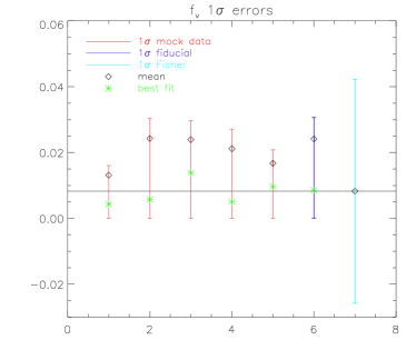
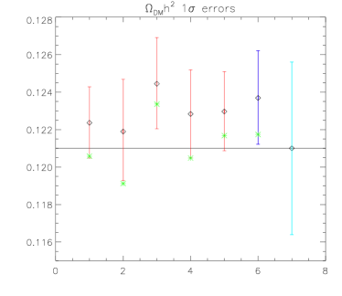
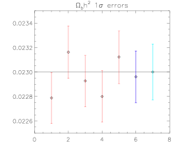
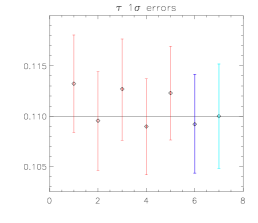
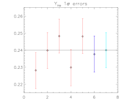
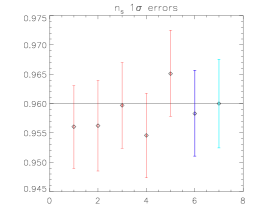
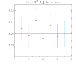
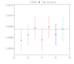
Figures 1 and 2 show the expected sensitivity of Planck to each of the eight parameters. So far, no lensing information (i.e., and ) has been included in the analysis. The errors in these Figures are obtained in three different ways:
-
1.
First, we generate five independent realisations of (see equation (2.6)) from the same cosmological model, the parameter values of which (i.e., ) are indicated by the horizontal lines. The noise power spectrum corresponds to the expected Planck sensitivity (using the three frequency channels with the lowest foreground levels at 100, 143 and 217 GHz, see [21] for details). For each of our five Planck mock data sets, we reconstruct the observed power spectra as per (2.7), sample the likelihood (3.7) with CosmoMC, marginalise over all parameters but one, and plot the mean values and confidence limits (1 errors).
-
2.
Second, we perform the parameter estimation not from a realisation of the fiducial power spectra, but from the fiducial spectra themselves. In other words, we directly sample the likelihood (3.7) with set equal to the theoretical power spectrum of the fiducial model plus the Planck noise spectrum, . This amounts to considering an average over an infinite number of mock Planck data sets. We sample again the likelihood with CosmoMC, marginalise over all parameters but one, and plot the mean values and confidence limits.
- 3.
For all parameters but , the three methods are in good agreement and provide very similar errors . A comparison of the five independent mock data results shows that the errors do not vary significantly from case to case, and that the mean values are nicely distributed around the fiducial value, with a typical dispersion in agreement with the error bars.444Actually, one could object that the error bars are a bit large with respect to the actual scattering of the mean values, particularly for . We attribute this to our crude modelling of the galactic cut (see section 3), which leads to insufficient scattering of the mean values. At this point, the Monte Carlo method based on the fiducial spectrum (method (ii)) and the Fisher matrix approach (method (iii)) both appear to be robust error forecasting techniques.
The conclusions are drastically different for the parameters . The mean values of the five mock data are now distributed asymmetrically with respect to the fiducial values, and the errors predicted by the Fisher matrix are bigger, roughly by a factor two, than those obtained from CosmoMC. Clearly, these problems signal the existence of a non-Gaussian dependence of the likelihood on . A quick way to check this is to plot the best-fit values555Note that, in general, the best-fit values are more efficiently obtained from a minimisation algorithm such as simulated annealing, than from a Monte Carlo method. for each of our CosmoMC runs (green crosses in Figure 2); the best-fit values depart significantly from the mean values, as should be the case for asymmetrical probability distributions. Moreover, the best-fit values are scattered symmetrically around the fiducial values, confirming the fact that the maximum likelihood is an unbiased estimator of . (In contrast, the mean value becomes a biased estimator of as soon as the likelihood departs from Gaussianity with respect to .)
It is easy to understand why the likelihood is non-Gaussian with respect to : is confined to positive values only, cutting the likelihood before it drops to zero. Future experiments or combination of experiments will be confronted to this problem until they have enough sensitivity for making a clear detection of a non-zero neutrino mass.
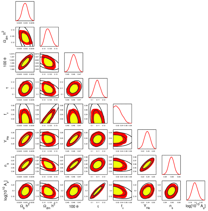
The non-Gaussianity with respect to can be understood from an inspection of Figure 3, which shows the two-dimensional likelihood contours for each pair of parameters (CosmoMC is particularly convenient for obtaining such plots), and the one-dimensional marginalised probabilities on the diagonal. The (1) and (2) confidence contours obtained from the Monte Carlo method (using the fiducial spectra) are shown as the red/yellow (dark/light) filled contours. For all combinations not involving or , remarkable agreement with the black ellipses derived from the Fisher matrix can be seen. (In practice, we obtain the Fisher matrix ellipses by inverting the relevant submatrix, which are then centred on the best-fit parameter values obtained from the Monte Carlo method). From these plots, we see that the parameter is correlated mainly with . This correlation means that any non-Gaussianity in the probability will propagate to . This is why the Fisher matrix ellipses provide a poor approximation of the contours involving and/or .
Better agreement with the Monte Carlo results could perhaps be achieved by adjusting the stepsize when computating the derivatives and for the Fisher matrix. However, as discussed in the section 4, there are no well-controlled methods for doing this unless the full likelihood function is already available.
| method: | MCMC | Fisher | MCMC | Fisher | MCMC | Fisher | MCMC | Fisher |
|---|---|---|---|---|---|---|---|---|
| no lensing | lensing | no lensing | lensing | |||||
| param. | ||||||||
| 0.00022 | 0.00023 | 0.00020 | 0.00021 | 0.00028 | 0.00025 | 0.00023 | 0.00024 | |
| 0.0024 | 0.0046 | 0.0019 | 0.0024 | 0.0092 | 0.0073 | 0.0046 | 0.0048 | |
| 0.016 | 0.034 | 0.008 | 0.011 | 0.030 | 0.040 | 0.009 | 0.013 | |
| 0.0005 | 0.0005 | 0.0004 | 0.0005 | 0.0013 | 0.0011 | 0.0010 | 0.0010 | |
| 0.011 | 0.011 | 0.010 | 0.010 | 0.020 | 0.017 | 0.017 | 0.017 | |
| 0.0048 | 0.0052 | 0.0047 | 0.0047 | 0.0053 | 0.0062 | 0.0050 | 0.0049 | |
| 0.010 | 0.011 | 0.009 | 0.009 | 0.013 | 0.014 | 0.012 | 0.012 | |
| 0.007 | 0.008 | 0.007 | 0.007 | 0.011 | 0.011 | 0.010 | 0.010 | |
| w | - | - | - | - | 0.49 | 0.68 | 0.23 | 0.18 |
| - | - | - | - | 0.46 | 0.27 | 0.27 | 0.26 | |
| - | - | - | - | 0.0090 | 0.0087 | 0.0075 | 0.0077 | |
| (eV) | 0.19 | 0.45 | 0.09 | 0.13 | 0.42 | 0.51 | 0.11 | 0.15 |
| 0.02 | 0.05 | 0.02 | 0.02 | 0.12 | 0.17 | 0.06 | 0.06 | |
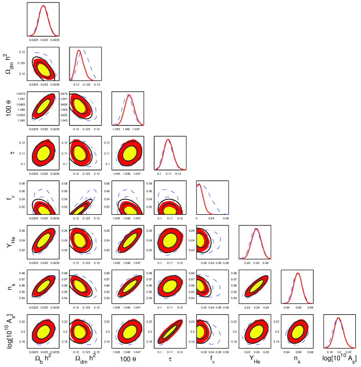
The exercise is repeated in Figure 4, but now with the inclusion of lensing information. Here, we do not generate independent realisations of the data, since the Monte Carlo method utilising the fiducial power spectrum performs equally well for the purpose of error forecasting, as demonstrated in section 5. Lensing extraction is particularly useful for constraining physical quantities that affect the late evolution of cosmological perturbations [34, 12, 14]. These quantities include dark energy (or a cosmological constant) which reduces the growth of matter perturbations at low redshifts, and neutrino masses, which also suppress this growth on small scales.
Since the present parameter basis does not include , the effect of dark energy may be difficult to discern in Figure 4. However, the significant sharpening of the probability distribution is clearly visible. Lensing probes the matter perturbations in a more direct way (than does the CMB alone). This allows for a better determination of through the neutrino’s free-streaming effect on the matter power spectrum. The degeneracy with is also reduced as a consequence. Thus, the likelihood function is now much closer to a multivariate Gaussian, and the Fisher matrix appears to provide satisfactory results, as can be seen from a comparison of the Fisher matrix ellipses with the actual, Monte Carlo contours in Figure 4.
In Table 1, we provide the numerical values of the 1 errors obtained from the Monte Carlo and the Fisher matrix methods, with and without lensing extraction. We show also the corresponding limits for two related parameters, the neutrino mass and the cosmological constant density fraction. Just as for and , the 1 errors for these two quantities are very discrepant between the two cases, since in absence of lensing extraction the Fisher matrix overestimates the error by a factor 2.4, and that on by 2.5.
6 Results including non-minimal parameters
We now study a non-minimal cosmological model with three extra parameters: a (constant) dark energy equation of state , a running spectral index , and the effective number of massless neutrinos (or the number of relativistic fermionic degrees of freedom). Explicitly, our model consists of one massive neutrino responsible for the hot fraction of dark matter , plus a relativistic density attributed to massless neutrinos. Thus, the total number of independent parameters is now eleven.
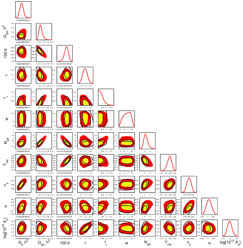
Without lensing extraction, we saw in section 5 that the minimal eight-parameter model was already poorly constrained as a consequence of a mild degeneracy. In the present eleven-parameter model, the situation worsens, mainly because of another parameter degeneracy between , , and (see e.g., [35, 36, 37, 38]). These degeneracies manifest themselves in Figure 5 as very elongated contours, leading clearly to a non-Gaussian likelihood with respect to many cosmological parameters. So, it is not surprising to find that the Fisher matrix is a poor approximation in many cases.
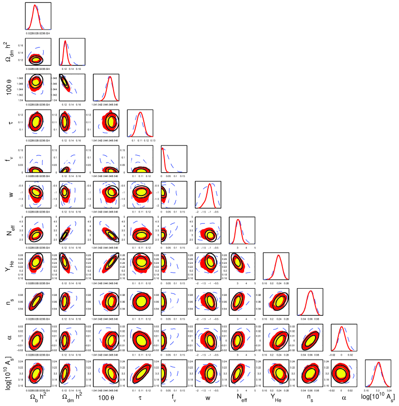
As expected, the inclusion of lensing extraction offers vast improvements in the determination of and . Consequently, the correlations between and and between and essentially disappear (see Figure 6). A reduction of the degeneracy between , and can also be seen, although some correlation between the two parameters remains (since it is possible to vary these parameters simultaneously without changing the epoch of matter–radiation equality). In general, the “lensing” contours in Figure 6 are much more elliptic than their “no lensing” counterparts, indicating that the likelihood is better fitted by a multivariate gaussian.
Table 1 shows the numerical values of the 1 errors for the eleven-parameter model, with and without lensing extraction, obtained from the two forecast methods. In the case without lensing extraction, the Fisher matrix still overestimates the error on and , as well as that on . For , the likelihood is strongly non-gaussian (with large skewness) and the Fisher matrix underestimates the 1 error by a factor 1.7. The discrepancies are even stronger when one looks at the 2 errors.
7 Discussion
We have studied error forecasts on cosmological parameters from the Planck satellite using two different methods. The first is the conventional Fisher matrix analysis in which the second derivative of the parameter likelihood function at the best fit point is used to calculate formal 1 errors on the parameters, as well as the parameter correlation matrix. The second is to use Markov Chain Monte Carlo methods such as CosmoMC on synthetic data sets. This is the same method normally used to extract parameters from present data.
The Monte Carlo method has many advantages over the Fisher matrix approach. While the Fisher matrix uses only information at the best fit point and assumes the likelihood function to be Gaussian with respect to the model parameters, the use of Monte Carlo methods in conjunction with synthetic data maps out the true likelihood function for the given model realisation.
In this paper, we have shown that the likelihood function can be highly non-Gaussian, particularly with respect to the neutrino mass and the dark matter density, and, as a result, the CosmoMC analysis can give results that are very different from its Fisher matrix counterpart. For prospective Planck data without lensing extraction and assuming a simple eight-parameter model, the difference in the projected errors can be as large as a factor of two or more for the said parameters. This indicates that in such cases the Fisher matrix method does not provide a reliable estimation. Including additional data such as CMB lensing information breaks some of the parameter degeneracies, and makes the likelihood more Gaussian. The two methods thus become more compatible.
On the other hand, adding more cosmological parameters (all of which are physically motivated) leads to new parameter degeneracies, and generally worsens the agreement between the two forecast methods. For the eleven-parameter model studied here, we find a difference for the neutrino mass fraction of 45% between the two methods at the 68% level, even with the inclusion of CMB lensing. The conclusion is that for some parameters, even with the very high precision of future data the likelihood function will not be sufficiently Gaussian to yield a reliable estimate of the precision with which the parameter can be measured using the Fisher matrix approach.
Given that Monte Carlo analysis of simulated data sets is computationally feasible with present computers, we propose that future error forecast analyses should employ this method rather than the Fisher matrix analysis. This will have the added advantage that the same parameter extraction pipeline can be used on real data as it becomes available. The present work only includes CMB data simulated to mimic Planck. However, the method can be easily generalised to include other data sets such as future weak lensing and baryon acoustic oscillation surveys.
Acknowledgements
We would like to thank Sergio Pastor and Massimiliano Lattanzi for useful discussions on this work.
References
References
- [1] A. G. Riess et al. [Supernova Search Team Collaboration], Astron. J. 116 (1998) 1009 [arXiv:astro-ph/9805201].
- [2] S. Perlmutter et al. [Supernova Cosmology Project Collaboration], Astrophys. J. 517 (1999) 565 [arXiv:astro-ph/9812133].
- [3] P. Astier et al., Astron. Astrophys. 447 (2006) 31 [arXiv:astro-ph/0510447].
- [4] D. N. Spergel et al. [WMAP Collaboration], Astrophys. J. Suppl. 148 (2003) 175 [arXiv:astro-ph/0302209].
- [5] D. N. Spergel et al., arXiv:astro-ph/0603449.
- [6] M. Tegmark et al. [SDSS Collaboration], Phys. Rev. D 69 (2004) 103501 [arXiv:astro-ph/0310723].
- [7] S. Hannestad, Prog. Part. Nucl. Phys. 57, 309 (2006) [arXiv:astro-ph/0511595].
- [8] J. Lesgourgues and S. Pastor, Phys. Rep. 429, 307 (2006) [arXiv:astro-ph/0603494].
- [9] G. L. Fogli, E. Lisi, A. Marrone, A. Palazzo and A. M. Rotunno, Prog. Part. Nucl. Phys. 57, 71 (2006).
- [10] W. Hu, D.J. Eisenstein and M. Tegmark, Phys. Rev. Lett. 80, 5255 (1998).
- [11] S. Hannestad, Phys. Rev. D 67, 085017 (2003).
- [12] M. Kaplinghat, L. Knox and Y.S. Song, Phys. Rev. Lett. 91, 241301 (2003).
- [13] J. Lesgourgues, S. Pastor and L. Perotto, Phys. Rev. D 70, 045016 (2004) [arXiv:hep-ph/0403296].
- [14] J. Lesgourgues, L. Perotto, S. Pastor and M. Piat, Phys. Rev. D 73, 045021 (2006) [arXiv:astro-ph/0511735].
- [15] S. Hannestad, H. Tu and Y. Y. Y. Wong, arXiv:astro-ph/0603019.
- [16] S. Wang, Z. Haiman, W. Hu, J. Khoury and M. May, Phys. Rev. Lett. 95 (2005) 011302 [arXiv:astro-ph/0505390].
- [17] M. Takada, E. Komatsu and T. Futamase, Phys. Rev. D 73 (2006) 083520 [arXiv:astro-ph/0512374].
- [18] M. Tegmark, A. Taylor and A. Heavens, Astrophys. J. 480, 22 (1997) [arXiv:astro-ph/9603021].
- [19] D.J. Eisenstein, W. Hu and M. Tegmark, Astrophys. J. 518, 2 (1998).
- [20] A. Lewis and S. Bridle, Phys. Rev. D 66, 103511 (2002) [arXiv:astro-ph/0205436].
- [21] Planck Collaboration, arXiv:astro-ph/0604069.
- [22] M. Kamionkowski, A. Kosowsky and A. Stebbins, Phys. Rev. D 55 (1997) 7368 [arXiv:astro-ph/9611125].
- [23] W. T. Hu, arXiv:astro-ph/9508126.
- [24] F. Bernardeau, Astron. Astrophys. 324, 15 (1997).
- [25] M. Zaldarriaga and U. Seljak, Phys. Rev. D 58, 023003 (1998).
- [26] U. Seljak and M. Zaldarriaga, Phys. Rev. Lett. 82, 2636 (1999).
- [27] A. Lewis and A. Challinor, Phys. Rept. 429, 1 (2006) [arXiv:astro-ph/0601594].
- [28] C.M. Hirata and U. Seljak, Phys. Rev. D 68, 083002 (2003).
- [29] T. Okamoto and W. Hu, Phys. Rev. D 67, 083002 (2003).
- [30] W. Hu and T. Okamoto, Astrophys. J. 574, 566 (2002) [arXiv:astro-ph/0111606].
- [31] A. Lewis, A. Challinor and A. Lasenby, Astrophys. J. 538, 473 (2000) [arXiv:astro-ph/9911177].
- [32] B. D. Wandelt, E. Hivon and K. M. Gorski, arXiv:astro-ph/0008111.
- [33] See e.g. M. G. Kendall and A. Stuart, The advanced theory of statistics, 1969.
- [34] W. Hu, Phys. Rev. D 65, 023003 (2002) [arXiv:astro-ph/0108090].
- [35] S. Hannestad, JCAP 0305 (2003) 004 [astro-ph/0303076].
- [36] S. Hannestad and G. Raffelt, JCAP 0404, 008 (2004).
- [37] P. Crotty, J. Lesgourgues and S. Pastor, Phys. Rev. D 69, 123007 (2004) [arXiv:hep-ph/0402049].
- [38] S. Dodelson, A. Melchiorri and A. Slosar, arXiv:astro-ph/0511500.