Galaxy number counts in a presence of the graviton background

Michael A. Ivanov
Physics Dept.,
Belarus State University of Informatics and Radioelectronics,
6 P. Brovka Street, BY 220027, Minsk, Republic of Belarus.
E-mail: ivanovma@gw.bsuir.unibel.by
Abstract

In the model of low-energy quantum gravity by the author, cosmological redshifts are caused by interactions of photons with gravitons. Non-forehead collisions with gravitons will lead to an additional relaxation of any photonic flux. Using only the luminosity distance and a geometrical one as functions of a redshift in this model, theoretical predictions for galaxy number counts are considered here. The Schechter luminosity function with Ξ±=βˆ’2.43𝛼2.43\alpha=-2.43 is used. The considered model provides a good fit to galaxy observations by Yasuda et al. (AJ, 122 (2001) 1104) if the same K-corrections are added. It is shown that observations of N​(z)𝑁𝑧N(z) for different magnitudes mπ‘šm are a lot more informative than the ones of N​(m).π‘π‘šN(m).

1 Introduction

The standard cosmological model explains observations only under the circumstance that almost all matter and energy of the Universe are hidden in some unknown dark forms. In my model of low-energy quantum gravity based on the idea of an existence of the background of super-strong interacting gravitons (for more details, see [1]), a cosmological redshift is caused by interactions of photons with gravitons. Non-forehead collisions with gravitons lead to a very specific additional relaxation of any photonic flux that gives a possibility of another interpretation of supernovae 1a data - without any kinematics or dark energy [1]. I would like to summarize here the main cosmologically essential consequences of this model. Average energy losses of a photon with an energy E𝐸E on a way d​rπ‘‘π‘Ÿdr through the graviton background will be equal to: d​E=βˆ’a​E​d​r,π‘‘πΈπ‘ŽπΈπ‘‘π‘ŸdE=-aEdr, where a=H/c,π‘Žπ»π‘a=H/c, H𝐻H is the Hubble constant. If we introduce a new dimensional constant D𝐷D, so that: σ​(E,Ο΅)=Dβ‹…Eβ‹…Ο΅,𝜎𝐸italic-ϡ⋅𝐷𝐸italic-Ο΅\sigma(E,\epsilon)=D\cdot E\cdot\epsilon, σ​(E,Ο΅)𝜎𝐸italic-Ο΅\sigma(E,\epsilon) is a cross-section of interaction by forehead collisions of a photon with an energy E𝐸E and a graviton with an energy Ο΅,italic-Ο΅\epsilon, then we can compute the Hubble constant in this approach: H=(1/2​π)​D⋅ϡ¯⋅(σ​T4),𝐻⋅12πœ‹π·Β―italic-ϡ𝜎superscript𝑇4H=(1/2\pi)D\cdot\bar{\epsilon}\cdot(\sigma T^{4}), where ϡ¯¯italic-Ο΅\bar{\epsilon} is an average graviton energy, and T𝑇T is a temperature of the background. The constant D𝐷D should have the value: D=0.795β‹…10βˆ’27​m2/e​V2;𝐷⋅0.795superscript1027superscriptπ‘š2𝑒superscript𝑉2D=0.795\cdot 10^{-27}{m^{2}/eV^{2}}; the one may be found from the Newtonian limit of gravity. If rπ‘Ÿr is a geometrical distance from a source, then we have for r​(z)π‘Ÿπ‘§r(z), z𝑧z is a redshift: r​(z)=l​n​(1+z)/a.π‘Ÿπ‘§π‘™π‘›1π‘§π‘Žr(z)=ln(1+z)/a. None-forehead collisions of photons with gravitons of the background will lead to a scatter of photons and to an additional relaxation of a photonic flux, so that the luminosity distance DLsubscript𝐷𝐿D_{L} is equal in this approach to: DL=aβˆ’1​ln⁑(1+z)β‹…(1+z)(1+b)/2≑aβˆ’1​f1​(z),subscript𝐷𝐿⋅superscriptπ‘Ž11𝑧superscript1𝑧1𝑏2superscriptπ‘Ž1subscript𝑓1𝑧D_{L}=a^{-1}\ln(1+z)\cdot(1+z)^{(1+b)/2}\equiv a^{-1}f_{1}(z), where f1​(z)≑ln⁑(1+z)β‹…(1+z)(1+b)/2subscript𝑓1𝑧⋅1𝑧superscript1𝑧1𝑏2f_{1}(z)\equiv\ln(1+z)\cdot(1+z)^{(1+b)/2} is the luminosity distance in units of c/H.𝑐𝐻c/H. This luminosity distance function fits supernova observations very well for roughly z<0.5𝑧0.5z<0.5. It excludes a need of any dark energy to explain supernovae dimming.

In this paper, I consider galaxy number counts/redshift and counts/magnitude relations on a basis of this model. I assume here that a space is flat and the Universe is not expanding.

2 The galaxy number counts-redshift relation

Total galaxy number counts d​N​(r)π‘‘π‘π‘ŸdN(r) for a volume element d​V=d​Ω​r2​d​r𝑑𝑉𝑑Ωsuperscriptπ‘Ÿ2π‘‘π‘ŸdV=d\Omega r^{2}dr is equal to: d​N​(r)=ng​d​V=ng​d​Ω​r2​d​r,π‘‘π‘π‘Ÿsubscript𝑛𝑔𝑑𝑉subscript𝑛𝑔𝑑Ωsuperscriptπ‘Ÿ2π‘‘π‘ŸdN(r)=n_{g}dV=n_{g}d\Omega r^{2}dr, where ngsubscript𝑛𝑔n_{g} is a galaxy number density (it is constant in the no-evolution scenario), d​Ω𝑑Ωd\Omega is a solid angle element. Using the function r​(z)π‘Ÿπ‘§r(z) of this model, we can re-write galaxy number counts as a function of a redshift z𝑧z:

d​N​(z)=ng​d​Ω​(H/c)βˆ’3​l​n2​(1+z)1+z​d​z.𝑑𝑁𝑧subscript𝑛𝑔𝑑Ωsuperscript𝐻𝑐3𝑙superscript𝑛21𝑧1𝑧𝑑𝑧dN(z)=n_{g}d\Omega(H/c)^{-3}{ln^{2}(1+z)\over{1+z}}dz. (1)

Let us introduce a function (see [2])

f2​(z)≑(H/c)3​d​N​(z)ng​d​Ω​z2​d​z;subscript𝑓2𝑧superscript𝐻𝑐3𝑑𝑁𝑧subscript𝑛𝑔𝑑Ωsuperscript𝑧2𝑑𝑧f_{2}(z)\equiv{(H/c)^{3}dN(z)\over n_{g}d\Omega z^{2}dz};

then we have for it in this model:

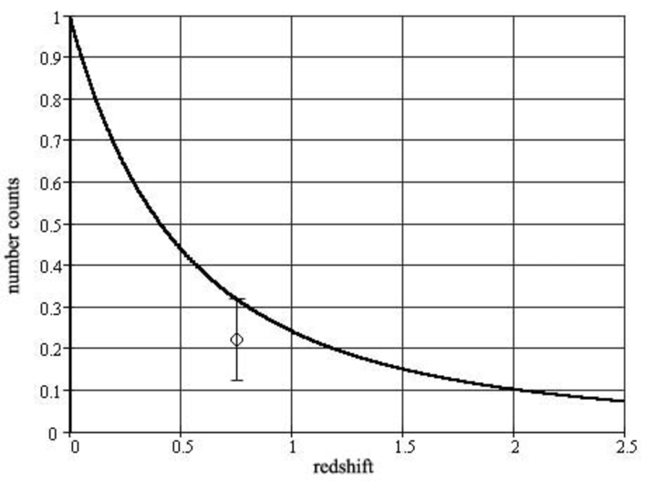
f2​(z)=l​n2​(1+z)z2​(1+z).subscript𝑓2𝑧𝑙superscript𝑛21𝑧superscript𝑧21𝑧f_{2}(z)={ln^{2}(1+z)\over{z^{2}(1+z)}}. (2)

A graph of this function is shown in Fig. 1; the typical error bar and data point are added here from paper [3] by Loh and Spillar. There is not a visible contradiction with observations. There is not any free parameter in the model to fit this curve; it is a very rigid case.
Refer to caption

Figure 1: Number counts f2subscript𝑓2f_{2} as a function of the redshift in this model. The typical error bar and data point are taken from paper [3] by Loh and Spillar.

It is impossible to count a total galaxy number for big redshifts so as very faint galaxies are not observable. For objects with a fixed luminosity, it is easy to find how their magnitude mπ‘šm changes with a redshift. So as d​m​(z)π‘‘π‘šπ‘§dm(z) under a constant luminosity is equal to: d​m​(z)=5​d​(l​g​DL​(z)),π‘‘π‘šπ‘§5𝑑𝑙𝑔subscript𝐷𝐿𝑧dm(z)=5d(lgD_{L}(z)), we have for Δ​m​(z1,z2)β‰‘βˆ«z1z2𝑑m​(z)::Ξ”π‘šsubscript𝑧1subscript𝑧2superscriptsubscriptsubscript𝑧1subscript𝑧2differential-dπ‘šπ‘§absent\Delta m(z_{1},z_{2})\equiv\int_{z_{1}}^{z_{2}}dm(z):

Δ​m​(z1,z2)=5​l​g​(f1​(z2)/f1​(z1)).Ξ”π‘šsubscript𝑧1subscript𝑧25𝑙𝑔subscript𝑓1subscript𝑧2subscript𝑓1subscript𝑧1\Delta m(z_{1},z_{2})=5lg(f_{1}(z_{2})/f_{1}(z_{1})). (3)

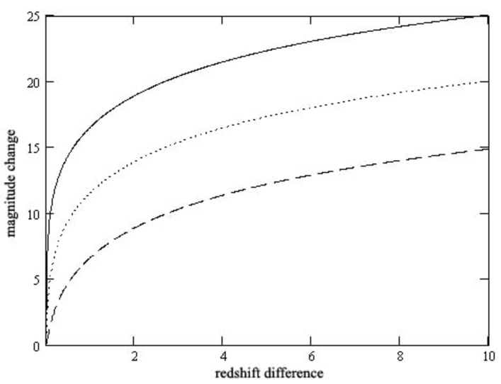
This function is shown in Fig.2 for z1=0.001;0.01;0.1.subscript𝑧10.0010.010.1z_{1}=0.001;0.01;0.1.

Refer to caption

Figure 2: Magnitude changes Δ​mΞ”π‘š\Delta m as a function of the redshift difference z2βˆ’z1subscript𝑧2subscript𝑧1z_{2}-z_{1} in this model for z1=0.001subscript𝑧10.001z_{1}=0.001 (solid); 0.01 (dot); 0.1 (dash).

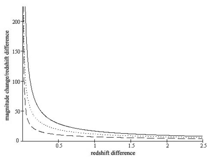
I would like to note that a very fast initial growth of the luminosity distance with a redshift z𝑧z in this model might explain the observed excess of faint blue galaxy number counts above an expected one in the standard model (for example, see [4]). A galaxy color depends on a redshift, and a galaxy dimming depends on the luminosity distance, because by big values of the ratio Δ​m​(z1,z2)/(z2βˆ’z1)Ξ”π‘šsubscript𝑧1subscript𝑧2subscript𝑧2subscript𝑧1\Delta m(z_{1},z_{2})/(z_{2}-z_{1}) in a region of small redshifts and by a further much slower change of it (see Fig.3) an observer will see many faint but blue enough galaxies in this region (in the no-evolution scenario).
Refer to caption

Figure 3: To a possible explanation of the excess of faint blue galaxy number counts: Δ​m​(z1,z2)/(z2βˆ’z1)Ξ”π‘šsubscript𝑧1subscript𝑧2subscript𝑧2subscript𝑧1\Delta m(z_{1},z_{2})/(z_{2}-z_{1}) vs. the redshift difference z2βˆ’z1subscript𝑧2subscript𝑧1z_{2}-z_{1} in this model for z1=0.001subscript𝑧10.001z_{1}=0.001 (solid); 0.01 (dot); 0.1 (dash).

3 Taking into account the galaxy luminosity function

Galaxies have different luminosities L,𝐿L, and we can write ngsubscript𝑛𝑔n_{g} as an integral: ng=βˆ«π‘‘ng​(L),subscript𝑛𝑔differential-dsubscript𝑛𝑔𝐿n_{g}=\int dn_{g}(L), where d​ng​(L)=η​(L)​d​L,𝑑subscriptπ‘›π‘”πΏπœ‚πΏπ‘‘πΏdn_{g}(L)=\eta(L)dL, η​(L)πœ‚πΏ\eta(L) is the galaxy luminosity function. I shall use here the Schechter luminosity function [5]:

η​(L)​d​L=Ο•βˆ—β€‹(LLβˆ—)α​e​x​p​(βˆ’LLβˆ—)​d​(LLβˆ—)πœ‚πΏπ‘‘πΏsubscriptitalic-Ο•βˆ—superscript𝐿subscriptπΏβˆ—π›Όπ‘’π‘₯𝑝𝐿subscriptπΏβˆ—π‘‘πΏsubscriptπΏβˆ—\eta(L)dL=\phi_{\ast}({L\over L_{\ast}})^{\alpha}exp(-{L\over L_{\ast}})d({L\over L_{\ast}}) (4)

with the parameters Ο•βˆ—,subscriptitalic-Ο•βˆ—\phi_{\ast}, Lβˆ—,subscriptπΏβˆ—L_{\ast}, Ξ±.𝛼\alpha.111To turn aside the problem with divergencies of this function by small L𝐿L for negative values of Ξ±,𝛼\alpha, all computations are performed here for z>0.001.𝑧0.001z>0.001. So as we have by a definition of the luminosity distance DL​(z)subscript𝐷𝐿𝑧D_{L}(z) that a light flux I𝐼I is equal to: I=L4​π​DL2​(z),𝐼𝐿4πœ‹superscriptsubscript𝐷𝐿2𝑧I={L\over 4\pi D_{L}^{2}(z)}, and a visible magnitude mπ‘šm of an object is m=βˆ’2.5​lg⁑I+C,π‘š2.5lg𝐼𝐢m=-2.5\lg I+C, where C𝐢C is a constant, then mπ‘šm is equal to:

m=βˆ’2.5​lg⁑I+5​lg⁑DL​(z)+(Cβˆ’4​π).π‘š2.5lg𝐼5lgsubscript𝐷𝐿𝑧𝐢4πœ‹m=-2.5\lg I+5\lg D_{L}(z)+(C-4\pi). (5)

We can write for L::𝐿absentL:

L=Aβ‹…DL2​(z)ΞΊm,𝐿⋅𝐴superscriptsubscript𝐷𝐿2𝑧superscriptπœ…π‘šL=A\cdot{D_{L}^{2}(z)\over\kappa^{m}}, (6)

where ΞΊ=100.4,A=c​o​n​s​t.formulae-sequenceπœ…superscript100.4π΄π‘π‘œπ‘›π‘ π‘‘\kappa=10^{0.4},\ A=const. For a thin layer with z=c​o​n​s​tπ‘§π‘π‘œπ‘›π‘ π‘‘z=const we have:

d​L=βˆ‚Lβˆ‚mβ‹…d​m,π‘‘πΏβ‹…πΏπ‘šπ‘‘π‘šdL={\partial L\over\partial m}\cdot dm,

where

βˆ‚Lβˆ‚m=βˆ’m​κ⋅A​DL2​(z)ΞΊm=βˆ’m​κ​L.πΏπ‘šβ‹…π‘šπœ…π΄superscriptsubscript𝐷𝐿2𝑧superscriptπœ…π‘šπ‘šπœ…πΏ{\partial L\over\partial m}=-m\kappa\cdot A{D_{L}^{2}(z)\over\kappa^{m}}=-m\kappa L. (7)

Then

d​ng​(m,z)=βˆ’(Ο•βˆ—β€‹ΞΊ)β‹…lα​(m,z)​exp⁑(βˆ’l​(m,z))β‹…(mβ‹…l​(m,z))​d​m,𝑑subscriptπ‘›π‘”π‘šπ‘§β‹…β‹…subscriptitalic-Ο•βˆ—πœ…superscriptπ‘™π›Όπ‘šπ‘§π‘™π‘šπ‘§β‹…π‘šπ‘™π‘šπ‘§π‘‘π‘šdn_{g}(m,z)=-(\phi_{\ast}\kappa)\cdot l^{\alpha}(m,z)\exp(-l(m,z))\cdot(m\cdot l(m,z))dm, (8)

where (βˆ’d​m)π‘‘π‘š(-dm) corresponds to decreasing mπ‘šm by growing L𝐿L when z=c​o​n​s​t,π‘§π‘π‘œπ‘›π‘ π‘‘z=const, and

l​(m,z)≑L​(m,z)Lβˆ—.π‘™π‘šπ‘§πΏπ‘šπ‘§subscriptπΏβˆ—l(m,z)\equiv{L(m,z)\over L_{\ast}}.

Let us introduce a function f3​(m,z)subscript𝑓3π‘šπ‘§f_{3}(m,z) with a differential

d​f3​(m,z)≑d​N​(m,z)dΞ©(βˆ’dm).df_{3}(m,z)\equiv{dN(m,z)\over d\Omega(-dm).} (9)

We have for this differential in the model:

d​f3​(m,z)=(Ο•βˆ—β€‹ΞΊa3)β‹…mβ‹…lΞ±+1​(m,z)β‹…exp⁑(βˆ’l​(m,z))β‹…l​n2​(1+z)(1+z)​d​z,𝑑subscript𝑓3π‘šπ‘§β‹…β‹…subscriptitalic-Ο•βˆ—πœ…superscriptπ‘Ž3π‘šsuperscript𝑙𝛼1π‘šπ‘§π‘™π‘šπ‘§π‘™superscript𝑛21𝑧1𝑧𝑑𝑧df_{3}(m,z)=({\phi_{\ast}\kappa\over a^{3}})\cdot m\cdot l^{\alpha+1}(m,z)\cdot\exp(-l(m,z))\cdot{ln^{2}(1+z)\over(1+z)}dz, (10)

where a=H/cπ‘Žπ»π‘a=H/c, H𝐻H is the Hubble constant. An integral on z𝑧z gives the galaxy number counts/magnitude relation:

f3​(m)=(Ο•βˆ—β€‹ΞΊa3)β‹…mβ‹…βˆ«0zm​a​xlΞ±+1​(m,z)β‹…exp⁑(βˆ’l​(m,z))β‹…l​n2​(1+z)(1+z)​𝑑z;subscript𝑓3π‘šβ‹…subscriptitalic-Ο•βˆ—πœ…superscriptπ‘Ž3π‘šsuperscriptsubscript0subscriptπ‘§π‘šπ‘Žπ‘₯β‹…superscript𝑙𝛼1π‘šπ‘§π‘™π‘šπ‘§π‘™superscript𝑛21𝑧1𝑧differential-d𝑧f_{3}(m)=({\phi_{\ast}\kappa\over a^{3}})\cdot m\cdot\int_{0}^{z_{max}}l^{\alpha+1}(m,z)\cdot\exp(-l(m,z))\cdot{ln^{2}(1+z)\over(1+z)}dz; (11)

I use here an upper limit zm​a​x=10.subscriptπ‘§π‘šπ‘Žπ‘₯10z_{max}=10. To compare this function with observations by Yasuda et al. [6], let us choose the normalizing factor from the condition: f3​(16)=a​(16),subscript𝑓316π‘Ž16f_{3}(16)=a(16), where

a​(m)≑AΞ»β‹…100.6​(mβˆ’16)π‘Žπ‘šβ‹…subscriptπ΄πœ†superscript100.6π‘š16a(m)\equiv A_{\lambda}\cdot 10^{0.6(m-16)} (12)

is the function assuming ”Euclidean” geometry and giving the best fit to observations [6], AΞ»=c​o​n​s​tsubscriptπ΄πœ†π‘π‘œπ‘›π‘ π‘‘A_{\lambda}=const depends on the spectral band. In this case, we have two free parameters - α𝛼\alpha and Lβˆ—subscriptπΏβˆ—L_{\ast} - to fit observations, and the latter one is connected with a constant A1≑Aa2​Lβˆ—subscript𝐴1𝐴superscriptπ‘Ž2subscriptπΏβˆ—A_{1}\equiv{A\over a^{2}L_{\ast}} if

l​(m,z)=A1​f12​(z)ΞΊm.π‘™π‘šπ‘§subscript𝐴1superscriptsubscript𝑓12𝑧superscriptπœ…π‘šl(m,z)=A_{1}{f_{1}^{2}(z)\over\kappa^{m}}.

If we use the magnitude scale in which m=0π‘š0m=0 for Vega then C=2.5​lg⁑IV​e​g​a,𝐢2.5lgsubscriptπΌπ‘‰π‘’π‘”π‘ŽC=2.5\lg I_{Vega}, and we get for A1subscript𝐴1A_{1} by H=2.14β‹…10βˆ’18​sβˆ’1𝐻⋅2.14superscript1018superscript𝑠1H=2.14\cdot 10^{-18}\ s^{-1} (it is a theoretical estimate of H𝐻H in this model [1]):

A1≃5β‹…1017β‹…LβŠ™Lβˆ—,similar-to-or-equalssubscript𝐴1β‹…5superscript1017subscript𝐿direct-productsubscriptπΏβˆ—A_{1}\simeq 5\cdot 10^{17}\cdot{L_{\odot}\over L_{\ast}}, (13)

where LβŠ™subscript𝐿direct-productL_{\odot} is the Sun luminosity; the following values are used: LV​e​g​a=50​LβŠ™,subscriptπΏπ‘‰π‘’π‘”π‘Ž50subscript𝐿direct-productL_{Vega}=50L_{\odot}, the distance to Vega rV​e​g​a=26​L​Y.subscriptπ‘Ÿπ‘‰π‘’π‘”π‘Ž26πΏπ‘Œr_{Vega}=26\ LY.

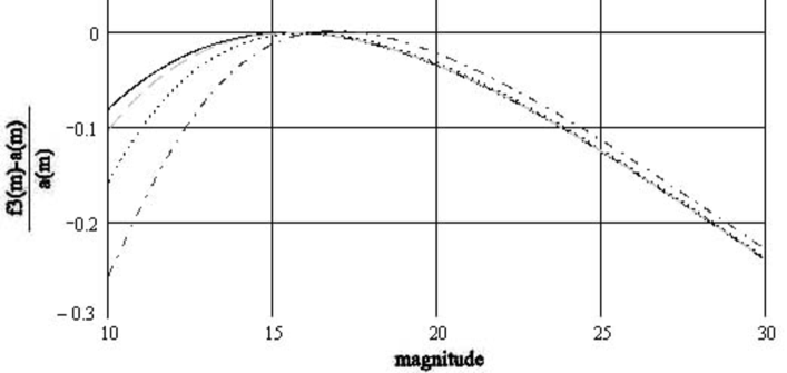
Without the factor m,π‘šm, the function f3​(m)subscript𝑓3π‘šf_{3}(m) by exp(βˆ’l(m,z)β†’1\exp(-l(m,z)\rightarrow 1 would be close to a​(m)π‘Žπ‘ša(m) by Ξ±=βˆ’2.5.𝛼2.5\alpha=-2.5. Matching values of α𝛼\alpha shows that f3​(m)subscript𝑓3π‘šf_{3}(m) is the closest to a​(m)π‘Žπ‘ša(m) in the range 10<m<2010π‘š2010<m<20 by Ξ±=βˆ’2.43.𝛼2.43\alpha=-2.43. The ratio f3​(m)βˆ’a​(m)a​(m)subscript𝑓3π‘šπ‘Žπ‘šπ‘Žπ‘š{{f_{3}(m)-a(m)}\over a(m)} is shown in Fig.4 for different values of A1subscript𝐴1A_{1} by this value of α𝛼\alpha. All such the curves conflow by

Refer to caption

Figure 4: The relative difference (f3​(m)βˆ’a​(m))/a​(m)subscript𝑓3π‘šπ‘Žπ‘šπ‘Žπ‘š(f_{3}(m)-a(m))/a(m) as a function of the magnitude mπ‘šm for Ξ±=βˆ’2.43𝛼2.43\alpha=-2.43 by 10βˆ’2<A1<102superscript102subscript𝐴1superscript10210^{-2}<A_{1}<10^{2} (solid), A1=104subscript𝐴1superscript104A_{1}=10^{4} (dash), A1=105subscript𝐴1superscript105A_{1}=10^{5} (dot), A1=106subscript𝐴1superscript106A_{1}=10^{6} (dadot).

A1≀102subscript𝐴1superscript102A_{1}\leq 10^{2} (or 5β‹…1015<Lβˆ—β‹…5superscript1015subscriptπΏβˆ—5\cdot 10^{15}<L_{\ast}), i.e. observations of the galaxy number counts/magnitude relation are non-sensitive to A1subscript𝐴1A_{1} in this range. For fainter magnitudes 20<m<3020π‘š3020<m<30, the behavior of all curves is identical: they go below of the ratio value 111 with the same slope. If we compare this figure with Figs. 6,10,12 from [6], we see that the considered model provides a no-worse fit to observations than the function a​(m)π‘Žπ‘ša(m) if the same K-corrections are added (I think that even a better one if one takes into account positions of observational points in Figs. 6,10,12 from [6] by m<16π‘š16m<16 and m>16π‘š16m>16) for the range 102<A1<107superscript102subscript𝐴1superscript10710^{2}<A_{1}<10^{7} that corresponds to 5β‹…1015>Lβˆ—>5β‹…1010.β‹…5superscript1015subscriptπΏβˆ—β‹…5superscript10105\cdot 10^{15}>L_{\ast}>5\cdot 10^{10}.

Observations of N​(z)𝑁𝑧N(z) for different magnitudes are a lot more informative. If we define a function f4​(m,z)subscript𝑓4π‘šπ‘§f_{4}(m,z) as

f4​(m,z)≑(a3Ο•βˆ—β€‹ΞΊ)β‹…d​f3​(m,z)d​z,subscript𝑓4π‘šπ‘§β‹…superscriptπ‘Ž3subscriptitalic-Ο•βˆ—πœ…π‘‘subscript𝑓3π‘šπ‘§π‘‘π‘§f_{4}(m,z)\equiv({a^{3}\over\phi_{\ast}\kappa})\cdot{df_{3}(m,z)\over dz}, (14)

this function is equal in the model to:

f4​(m,z)=mβ‹…lΞ±+1​(m,z)β‹…exp⁑(βˆ’l​(m,z))β‹…l​n2​(1+z)(1+z).subscript𝑓4π‘šπ‘§β‹…β‹…π‘šsuperscript𝑙𝛼1π‘šπ‘§π‘™π‘šπ‘§π‘™superscript𝑛21𝑧1𝑧f_{4}(m,z)=m\cdot l^{\alpha+1}(m,z)\cdot\exp(-l(m,z))\cdot{ln^{2}(1+z)\over(1+z)}. (15)

Galaxy number counts in the range m1<m<m2subscriptπ‘š1π‘šsubscriptπ‘š2m_{1}<m<m_{2} are proportional to the function:

f5​(m1,m2)β‰‘βˆ«m1m2f4​(m,z)​𝑑m=subscript𝑓5subscriptπ‘š1subscriptπ‘š2superscriptsubscriptsubscriptπ‘š1subscriptπ‘š2subscript𝑓4π‘šπ‘§differential-dπ‘šabsentf_{5}(m_{1},m_{2})\equiv\int_{m_{1}}^{m_{2}}f_{4}(m,z)dm= (16)
=∫m1m2mβ‹…lΞ±+1​(m,z)β‹…exp⁑(βˆ’l​(m,z))β‹…l​n2​(1+z)(1+z)​𝑑m.absentsuperscriptsubscriptsubscriptπ‘š1subscriptπ‘š2β‹…β‹…π‘šsuperscript𝑙𝛼1π‘šπ‘§π‘™π‘šπ‘§π‘™superscript𝑛21𝑧1𝑧differential-dπ‘š=\int_{m_{1}}^{m_{2}}m\cdot l^{\alpha+1}(m,z)\cdot\exp(-l(m,z))\cdot{ln^{2}(1+z)\over(1+z)}dm.

Refer to caption

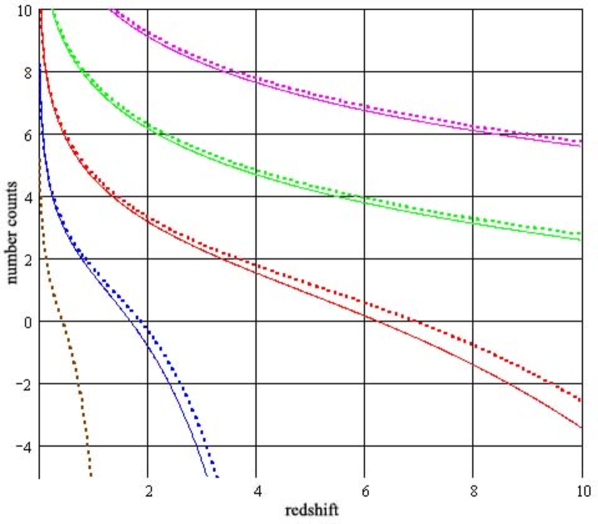
Figure 5: Number counts f4​(m,z)subscript𝑓4π‘šπ‘§f_{4}(m,z) (dot) and f5​(m1,m2)subscript𝑓5subscriptπ‘š1subscriptπ‘š2f_{5}(m_{1},m_{2}) (solid) (logarithmic scale) as a function of the redshift by A1=105subscript𝐴1superscript105A_{1}=10^{5} for Ξ±=βˆ’2.43,m1=10formulae-sequence𝛼2.43subscriptπ‘š110\alpha=-2.43,\ m_{1}=10 and different values of m=m2::π‘šsubscriptπ‘š2absentm=m_{2}: 15 (blue), 20 (red), 25 (green), and 30 (mag); m=10π‘š10m=10 (brown, only f4​(m,z)subscript𝑓4π‘šπ‘§f_{4}(m,z)),.

Graphs of both f4​(m,z)subscript𝑓4π‘šπ‘§f_{4}(m,z) and f5​(m1,m2)subscript𝑓5subscriptπ‘š1subscriptπ‘š2f_{5}(m_{1},m_{2}) are shown in Fig. 5 by Ξ±=βˆ’2.43,A1=105formulae-sequence𝛼2.43subscript𝐴1superscript105\alpha=-2.43,\ A_{1}=10^{5}; they are very similar between themselves. We see that even the observational fact that a number of visible galaxies by z∼10similar-to𝑧10z\sim 10 is very small allows us to restrict a value of the parameter A1subscript𝐴1A_{1} much stronger than observations of N​(m)π‘π‘šN(m).

4 Quasar number counts

For quasars, we can attempt to compute the galaxy number counts/redshift relation using Eq. 16 with another luminosity function Ξ·(l(m,z))β€²\eta{{}^{\prime}}(l(m,z)):

f5(m1,m2)β‰‘βˆ«m1m2f4(m,z)β€²dm=∫m1m2mβ‹…l(m,z)β‹…Ξ·(l(m,z))β€²β‹…l​n2​(1+z)(1+z)dz.f_{5}(m_{1},m_{2})\equiv\int_{m_{1}}^{m_{2}}f_{4}{{}^{\prime}}(m,z)dm=\int_{m_{1}}^{m_{2}}m\cdot l(m,z)\cdot\eta{{}^{\prime}}(l(m,z))\cdot{ln^{2}(1+z)\over(1+z)}dz. (17)

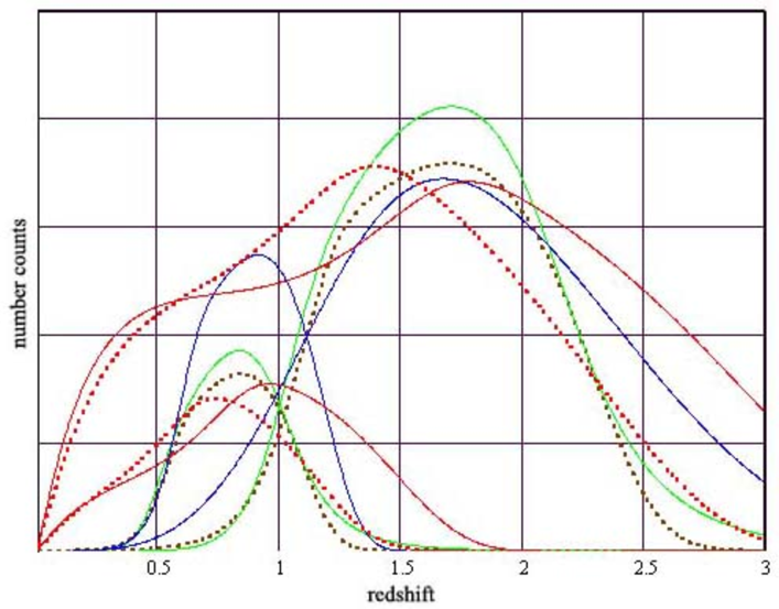
The following luminosity functions were probed here (see Fig. 6): the Schechter one with Ξ±=0𝛼0\alpha=0, A1=106.55subscript𝐴1superscript106.55A_{1}=10^{6.55} (blue); the double power law [7, 8]:

Ξ·(l(m,z))β€²βˆ1lβˆ’Ξ±β€‹(m,z)+lβˆ’Ξ²β€‹(m,z)\eta{{}^{\prime}}(l(m,z))\propto{1\over l^{-\alpha}(m,z)+l^{-\beta}(m,z)} (18)

with Ξ±=βˆ’3.9,Ξ²=1.6,A1=4.5β‹…106formulae-sequence𝛼3.9formulae-sequence𝛽1.6subscript𝐴1β‹…4.5superscript106\alpha=-3.9,\ \beta=1.6,\ A_{1}=4.5\cdot 10^{6} (green); the Gaussian one:

Ξ·(l(m,z))β€²βˆexp(βˆ’(l​(m,z)βˆ’1)22​σ2)\eta{{}^{\prime}}(l(m,z))\propto\exp({-(l(m,z)-1)^{2}\over 2\sigma^{2}}) (19)

with Οƒ=0.5,A1=4.5β‹…106formulae-sequence𝜎0.5subscript𝐴1β‹…4.5superscript106\sigma=0.5,\ A_{1}=4.5\cdot 10^{6} (brown, dot); the combined one:

Ξ·(l(m,z))β€²βˆlΞ±(m,z)β‹…exp(βˆ’(l​(m,z)βˆ’1)22​σ2)\eta{{}^{\prime}}(l(m,z))\propto l^{\alpha}(m,z)\cdot\exp({-(l(m,z)-1)^{2}\over 2\sigma^{2}}) (20)

with two sets of parameters: Ξ±=βˆ’1.45,Οƒ=0.6,A1=1.3β‹…106formulae-sequence𝛼1.45formulae-sequence𝜎0.6subscript𝐴1β‹…1.3superscript106\alpha=-1.45,\ \sigma=0.6,\ A_{1}=1.3\cdot 10^{6} (red, solid) and Ξ±=βˆ’1.4,Οƒ=0.7,A1=3β‹…106formulae-sequence𝛼1.4formulae-sequence𝜎0.7subscript𝐴1β‹…3superscript106\alpha=-1.4,\ \sigma=0.7,\ A_{1}=3\cdot 10^{6} (red, dot). There is a couple of

Refer to caption

Figure 6: QSO number counts f5​(m,z)subscript𝑓5π‘šπ‘§f_{5}(m,z) (arbitrary units) as a function of the redshift for different luminosity functions: Gaussian (brown, dot), the double power law (green), Schechter’s (blue), combined (red, solid and dot) with parameters given in the text. The left-shifted curve of each couple corresponds to the range 16<m<18.25,16π‘š18.2516<m<18.25, another one corresponds to 18.25<m<20.85.18.25π‘š20.8518.25<m<20.85.

curves for each case: the left-shifted curve of any couple corresponds to the range 16<m<18.25,16π‘š18.2516<m<18.25, another one corresponds to 18.25<m<20.85.18.25π‘š20.8518.25<m<20.85. These ranges are chosen the same as in the paper by Croom et al. [7], and you may compare this figure with Fig. 3 in [7]. We can see that the theoretical distributions reflect only some features of the observed ones but not an entire picture. In all these cases, a slope of an analog of log⁑(f3​(m))subscript𝑓3π‘š\log(f_{3}(m)) near m=18π‘š18m=18 is in the range 0.29 - 0.325, when quasar observations give a larger slope (see Fig. 4, 21 in [7] and Fig. 13 in [9]; in the latter paper, this slope has been evaluated to be equal to about 1). We can summarize that, as well as in the standard cosmological model, it is impossible to fit quasar observations using some simple luminosity function with fixed parameters.

In the standard model, an easy way exists to turn aside this difficulty: one ascribes it to a quasar ”evolution”, then a luminosity function (for example, the double power law [7, 8]) is modified for different redshifts to take into account this ”evolution”. There exist two manner to do it: one may consider Lβˆ—subscriptπΏβˆ—L_{\ast} as a function of a redshift (pure luminosity evolution) [7] or one may assume that indices α𝛼\alpha and β𝛽\beta of the distribution (double power law) vary with z𝑧z [8] - in both variants, it is possible to fit observations in some range of redshifts; of course, there are many other descriptions of the ”evolution” [9]. It is strange only that ”evolutions” are not concerted: we can see exponential, quadratic and other kinds of them - and it means that there is not any real evolution: we deal with a pure fine art of fitting, nothing more. In the considered model, this way is forbidden.

I think that it is necessary to consider some theoretical model of a quasar activity to get a distribution of ”instantaneous” luminosities. It is known that the typical lifetime of individual quasars is uncertain by several orders of magnitude; a lifetime of 4β‹…107β‹…4superscript1074\cdot 10^{7} years may be considered as an average value [10]. If one considers a quasar light curve L​(t)𝐿𝑑L(t) (in a manner which is similar to the one by Hopkins et al. [11]) in a parametric form, it is possible to get the luminosity function which takes into account a probability to observe a quasar with a given luminosity. Let us consider the two simple examples. The simplest case is a constant luminosity L𝐿L of any quasar during its lifetime Ο„πœ\tau. If initial moments of quasar activity are distributed uniformly in time and may be described by a frequency ν𝜈\nu, then a probability Po​b​ssubscriptπ‘ƒπ‘œπ‘π‘ P_{obs} to observe a quasar will be equal to:

Po​b​s=∫0Ο„exp(βˆ’Ξ½t)β€²d(Ξ½t)β€²=1βˆ’exp(βˆ’Ξ½Ο„).P_{obs}=\int_{0}^{\tau}\exp(-\nu t{{}^{\prime}})d(\nu t{{}^{\prime}})=1-\exp(-\nu\tau). (21)

For ν​τβ‰ͺ1much-less-than𝜈𝜏1\nu\tau\ll 1 we have Po​b​s≃ν​τ.similar-to-or-equalssubscriptπ‘ƒπ‘œπ‘π‘ πœˆπœP_{obs}\simeq\nu\tau. If we further assume that Ο„βˆ1/L,proportional-to𝜏1𝐿\tau\propto 1/L, i.e. that a full emitted quasar energy is constant, then a distribution of observable luminosities is

Ξ·(L)β€²βˆΞ·(L)β‹…1/L,\eta{{}^{\prime}}(L)\propto\eta(L)\cdot 1/L, (22)

where η​(L)πœ‚πΏ\eta(L) is an initial distribution of values of L𝐿L.

The second example is the quasar exponential light curve:

L​(t)=L0​exp⁑(βˆ’t/Ο„),𝐿𝑑subscript𝐿0π‘‘πœL(t)=L_{0}\exp(-t/\tau), (23)

where Ο„πœ\tau is a lifetime, L0subscript𝐿0L_{0} is an initial luminosity. If L0subscript𝐿0L_{0} has a distribution η​(L0)πœ‚subscript𝐿0\eta(L_{0}), then we get:

Ξ·(L)β€²βˆβˆ«Ξ·(L0)β‹…[exp(tm​a​x/Ο„(L0))βˆ’1]βˆ’1β‹…(L0/L)2βˆ’Ξ½β€‹Ο„β€‹(L0)β‹…dL0,\eta{{}^{\prime}}(L)\propto\int\eta(L_{0})\cdot[\exp(t_{max}/\tau(L_{0}))-1]^{-1}\cdot(L_{0}/L)^{2-\nu\tau(L_{0})}\cdot dL_{0}, (24)

where tm​a​xsubscriptπ‘‘π‘šπ‘Žπ‘₯t_{max} is a maximum time during which one can distinguish a quasar from a host galaxy, and Ο„πœ\tau depends on L0subscript𝐿0L_{0} in some manner. We see that even in this simple toy example the dependence on Ο„πœ\tau is not trivial.

In a general case, it is necessary to describe both - front and back - slopes of a quasar light curve. Together with a total emitted energy (or a peak luminosity), we need at least three independent parameters; if we take into account their random distributions, this number should be at least doubled.

5 Conclusion

Starting from a micro level and considering interactions of photons with single gravitons, we can find the luminosity distance and a geometrical distance in this approach. Using only these quantities, I compute here galaxy number counts-redshift and galaxy number counts-magnitude relations for a case of a flat non-expanding universe. It has been shown here that they are in a good accordance with observations. It may be important as for cosmology as for a theory of gravity.

References

  • [1] Ivanov, M.A. Gravitons as super-strong interacting particles, and low-energy quantum gravity. In the book Focus on Quantum Gravity Research, Nova Science, 2006, Chapter 3 (in press); [hep-th/0506189 v3]; [http://ivanovma.narod.ru/nova04.pdf].
  • [2] Cunha, J. V., Lima, J. A. S., Pires, N. Astronomy and Astrophysics 2002, 390, 809.
  • [3] Loh, E.D. and Spillar, E.J. ApJ 1986, 307, L1.
  • [4] Driver, S.P., et al. ApJ 1998, 496, L93.
  • [5] Schechter, P.L. ApJ 1976, 203, 297.
  • [6] Yasuda, N. et al. Astron.J. 2001, 122, 1104.
  • [7] Croom, S.M. et al. MNRAS 2004, 349, 1397.
  • [8] Hopkins, P.F. et al. [astro-ph/0605678].
  • [9] Richards, G.T. et al. [astro-ph/0601434].
  • [10] Martini, P. and Weinberg, D.H. ApJ 2001, 547, 12 [astro-ph/0002384].
  • [11] Hopkins, P.F. et al. ApJ 2006, 632, 700 [astro-ph/0508299].