Abstract

A two-component fluid representing dark energy is studied. One of the components has a polytropic form, while the other has a barotropic form. Exact solutions are obtained and the cosmological parameters are constrained using supernova type Ia data. In general, an open universe is predicted. A big rip scenario is largely preferred, but the dispersion in the parameter space is very high. Hence, even if scenarios without future singularities can not be excluded with the allowed range of parameters, a phantom cosmology, with an open spatial section, is a general prediction of the model. For a wide range of the equation of state parameters there is an asymptotic de Sitter phase.

Pacs numbers: 98.80.-k, 98.80.Es

1 Introduction

Several cosmological observables indicate that the present Universe is in a state of accelerated expansion. The first evidence in this sense came in the end of the last decade, when two independent observational projects [1], using type Ia supernovae luminosity distance-redshift relation, provided an estimation of the deceleration parameter $q=-a\ddot{a}/\dot{a}^{2}$. With a catalogue of about $50$ type Ia supernova with low and high redshifts, the analysis revealed a negative $q$, indicating an accelerated Universe. Today, more than $300$ type Ia supernovae have been identified, with high redshift, and the conclusion that $q$ is negative remains [2]. Since then, there has been an extensive discussion on the quality of the data. This led to a restricted sample of $157$ supernova, called the ”gold sample” [3]. A more recent survey led to the so-called ”legacy sample”, of about $100$ supernova, with high quality data [4]. Even if the precise estimation of the cosmological parameters, like the matter density, Hubble parameter, etc, depends quite strongly on the choice of the sample, the conclusion that the Universe is accelerating has remained. Hence, a large part of the community of cosmologist accepts the present acceleration of the Universe as a fact.

A combination data from CMB anisotropies of the cosmic microwave background radiation [5], large scale structure [6] and type Ia supernovae data [7], indicates an almost flat Universe, $\Omega_{T}\sim 1$ and a matter (zero effective pressure) density parameter of order $\Omega_{m}\sim 0.3$ [8]. Since an accelerated expansion can be driven by a repulsive effect, which can be provided by an exotic fluid with negative pressure, it has been concluded that the Universe is also filled by an exotic component, called dark energy, with density parameter $\Omega_{c}\sim 0.7$. This exotic fluid leads to an accelerated expansion, remaining at same time smoothly distributed, not appearing in the local matter clustering.

The first natural candidate to represent dark energy is a cosmological constant, which faces, however, many well-known problems. More recently, other candidates have been studied in the literature: quintessence, k-essence, Chaplygin gas, among many others. For a review of these proposals, see reference [9]. There are also claims that a phantom field (fields with a large negative pressure such that all energy conditions are violated) leads to the best fit of the observational data [10]. A phantom field implies a singularity in a finite future proper time, which has been named big rip, where density and curvature diverge. This is of course an undesirable feature, but more detailed theoretical and observational analyses must be made in order to verify this scenario. Some authors state, based on considerations about the evaluation of the cosmological parameters, that there is no such phantom menace [11]. This is still an object of debate.

Most of the studies made until now lay on the assumption of a simple relation between pressure and density expressed generically, in a hydrodynamical representation, by $p=w\rho^{\alpha}$. Quintessence, like others dark energy candidates, imply that $w$ varies with the redshift, not being a constant. Chaplygin gas models (generalized or not) [12] imply a general value for $\alpha$, but typically negative, and $w<0$. Phantom fields could be represented by $\alpha=1$, $w<-1$. Due to the high speculative nature of the dark energy component, many possibilities have been considered in the literature, both from fundamental or phenomenological point of views.

In the present work we intend to exploit a more generic relation between pressure and density with respect to those cases normally considered. The main idea is to use a double component equation of state. The relation between pressure and density may be written as

$$p_{e}=-k_{1}\rho_{c}^{\alpha}-k_{2}\rho_{c}\quad.$$ (1)

where $\alpha$, $k_{1}$ and $k_{2}$ are constants, and the subscript $c$ indicates that such relation concerns the dark energy component of the matter content of the Universe. Let us call the component labelled by $k_{1}$ as the polytropic component, and that one labelled by $k_{2}$ as the barotropic component. This kind of equation of state has been, for example, studied in a theoretical sense in reference [13].

The equation of state (1) may be also seen as a realisation of the so-called modified Chaplygin gas [14, 15, 16]. The usual Chaplygin gas model, generalised or not, has been introduced in order to obtain an interpolation between a matter dominated era and a de Sitter phase [12]. The modified Chaplygin gas model allows to obtain an interpolation between, for example, a radiative era and a $\Lambda CDM$ era. In general, in this case, a negative value for $\alpha$ is considered. But, as it will be seen later, even for a positive value of $\alpha$, such an interpolation is possible. From the fundamental point of view, the equation of state (1) can be obtained in terms of self-interacting scalar field. In references [14, 15, 16] a connection with the rolling tachyon model has been established. This allows to consider the equation of state (1) as a phenomenological realisation of a string specific configuration.

In reference [17], a structure similar to (1) has been analysed, using observational data, but fixing $k_{2}=1$, with the conclusion that the fitting of the supernova data are quite insensitive to the parameter $\alpha$. Here, we follow another approach: we will fix $\alpha=1/2$, leaving $k_{2}$ free. This has the advantage of leading to explicit analytical expressions for the evolution of the Universe. Moreover, and perhaps more important, this may lead to interesting scenarios where, for example, the Universe evolves asymptotically as in a de Sitter phase, even if the equation of state is not characteristic of the vacuum state, $p=-\rho$.

We will test the equation of state (1) against type Ia supernovae data. We will span a four dimensional phase space, using as free parameters the dark matter density parameter $\Omega_{m0}$, the exotic fluid density parameter $\Omega_{c0}$ (or alternatively, the curvature parameter $\Omega_{k0}$), the Hubble parameter $H_{0}$, and the equation of state parameter $k_{1}$ or $k_{2}$. The subscript $0$ indicates that all these quantities are evaluated today. Using the gold sample, we will show that the preferred values indicate $k_{2}\sim 6$, $\Omega_{m0}$ and $\Omega_{c0}$ $\sim 0.3$, and $H_{0}\sim 67$. An open universe is a general prediction for this model. A phantom behaviour is largelly favoured. However, the dispersion is very high, and an asymptotic cosmological constant phase can not be discarded.

The use of other observables, like the spectrum of the anisotropy of the cosmic microwave background radiation (CMB) and the matter power spectrum, can in principle restrict more severely the parameter space. However, we postpone this evaluation to a future study because, in both cases, a perturbative analysis of the model is necessary. In this case we must replace the hydrodynamical representation presented above by a fundamental description of the fluid, for example, in terms of self-interacting scalar fields. We note en passant that the hydrodynamical representation employed here may lead, at perturbative level, to instabilities at small scales due to a imaginary effective sound velocity, instabilities that can be avoided with a fundamental representation [18]. There are many different ways to implement this more fundamental description, which can lead to different results. The supernova data, on the other hand, test essentially the background, which is somehow independent of the description of the fluid.

The paper is organised as follows. In the next section, we obtain some analytical expressions for the evolution of the Universe, and derive the luminosity distance relation for the model. In section $3$, we make the comparison between the theoretical model and the observational data. In section $4$, we present our conclusions.

2 The evolution of the Universe

Let us consider the equations of motion when the exotic fluid given by the equation of state (1) dominates the matter content of the Universe. The Friedmann’s equation and the conservation of the energy-momentum tensor read,

$$\biggr{(}\frac{\dot{a}}{a}\biggl{)}^{2}+\frac{k}{a^{2}} = \frac{8\pi G}{3}\rho_{c}\quad,$$ (2)

$$\dot{\rho}_{c}+3\frac{\dot{a}}{a}(\rho_{c}+p_{c}) = 0\quad,$$ (3)

where $k$ is the curvature of the spatial section. Inserting equation (1), with $\alpha=1/2$, in equation (3), it comes out that the exotic fluid density depends on the scale factor as

$$\rho_{c}=\frac{1}{\beta^{2}}\biggr{[}k_{1}+v_{0}a^{-\frac{3}{2}\beta}\biggl{]}^{2}\quad,$$ (4)

where $\beta=1-k_{2}$. Introducing this result in equation (2), it is possible to obtain an explicit solution for the scale factor when $k=0$:

$$a=a_{0}\biggr{\{}\exp\biggr{[}k_{1}M\,t\biggl{]}-c_{0}\biggl{\}}^{\frac{2}{3\beta}}\quad,$$ (5)

where $a_{0}$ and $c_{0}$ are integration constants. The constants obey the relations

$$M=\sqrt{6\pi G}\quad,\quad c_{0}=\frac{v_{0}}{k_{1}}a_{0}^{-\frac{3}{2}\beta}\quad.$$ (6)

This solution can always represent an expanding Universe, with an initial singularity. Moreover, when $k_{2}>1$, the density goes to infinity as the scale factor goes to infinity, in a finite proper time, characterising a big rip. However, if $k_{2}<1$, the expansion lasts forever, and becomes asymptotically de Sitter even if $k_{2}\neq 1$ (the strict cosmological constant case). Initially, the scale factor behaves as in the pure barotropic case with $p=-k_{2}\rho$.

The particular case where $k_{2}=1$, but with free $\alpha$, has been analysed in reference [17]. For our case, fixing $\alpha=1/2$ and $k_{2}=1$, the relation between density and scale factor becomes,

$$\rho_{c}=\biggr{(}\frac{3}{2}k_{1}-1\biggl{)}\ln a\quad.$$ (7)

If we consider the dynamics of a universe driven by the exotic fluid defined by equation (1) and pressureless matter, the equations of motion are given by,

$$H^{2} = \biggr{(}\frac{\dot{a}}{a}\biggl{)}^{2}=\frac{8\pi G}{3}(\rho_{m}+\rho_{c})-\frac{k}{a^{2}}\quad,$$ (8)

$$\dot{\rho}_{m}+3\frac{\dot{a}}{a}\rho_{m} = 0\quad,$$ (9)

$$\dot{\rho}_{c}+3\frac{\dot{a}}{a}(\rho_{c}+p_{c}) = 0\quad,$$ (10)

where $p_{c}$ is given by equation(1). The conservation equations (9,10) can be integrated, again for $\alpha=1/2$, leading to the relation (4) and $\rho_{m}=\rho_{m0}/a^{3}$. In this case, it does not seem possible to obtain a closed expression for the scale factor in terms of the cosmic time $t$ as before. However, the inclusion of the pressureless component is essential in order to take into account the effects of the baryons in the determination of the allowed range for the parameters of the model using the supernova data, as it will be done in the next section.

3 Fitting type Ia supernovae data

As time goes on, more and more high redshift type Ia supernovae are detected. Today, about 300 high $z$ SN Ia have been reported. However, there are many discussions on the quality of these data. A ”gold sample”, with the better SN Ia data, with a number of $157$ SN, has been proposed [3]. More recently, the Supernova Legacy Survey (SNLS) was made public, containing around 100 SNIa [4]. In this work, we will use the gold sample. This will allows us to compare our results with previous ones using a similar method, but with different models [7].

From now on, we will normalise the scale factor, making it equal to one today: $a_{0}=1$. Hence, the relation between the scale factor $a$ and the redshift $z$ becomes $1+z=1/a$. In order to compare the observational data with the theoretical values, the fundamental quantity is the luminosity distance [19, 20], given by

$$D_{L}=(1+z)r\quad,$$ (11)

where $r$ is the comoving radial position of the supernova. For a flat Universe, the comoving radial coordinate is given by

$$r=\int_{0}^{z}\frac{dz^{\prime}}{H(z^{\prime})}\quad.$$ (12)

Using equation (8), with the expressions for the exotic and pressureless fluid in terms of $a$, converted to relations for those components in terms of the redshift $z$, we obtain the dependence of the Hubble parameter in terms of $z$. Hence, the final expression for the luminosity distance is, for our model with $k_{2}\neq 1$,

$$D_{L}=\frac{c(1+z)}{H_{0}}\int_{0}^{z}\biggr{\{}\Omega_{m0}(1+z^{\prime})^{3}+\Omega_{k0}(1+z^{\prime})^{2}$$ (13)

$$+ \Omega_{c0}\biggr{[}\biggr{(}1-\frac{k_{1}}{1-k_{2}}\biggl{)}(1+z^{\prime})^{3\frac{(1-k_{2})}{2}}+\frac{k_{1}}{1-k_{2}}\biggl{]}^{2}\biggl{\}}^{-1/2}dz^{\prime}\quad.$$

For the case $k_{2}=1$, the luminosity distance is given by

$$D_{L}=\frac{c(1+z)}{H_{0}}\int_{0}^{z}\frac{dz^{\prime}}{\sqrt{\Omega_{m0}(1+z^{\prime})^{3}+\Omega_{k0}(1+z^{\prime})^{2}+\Omega_{c0}\biggr{\{}1-\frac{3}{2}k_{1}\ln(1+z^{\prime})\biggl{\}}^{2}}}\quad.$$ (14)

In the expressions above, $H_{0}$ is the Hubble parameter today, which can be parametrized by $h$, such that $H_{0}=100\,h\,km/s\cdot Mpc$. The parameter $k_{1}$ has been redefined as $k_{1}/\sqrt{\rho_{c0}}\rightarrow k_{1}$, $\rho_{c0}$ being the exotic component density today. This redefinition is made in order to obtain a dimensionless parameter $k_{1}$. Moreover, $\Omega_{m0}=8\pi G\rho_{m0}/(3H_{0}^{2})$, $\Omega_{c0}=8\pi G\rho_{c0}/(3H_{0}^{2})$ and $\Omega_{k0}=-k/H_{0}^{2}$.

The comparison with the observational data is made by computing the distance modulus, defined as

$$\mu_{0}=5\log\biggr{(}\frac{D_{L}}{Mpc}\biggl{)}+\,25\quad,$$ (15)

which is directly connected with the difference between the apparent and absolute magnitudes of the supernovae. The quality of the fitting is given by:

$$\chi^{2}=\sum_{i}\frac{(\mu_{0i}^{o}-\mu_{0i}^{t})^{2}}{\sigma^{2}_{0i}}\quad,$$ (16)

where $\mu_{0i}^{o}$ and $\mu_{0i}^{t}$ are the observed and calculated distance moduli for the $ith$ supernova, respectively, while $\sigma^{2}_{0i}$ is the error in the observational data, taking already into account the effect of the dispersion due to the peculiar velocity.

In principle, the model contains five free parameters: $k_{1}$, $k_{2}$, $H_{0}$, $\Omega_{c0}$ and $\Omega_{m0}$. We will work in a four dimensional phase space: for each value of $k_{1}$, we will vary the other four parameters. Thus, the $\chi^{2}$ function will depend on four parameters, $\Omega_{c0}$, $\Omega_{m0}$, $H_{0}$ and $k_{2}$. The probability distribution is then given by

$$P(\Omega_{c0},\Omega_{m0},H_{0},k_{2})=A\,e^{-\frac{\chi^{2}(\Omega_{c0},\Omega_{m0},H_{0},k_{2})}{2\sigma}}\quad,$$ (17)

where $A$ is a normalisation constant and $\sigma$ is directly related to the confidence region. The graphics and the parameter estimations were made using the software BETOCS [21].

Figure 1: The plots of the joint PDF as function of $(\Omega_{c0},\Omega_{m0})$ for the two component model, for $k_{1}=0$ and $1.0$. The joint PDF peak is shown by the large dot, the confidence regions of $1\,\sigma$ ($68,27\%$) by the dotted line, the $2\,\sigma$ ($95,45\%$) in dashed line and the $3\,\sigma$ ($99,73\%$) in dashed-dotted line.

Figure 2: The plots of the joint PDF as function of $(\Omega_{k0},\Omega_{m0})$ for the two component model, for $k_{1}=0$ and $1.0$. The joint PDF peak is shown by the large dot, the confidence regions of $1\,\sigma$ ($68,27\%$) by the dotted line, the $2\,\sigma$ ($95,45\%$) in dashed line and the $3\,\sigma$ ($99,73\%$) in dashed-dotted line.

Figure 3: The plots of the joint PDF as function of $(k_{2},\Omega{c0})$ for the two component model, for $k_{1}=0$ and $1.0$. The joint PDF peak is shown by the large dot, the confidence regions of $1\,\sigma$ ($68,27\%$) by the dotted line, the $2\,\sigma$ ($95,45\%$) in dashed line and the $3\,\sigma$ ($99,73\%$) in dashed-dotted line.

Figure 4: The plots of the joint PDF as function of $(k_{2},H_{0})$ for the two component model, for $k_{1}=0$ and $1.0$. The joint PDF peak is shown by the large dot, the confidence regions of $1\,\sigma$ ($68,27\%$) by the dotted line, the $2\,\sigma$ ($95,45\%$) in dashed line and the $3\,\sigma$ ($99,73\%$) in dashed-dotted line.

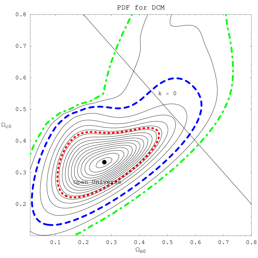
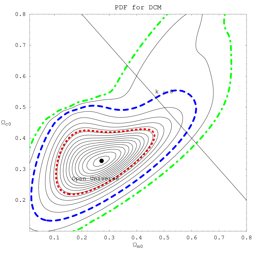
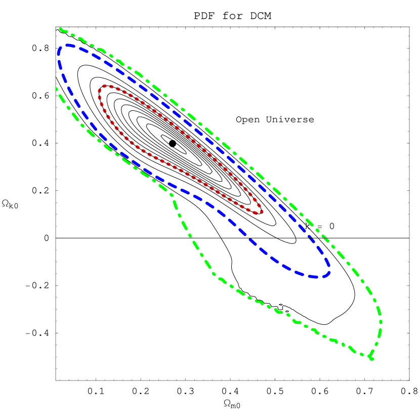
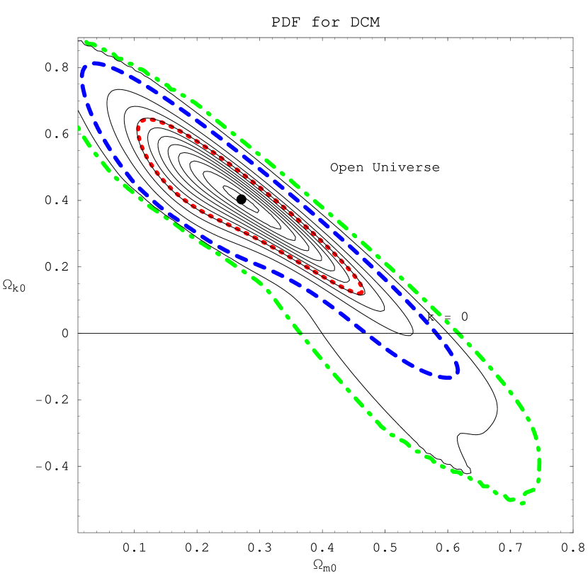
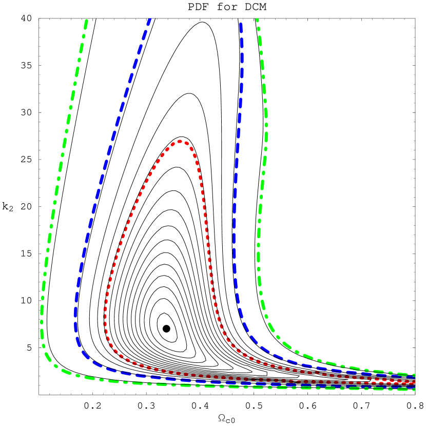
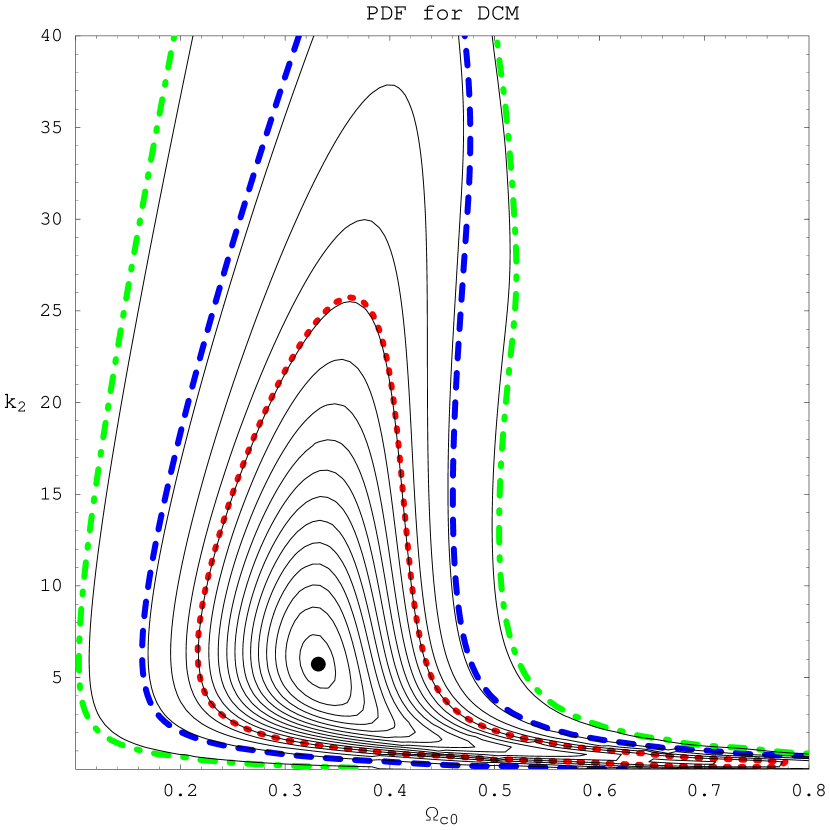
The multidimensional plot of the probability distribution is not, in general, the best way to have an overview of the results. However, we can construct a two dimensional probability distribution, integrating in two of the parameters. In figure $1$, we display the Probability Density Function, PDF, after integrating the distribution (17) in the variables $H_{0}$ and $k_{2}$: a two-dimensional probability distribution is obtained for the variables $\Omega_{m0}$ and $\Omega_{c0}$, and with $k_{1}=0$ and $1.0$. The plots show the confidence regions at $1\sigma$ ($68\%$), $2\sigma$ ($95\%$) and $3\sigma$ ($99\%$) levels. This two-dimensional probability distribution reveals that the matter density parameters have their higher probability around $\Omega_{m0},\Omega_{c0}\sim 0.3$. An open model is clearly preferred. This is also evident in figure $2$, where the two-dimensional probability distribution for $\Omega_{k0}$ and $\Omega_{m0}$ is shown. Such preference for an open model contrast strongly with a similar analysis for the $\Lambda CDM$ and Chaplygin gas models, for which a closed universe is clearly preferred [7]. As the value of $k_{1}$ grows, a low density universe becomes more favoured, as it can be seen in table $1$. In this table, we include also the case $k_{1}=0.5$ to show more explicitely that the parameter estimations change very slightly with $k_{1}$.

In figure $3$, the two-dimensional PDF is displayed when we integrate on $\Omega_{m0}$ and $H_{0}$, remaining with $k_{2}$ and $\Omega_{c0}$. As in the preceding case, a low density parameter for the dark energy component is preferred. What is specially interesting is that the values of $k_{2}$ larger than $1$ and until around $40$ have higher probabilities. This means that that a phantom scenario is clearly favoured. The peak of probability for $k_{2}$ occurs near $5-6$. As the value of $k_{1}$ increases, the peak probability for $k_{2}$ occurs at a lower value.

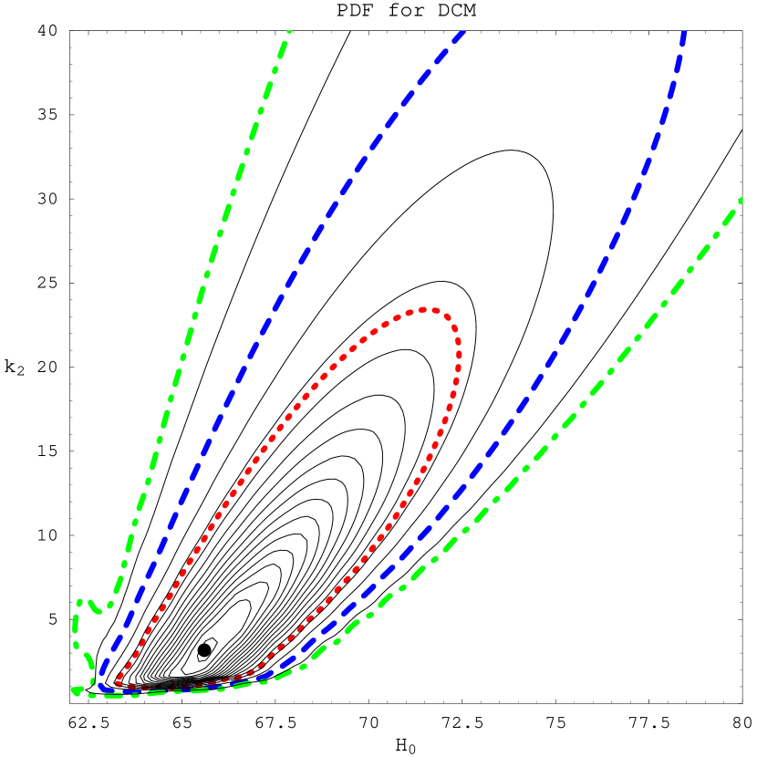
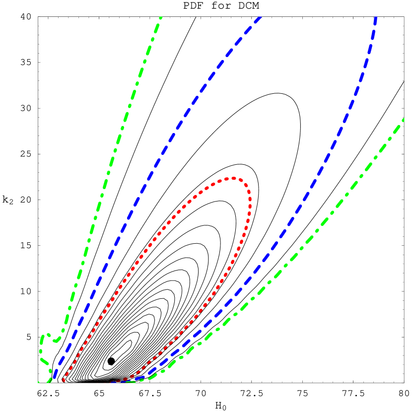
In figure $4$, the two-dimensional PDF is displayed when we integrate on $\Omega_{m0}$ and $\Omega_{c0}$, obtaining a two-dimensional graphic for $k_{2}$ and $H_{0}$. It is interesting to note, now, that regions around $H_{0}\sim 70km/Mpc.s$ are preferred. This may reconcile the estimations obtained using supernova with those obtained using CMB and matter clustering, which indicates $H_{0}$ around $72km/Mpc.s$ [6, 22]. The prefered value for $H_{0}$ depends very little on $k_{1}$.

Figure 5: The plots of the PDF as function of $\Omega_{m0}$ for the two component model, for $k_{1}=0$ and $1.0$. The joint PDF peak is shown by the large dot, the confidence regions of $1\,\sigma$ ($68,27\%$) by the dotted line, the $2\,\sigma$ ($95,45\%$) in dashed line and the $3\,\sigma$ ($99,73\%$) in dashed-dotted line.

Figure 6: The plots of the PDF as function of $(\Omega_{c0})$ for the two component model, for $k_{1}=0$ and $1.0$. The joint PDF peak is shown by the large dot, the confidence regions of $1\,\sigma$ ($68,27\%$) by the dotted line, the $2\,\sigma$ ($95,45\%$) in dashed line and the $3\,\sigma$ ($99,73\%$) in dashed-dotted line.

Figure 7: The plots of the PDF as function of $(k_{2})$ for the two component model, for $k_{1}=0$ and $1.0$. The joint PDF peak is shown by the large dot, the confidence regions of $1\,\sigma$ ($68,27\%$) by the dotted line, the $2\,\sigma$ ($95,45\%$) in dashed line and the $3\,\sigma$ ($99,73\%$) in dashed-dotted line.

Figure 8: The plots of the PDF as function of $(h)$ for the two component model, for $k_{1}=0$ and $1.0$. The joint PDF peak is shown by the large dot, the confidence regions of $1\,\sigma$ ($68,27\%$) by the dotted line, the $2\,\sigma$ ($95,45\%$) in dashed line and the $3\,\sigma$ ($99,73\%$) in dashed-dotted line.

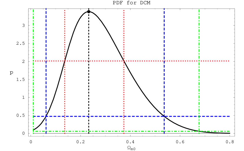
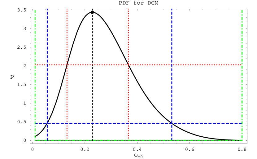
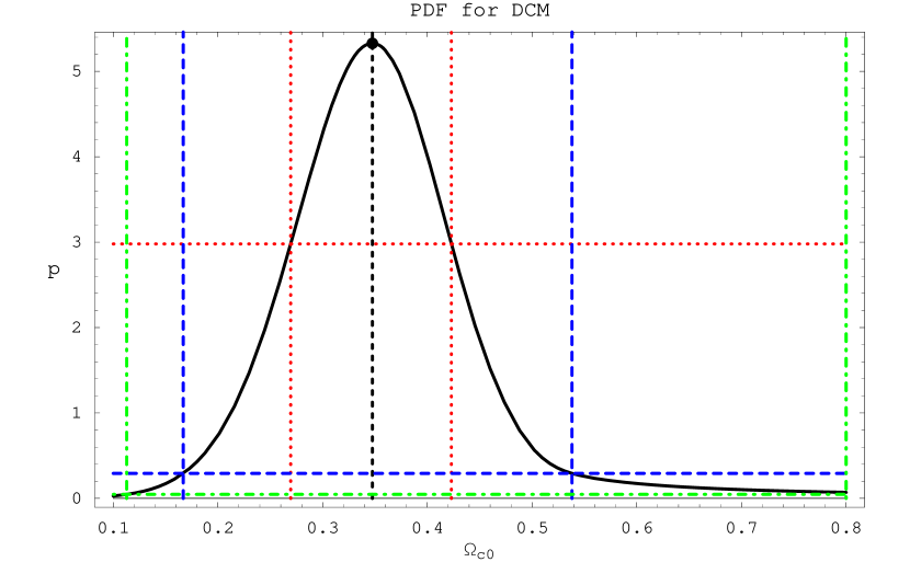
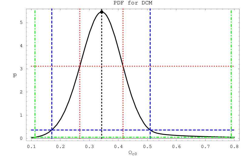
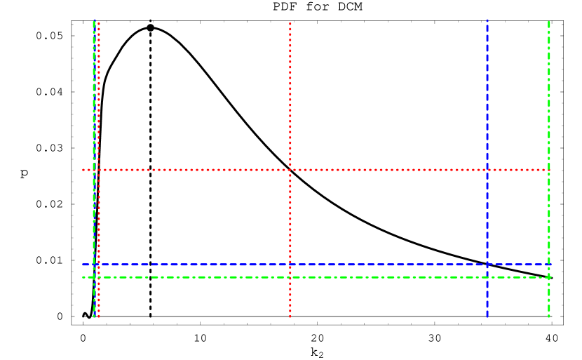
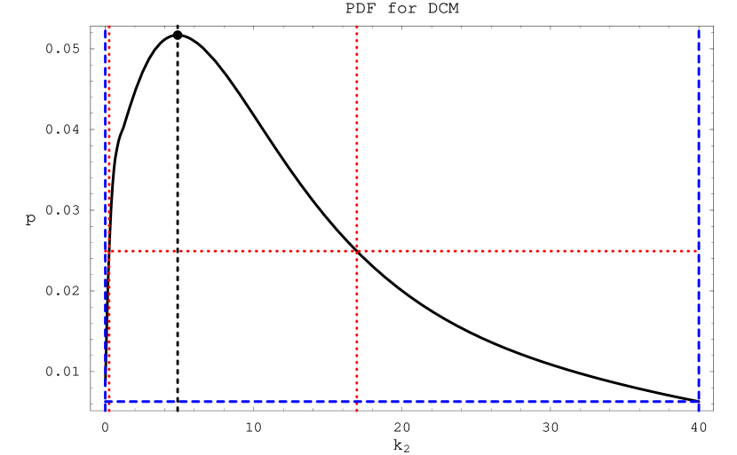
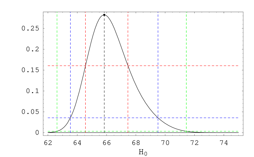
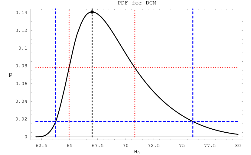
A more precise estimation of the parameters can be obtained by evaluating the one-dimensional PDF, by integrating on the three other parameters. The results are displayed in figures $5$, $6$, $7$ and $8$, and confirm what has been said based on the two-dimensional graphics. The error bars at $1\sigma$, $2\sigma$ and $3\sigma$ confidence levels are indicated. For the matter density parameter, its preferred value varies from $\Omega_{m0}=0.233$ for $k_{1}=0$ to $\Omega_{m0}=0.228$, for $k_{1}=1.0$, with a very limited dispersion. The preferred value for $\Omega_{c0}$ decreases also from $0.347$ to $0.343$. For $H_{0}$, the preferred value remains $H_{0}=67.01km/s\cdot Mpc$ with a small dispersion. However, for $k_{2}$, the preferred value varies from $k_{2}=5.75$ for $k_{1}=0$ to $k_{2}=4.88$ for $k_{1}=1.0$. However, the dispersion is extremely large. Observe that $k_{1}=0$ implies that our model reduces to a single component dark energy fluid. In this case, phantom fluids ($k_{2}>1$) are clearly preferred. Hence, an open universe, dominated by a phantom field, is a generic prediction of the model. Notice that the age of the universe is compatible with other astrophysical estimations, remaining around $13.6\,Gy$.

In order to make a proper comparison, the same analysis for the $\Lambda$CDM, using the same supernova sample, leads to $\Omega_{m0}=1.01^{+1.08}_{-0.085}$ and $H_{0}=65.0^{+1.78}_{-1.74}\,km/s\cdot Mpc$ [7]. Hence, the double component fluid model exploited here predicts a low density universe in strong contrast with the $\Lambda CDM$ model. The lowest value for the $\chi^{2}$ is $1.10$ four the double component model, and $1.11$ for the $\Lambda CDM$ model. This shows that the double component model is quite competitive.

$k_{1}$	0.0	0.5	1.0
$\Omega_{m0}$	$0.233^{+0.303}_{-0.171}$	$0.231^{+0.305}_{-0.172}$	$0.228^{+0.0.304}_{-0.172}$
$\Omega_{c0}$	$0.347^{+0.191}_{-0.181}$	$0.345^{+0.180}_{-0.178}$	$0.343^{+0.167}_{-0.172}$
$\Omega_{k0}$	$0.408^{+0.317}_{-0.467}$	$0.412^{+0.317}_{-0.457}$	$0.415^{+0.318}_{-0.439}$
$H_{0}$	$67.01^{+8.80}_{-3.21}$	$67.01^{+8.89}_{-3.24}$	$67.01^{+8.97}_{-3.24}$
$k_{2}$	$5.75^{+28.74}_{-4.75}$	$5.35^{+28.89}_{-4.85}$	$4.88^{+35.12}_{-4.88}$
$t_{0}$	$13.64^{+1.20}_{-0.74}$	$13.65^{+1.20}_{-0.75}$	$13.65^{+1.22}_{-.075}$

Table 1: Estimated values for $\Omega_{m0}$, $\Omega{c0}$, $\Omega_{k0}$, $H_{0}$, $k_{2}$ and $t_{0}$ for three different values of $k_{1}$, at $2\sigma$ level.

4 Conclusion

In this work, we have explored the possibility that the dark energy has an equation of state given by (1). This proposal has already been explored in reference [17], but restricting one of the components to behave like a cosmological constant: a two-component fluid, which is a ”variation” around a cosmological constant, has been analysed. Here, we alleviate this restriction, but introducing another one: the linear component can have any barotropic index, but the second component must vary as the square root of the density. This allows us to obtain an analytical expression for the evolution of the Universe, at least for a flat spatial section. This analytic expression reveals that it is possible to have an asymptotically de Sitter phase, for $p<0$ and $k_{2}<1$, even if only $k_{2}=1$ represents the cosmological constant. This is an intriguing aspect of the model. For $k_{2}>1$ there is always a big rip.

The restriction in the polytropic factor $\alpha$ seems not to be so relevant in view of the results of reference [17]: if the second component obeys a polytropic power law, there is a strong degeneracy on the polytropic factor, and almost any value of the power is allowed.

Our results indicate an open universe with a matter density parameter around $\Omega_{m0}\sim 0.3$, with a similar estimation for the dark energy component. The $\Lambda CDM$ model favours a closed universe. On the other hand, the predicted value for the Hubble parameter is more consistent with other observational tests, like CMB, that is, $H_{0}\sim 67\,km/s\cdot Mpc$ [23]. For the barotropic index in the two-component fluid $k_{2}$, the results indicate that $k_{2}>1$ is highly favoured. The dispersion is very high, but tends still to favour a phantom scenario. As the component index $k_{1}$ increases, the preferred value of $k_{2}$ decreases slightly.

It must be remarked that the model described here exhibits a $\chi^{2}$ slightly smaller than for the $\Lambda CDM$ model. This shows that the model is quite competitive. In our opinion, even if a phantom scenario is clearly preferred, the fact of predicting a low density universe is interesting in its own, mainly when compared with the analysis of clustering of matter in the universe.

Acknowledgments: We thank the anonymous referee who has suggested us, besides other remarks, to consider the non-flat case, what has led to new interesting results with respect to the previous version of the paper. We thank also CNPq (Brazil) and CAPES (Brazil) for partial financial support. F.C. and J.F.V.R. thank also FAPERJ (Brazil) for partial financial support. We thank Roberto Colistete Jr. and Martin Makler for their critical remarks.

References

- [1] A.G. Riess et al., Astron. J. 116, 1009(1998); S. Perlmutter et al., Astrophys. J. 517, 565(1999).
- [2] J.L. Tonry et al, Astrophys. J. 594, 1(2003).
- [3] A.G. Riess, Astrophys. J. 607, 665(2004).
- [4] P. Astier et al., Astron. Astrophys. 447, 31(2006).
- [5] L. Verde et al., Astrophys. J. Suppl. 148, 195(2003).
- [6] M. Tegmark et al., Astrophys. J. 606, 702(2004).
- [7] R. Colistete Jr, J. C. Fabris, S.V.B. Gonçalves and P.E. de Souza, Int. J. Mod. Phys. D13, 669(2004); R. Colistete Jr., J. C. Fabris and S.V.B. Gonçalves, Int. J. Mod. Phys. D14, 775(2005); R. Colistete Jr. and J. C. Fabris, Class. Quant. Grav. 22, 2813(2005).
- [8] M. Tegmark et al., Phys. Rev. D69, 103501(2004).
- [9] V. Sahni, Lect. Notes Phys. 653, 141(2004).
- [10] S. Hannestad and E. Mortsell, JCAP 0409, 001 (2004); U. Alam, V. Sahni, T.D. Saini and A.A. Starobinsky, Mon. Not. R. Astron. Soc. 354, 275 (2004); S.W. Allen et al., Mon. Not. R. Astron. Soc. 353, 457 (2004).
- [11] H.K. Jassal, J.S. Bagla and T. Padmanabhan, The vanishing of phantom menace, astro-ph/0601389.
- [12] A.Yu. Kamenschik, U. Moschella and V. Pasquier, Phys. Lett. B511, 265 (2001); J.C. Fabris, S.V.B. Gonçalves and P.E. de Souza, Gen. Rel. Grav. 34, 53 (2002); N. Bilic, G.B. Tupper and R.D. Viollier, Phys. Lett. 535, 17 (2002); M.C. Bento, O. Bertolami and A.A. Sen, Phys. Rev. D66, 043507 (2002).
- [13] S. Mukherjee, B.C. Paul, N.K. Dadhich, S.D. Maharaj and A. Beesham, Emergent universes with exotic matter, gr-qc/0605134.
- [14] H.B. Benaoum, Accelerated universe from modified Chaplygin gas and tachyonic fluid, hep-th/0205140.
- [15] U. Debnath, A. Banerjee and S. Chakraborty, Class. Quant. Grav. 21, 5609 (2004).
- [16] W. Chakraborty and U. Debnath, Is the modified Chaplygin gas along with barotropic fluid responsible for acceleration of the universe?, gr-qc/0611094.
- [17] J.S. Alcaniz and H. Stefancic, ”Expansion” around the vacuum: how far can we go from ?, astro-ph/0512622.
- [18] J.C. Fabris and J. Martin, Phys. Rev. D55, 5205 (1997).
- [19] S. Weinberg, Gravitation and cosmology, Wiley, New York( 1972).
- [20] P. Coles and F. Lucchin, Cosmology, Wiley, New York (1995).
- [21] R. Colistete Jr., BayEsian Tools for Observational Cosmology using SNe Ia (BETOCS), available on the Internet site http://www.RobertoColistete.net/BETOCS, (2006).
- [22] D.N. Spergel et al., Wilkinson microwave anisotropy probe (WMAP) three years results: implications to cosmology, astro-ph/0603449.
- [23] D.N. Spergel et al., Astrophys. J. Suppl. 148, 175(2003).