Cosmic Calibration

Abstract

The complexity and accuracy of current and future “precision cosmology” observational campaigns has made it essential to develop an efficient technique for directly combining simulation and observational datasets to determine cosmological and model parameters; a procedure we term calibration. Once a satisfactory calibration of the underlying cosmological model is achieved, independent predictions for new observations become possible. For this procedure to be effective, robust characterization of the uncertainty in the calibration process is highly desirable. In this Letter, we describe a statistical methodology which can achieve both of these goals. An application example based around dark matter structure formation simulations and a synthetic mass power spectrum dataset is used to demonstrate the approach.

                                                                                                                                     LA-UR-06-2320

1 Introduction

It is widely recognized that, beginning in the last decade, a transition to an era of “precision cosmology” is well underway. Ongoing and upcoming surveys such as the Wilkinson Microwave Anisotropy Probe (WMAP, Spergel et al. 2006), the Sloan Digital Sky Survey (SDSS, Adelman-McCarthy et al. 2006), Planck, the Dark Energy Survey (DES), the Joint Dark Energy Mission (JDEM), the Large Synoptic Survey Telescope (LSST), and Pan-STARRS constitute superb sources of cosmological statistics. These sources include (galaxy, cluster, and mass) power spectra and cluster mass functions, from which roughly 25 cosmological parameters have to be constrained (see, e.g., Spergel et al. 2006, Tegmark et al. 2003, Abazajian et al. 2005). The promised accuracy from future observations is remarkable, as some parameters can be measured at the 1% level or better, posing a major challenge to cosmological theory. Predictions and analysis methods must at least match – and preferably substantially exceed – the observational accuracy. For many observables, this can only be achieved by simulations incorporating physical effects beyond the reach of analytic modeling.

Cosmological simulations already play a key role in the design and interpretation of observations. Controlling systematics is a necessary first step, followed by combining simulations with observations to extract cosmological and model parameters. This cannot be accomplished by brute force. For example, if every parameter is sampled only ten times in a twenty-dimensional parameter space, it would require $10^{20}$ large-scale simulations, which is currently – and in the near-term – quite impossible. Even the variation of only a subset of the parameters over a sufficient range is infeasible. The need to develop and employ reliable statistical methods to determine and constrain parameters robustly is therefore manifest.

In this Letter we describe a statistical framework to determine cosmological and model parameters and associated uncertainties from simulations and observational data (for an overview of the basic ideas see, e.g., Kennedy & O’Hagan 2001 and Goldstein & Rougier 2004). The framework integrates a set of interlocking procedures: (i) simulation design – the determination of the parameter settings at which to carry out the simulations; (ii) emulation – given simulation output at the input parameter settings, how to estimate the output at new, untried settings; (iii) uncertainty and sensitivity analysis – determining the variations in simulation output due to uncertainty or changes in the input parameters; (iv) calibration – combining observations (with known errors) and simulations to estimate parameter values consistent with the observations, including the associated uncertainty; (v) prediction – using the calibrated simulator to predict new cosmological results with a set of uncertainty bounds.

For concreteness, we discuss the framework methodology in terms of a simple example application: Estimation of five parameters from dark matter structure formation simulations and a synthetic set of “WMAP + SDSS” measurements of the matter power spectrum. A detailed description will be provided elsewhere (S. Habib et al. in preparation).

2 The Statistical Framework

We employ a Bayesian framework to update prior probability distributions on cosmological parameters given observational data. Denoting these parameters collectively by $\theta$ and the observed power spectrum data by a vector $y_{\rm obs}$, we model the data as:

$$y_{\rm obs}=\eta(\theta)+\epsilon,$$ (1)

where $\eta(\theta)$ denotes the simulation output at input setting $\theta$, and $\epsilon\sim N(0,\Sigma_{y})$ where $\Sigma_{y}$ describes the error structure of the observations and any potential systematic differences between the simulated and observed data.

Standard Bayesian estimation (Jeffreys 1961) proceeds using the likelihood

$$L(y_{\rm obs}|\theta)\propto|\Sigma_{y}|^{-1/2}{\exp}\{-\frac{1}{2}[y_{\rm obs}-\eta(\theta)]^{T}\Sigma_{y}^{-1}[y_{\rm obs}-\eta(\theta)]\},$$ (2)

and a prior $\pi(\theta)$ to form the posterior distribution on $\theta$:

$$\pi(\theta|y_{\rm obs})\propto L(y_{\rm obs}|\theta)\pi(\theta).$$ (3)

Because the resulting posterior distributions are not in any easily recognized closed form, they must be explored numerically, usually using Markov Chain Monte Carlo (MCMC) techniques (Besag et al. 1995). This procedure requires running the (potentially very expensive) simulation codes many thousands of times as the $\theta$-space is explored. However, only a limited number ($\sim 100?\,\sim 1000$?) of runs may be feasible. Therefore, efficiently combining Bayesian methods with simulations requires a representation of the code output (emulator) that can be sampled many thousands of times during the course of the MCMC in lieu of running the actual code. When queried at an input setting where a code run is available, the emulator should reproduce the output of the code. At other input settings, the emulator effectively interpolates nearby code runs while including uncertainty due to the lack of complete knowledge of the code output. The selection of input settings in the simulation design must be sufficiently dense that the emulator can accurately mimic the code output, and also be sufficiently sparse that the simulation campaign is computationally tractable.

Systematic design of simulation procedures is reviewed in Santner et al. (2003). We use orthogonal array-based Latin hypercube sampling Tang (1993) to fix 128 input settings over the five parameters. This approach takes an orthogonal array design – which ensures that all lower-dimensional projections have desirable space-filling properties – and modifies it so that it is also a Latin hypercube, the most efficient stratified sampling strategy.

The code output for the $i$th input setting is a power spectrum, $y^{(i)}(k)=\eta(\theta_{i})$, viewed as a column vector over the $n_{k}$ points in $k$ space. Each of the resulting $n_{s}=128$ output spectra is loaded into a single $n_{k}\times n_{s}$ matrix: $y_{\rm sims}=[y^{(1)}|y^{(2)}|\ldots|y^{(n_{s})}].$ This matrix is then subjected to a singular value decomposition (SVD) to find an efficient empirical orthogonal representation of the simulation outputs: $[y_{\rm sims}]_{ij}=[USV^{T}]_{ij}=\sum_{p=1}^{n_{s}}\lambda_{p}[\alpha_{p}]_{i}w_{p}(\theta_{j})$ where the $\alpha_{p}$’s are $n_{k}\times 1$ orthogonal basis vectors in the simulation output space (columns of $U$), the $\lambda_{i}$’s are the singular values of the simulation matrix, and each principal component (PC) weight $w_{p}(\theta)$ is a $1\times n_{s}$ row vector in the parameter space (columns of $V$). Usually the first few singular values dominate the remainder, allowing us to keep only a few of the principal components in the analysis. In what follows, we have kept five PC’s.

The SVD gives the PC weights at the design input settings $(\theta_{1},\theta_{2},\cdots,\theta_{n_{s}})$. However, in the course of the MCMC, we need the PC weights at intermediate input settings. We construct the emulator by putting a spatial Gaussian Process (GP) model on each PC weight (Sacks et al. 1989, MacKay 1998), a nonlinear interpolation scheme that works directly on the space of functions. This allows the emulator to smoothly interpolate the predicted code output between the design settings, giving an efficient probabilistic representation of the prediction uncertainty. The spatial parameters controlling the GP on each component weight are estimated in the course of the MCMC, thereby constructing the emulator as needed during the calibration analysis. Details of the procedures used in our code are being reported elsewhere in the literature. For recent examples of these techniques used in practice, see Higdon et al. (2004).

3 Parameter Estimation and the Nonlinear Matter Power Spectrum

In order to give an explicit demonstration of the approach, we first generate a synthetic observational dataset from simulations. The key advantage of doing this is that the underlying set of cosmological parameters are known, allowing a direct test of the statistical procedure. To generate the “observations” we begin with a smooth power spectrum computed by running ten realizations of the same cosmology with the parallel particle mesh (PM) code MC² (Cf. Heitmann et al. 2005 for code information and comparison results) and averaging over the results. The initial conditions are set using CMBFAST Seljak & Zaldarriaga (1996). We restrict our study to the linear and quasi-linear regime relevant to large-scale structure surveys; the force resolution of the PM-code accurately resolves the scales of interest.

Figure 1: Subset of the 128 simulated power spectra and the synthetic dataset. The black line is the spectrum from which the synthetic data were derived.

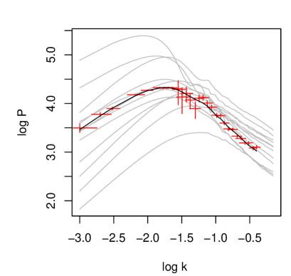
We form a single power spectrum by attaching the linear $P_{L}(k),\;0.001h$Mpc${}^{-1}\leq k\leq 0.1h$Mpc^-1 (growth specified by linear theory), to the power spectrum from simulations $P_{N}(k)$ at $k=0.1h$Mpc^-1. Next, 28 points from this combined power spectrum are picked, spaced roughly in the same bins as in a real dataset. The error bars are set by values typical for cosmic microwave background (CMB) experiments such as WMAP (Spergel et al. 2006) in the low-$k$ range, transitioning to values typical of surveys such as SDSS (Adelman-McCarthy et al. 2006) at higher $k$. Finally, points are moved off the base power spectrum according to a Gaussian distribution with a 1-sigma confidence, as shown in Figure 1. Note that for this test demonstration we are assuming that galaxy bias has already been incorporated in the measurement. In a more realistic situation, the bias would be included as part of the modeling process. Note also that the choice of a homogeneous observational dataset here is merely for convenience. For a heterogeneous dataset such as CMB $C_{l}$’s combined with $P(k)$ measured from the galaxy distribution, $y_{obs}$ [Cf. Eqn. (1)] would also contain the CMB results and the simulations underlying $\eta(\theta)$ would include runs of (say) CMBFAST.

We consider the following five cosmological parameters: $\theta=(n,h,\sigma_{8},\Omega_{\rm CDM},\Omega_{\rm b})$. We assume a flat $\Lambda$CDM universe with $\theta=(0.99,0.71,0.84,0.27,0.044)$ to make the synthetic observations (black line in Figure 1). To determine the simulation design we must fix the range that the input parameters should be varied over. To this end, we assume independent, flat priors over the ranges: $0.8\leq n\leq 1.4$, $0.5\leq h\leq 1.1$, $0.6\leq\sigma_{8}\leq 1.6$, $0.05\leq\Omega_{\rm CDM}\leq 0.6$, and $0.02\leq\Omega_{\rm b}\leq 0.12$. The simulation design prescribes a set of 128 input settings. This number of simulations, as we show below, yields an emulator with performance at the few percent level, sufficient for our present purposes.

Each run is carried out with 128³ particles on a 512³ grid for a 450$h^{-1}$Mpc box, guaranteeing sufficient force resolution for the scales of interest. To limit systematic biases, different seeds are used to generate the initial Gaussian random field for each simulation. Cosmic variance is minimized by matching the numerical to the linear power spectrum in the linear regime near the $\Lambda$CDM power spectrum peak. We show a subset of the 128 power spectra in Figure 1. The emulator is now built as described above – note that the emulator is called only as needed by the MCMC analysis in the calibration process.

4 Results

Figure 2: Posterior density for the parameter vector $\theta$. The diagonal gives estimates of the univariate marginal pdfs for each component; blue: results from the entire synthetic dataset; green using only the linear regime ($k<0.1h{\rm Mpc}^{-1}$). Off-diagonal images show estimates of the bivariate marginal pdfs: upper triangle for the entire dataset, lower triangle for the linear regime. The lines give estimates of the 90% highest posterior density region. Again, blue is from using the entire dataset; green from using only the linear regime. The dots show the actual parameter values used to generate the synthetic observations.

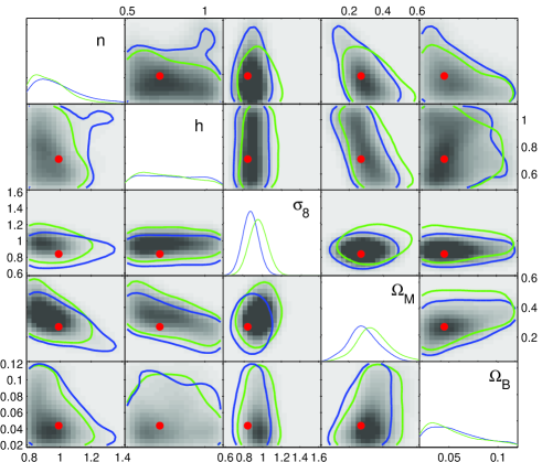
The posterior distribution of the five cosmological parameters is depicted in Figure 2. The diagonal displays the univariate, marginal pdfs for each of the parameters, while the off-diagonal plots show estimated 2-d marginal densities, along with 90% probability contours. For comparison, Table 1 gives the mean value of the parameters along with the estimated uncertainty, as well as the “true” value for each parameter. These posterior estimates are obtained under two separate formulations – one which uses all of the synthetic observation data, and one which uses only the observations in the linear regime for which $k<0.1h$Mpc^-1. The green pdfs and contours in Figure 2 show the posterior results including information only from the linear regime, whereas the blue pdfs and the contours result from an analysis of the full nonlinear power spectrum. Because of the limited observational dynamic range, using only the linear regime results in systematic shifts from the “true” answers, albeit within the quoted uncertainties. Overall, we find $\Omega_{\rm CDM}$ and $\sigma_{8}$ to be very well determined. The full nonlinear analysis over the entire $k$-range significantly improves the accuracy for $\sigma_{8}$ and $\Omega_{\rm CDM}$ as well as the precision of the constraint for $\sigma_{8}$ (see Table 1). While the synthetic dataset provides information about the remaining three parameters, $n$, $h$, and $\Omega_{\rm b}$, they are not as well constrained as is to be expected from an analysis restricted to the matter power spectrum only. Note that the linear analysis underestimates the uncertainty in $n$.

Figure 3: Evaluation of the emulator fit. Left: Three simulations (black dots) and the corresponding response surface fits (green lines) obtained after holding out the simulation to be predicted and training the response surface on the remaining 127 simulations. Right: Residual (simulation $\log P-$ response surface) from holdout predictions (i.e. the simulation being predicted is not used to estimate the response surface). The central gray region contains the middle 50% of the residuals; the wider light gray region, the middle 90%.

Table 1: Parameter Constraints

Param.	Meannonlin	Meanlin	True Value
n	$0.991^{+0.276}_{-0.171}$	$0.940^{+0.218}_{-0.132}$	0.99
h	$0.786^{+0.2823}_{-0.259}$	$0.765^{+0.287}_{-0.232}$	0.71
$\sigma_{8}$	$0.882^{+0.082}_{-0.077}$	$0.962^{+0.121}_{-0.108}$	0.84
$\Omega_{\rm CDM}$	$0.287^{+0.138}_{-0.133}$	$0.343^{+0.156}_{-0.130}$	0.27
$\Omega_{\rm b}$	$0.057^{+0.052}_{-0.034}$	$0.054^{+0.052}_{-0.031}$	0.044

Figure 4: Sensitivity of the computed power spectrum $\log P$ to changes in input parameters. Here, the response surface is used to compute the change in $\log P$ as each parameter, in turn, is varied from its lower bound to its upper bound while the other parameters are held at their midpoints.

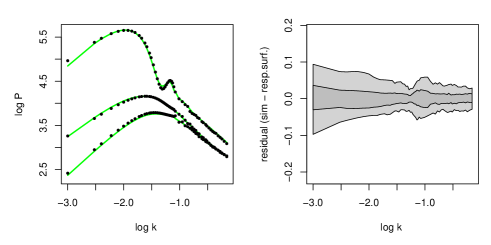
The posterior distribution describes the uncertainty regarding the parameter vector $\theta$ as well as statistical variance and correlation parameters that control the response surface model. Once these posterior samples have been produced, it is straightforward to generate posterior realizations of the emulator to assess its adequacy in modeling the simulated output. The accuracy of the emulator was estimated by excluding individual simulation runs and building a new emulator based on the remaining 127 power spectra. The emulator predictions can now be compared against the actual simulation output of the excluded run. Three examples of applying this procedure are shown in the left plot in Figure 3. The accuracy of the emulator turns out to be extremely good, at the level of a few percent, which is very adequate for the present analysis. The right panel in Figure 3 summarizes the residuals for all 128 simulations – the central gray band delineates the middle 50% of the residuals; the light gray band delineates the middle 90%. Gaussian process models offer a number of advantages over other methods for modeling simulation output: they do not require runs over a grid of input settings; they allow for interpolation of the simulation output; they can accommodate fairly general interactions between input parameters; and typically outperform other modeling approaches. For example, the GP model gives substantially better predictions as compared to a quadratic response surface model, a generalized additive model (GAM), or a multivariate additive regression spline model (MARS) (Hastie et al. 2001).

The fitted emulator can be used to explore the sensitivity of the simulation output to changes in the cosmological parameters. Figure 4 shows how the log of the power spectrum changes as one parameter is varied, the others being fixed at their prior midpoints. Both $\sigma_{8}$ and $\Omega_{\rm CDM}$ have a large impact when varied over their prior ranges. Hence it is not surprising that the posterior distribution for these two parameters are the most constrained by the observed data. Figure 4 also suggests that while most parameters affect the power spectrum in the linear regime ($k<0.1h{\rm Mpc}^{-1}$), only $\sigma_{8}$ affects the power spectrum in the nonlinear regime ($k>0.1h{\rm Mpc}^{-1}$). Thus, while additional data in the nonlinear regime is likely to help constrain $\sigma_{8}$, it will not greatly reduce uncertainty in the other four parameters.

5 Conclusion and Outlook

We have introduced a new, very powerful method for determining cosmological and model parameters from simulations and observations. The key idea is to extract maximum utility from a necessarily finite set of expensive simulations. The implementation of this idea includes several valuable features: (i) a design to optimally sample the simulation parameter space; (ii) an accurate emulator capable of generating the required outputs in between the sampled simulation points; (iii) an uncertainty and sensitivity analysis; (iv) the parameter constraints themselves, with associated uncertainty bounds.

In order to demonstrate the basic approach, we used a set of 128 dark matter structure formation simulations and a homogeneous synthetic “observational” dataset to determine five cosmological parameters. The next step is to use the framework for analyses of real data, especially of combined datasets such as the CMB and large scale structure observations.

There are many ways to enhance the method and improve its performance. One is the melding of information from codes with different degrees of resolution and input physics, such as in the extraction of information about the mass distribution from the Lyman-$\alpha$ forest. Here, complex hydrodynamics simulations are certainly desirable, but much faster approximate methods such as hydro-particle mesh (HPM) are available. Thus, a first analysis based on HPM can be performed, narrowing the parameter range of interest sufficiently to make hydro runs feasible. Interesting offshoots of the methodology include the exploitation of certain intermediate results. For instance, a large set of N-body simulations can be performed with several input parameters such as the equation of state for dark energy. An emulator can then be constructed from these and publicly released. This emulator can then be conveniently used instead of real simulations for planning observations and data analysis.

References

- Abazajian et al. (2005) Abazajian, K. et al. 2005, ApJ 625, 613
- Adelman-McCarthy et al. (2006) Adelman-McCarthy, J.K. et al. 2006, ApJS, 162, 38
- Besag et al. (1995) Besag, J., Green, P., Higdon, D.A., & Mengersen, K. 1995, Stat. Sci. 10, 3
- Goldstein & Rougier (2004) Goldstein, M. and Rougier, J. 2004, SIAM J. Sci. Comput. 26, 467
- Heitmann et al. (2005) Heitmann, K., Ricker, P.M., Warren, M.S., & Habib, S. 2005, ApJS, 160, 28
- Hastie et al. (2001) Hastie, T., Tibshirani, R., & Friedman, J. 2001, The Elements of Statistical Learning: Data Mining, Inference, and Prediction (Springer)
- Higdon et al. (2004) Higdon, D.A. et al. 2004, SIAM J. Sci. Comput. 26, 448
- Jeffreys (1961) Jeffreys, H. 1961, Theory of Probability (Oxford)
- Kennedy & O’Hagan (2001) Kennedy, M.C. & O’Hagan, A. 2001, J. Royal Stat. Soc. B, 63, Part 3, 425
- MacKay (1998) MacKay, D.J.C. 1998 in Neural Networks and Machine Learning, ed. Bishop, C.M., NATO ASI Series (Kluwer)
- Sacks et al. (1989) Sacks, J., Welch, W.J., Mitchell, T.J., & Wynn, H.P. 1989, Stat. Sci, 4, 409
- Santer et al. (2003) Santer, T.J., Williams, B.J., & Notz, W. 2003, The Design and Analysis of Computer Experiments (New York: Springer)
- Seljak & Zaldarriaga (1996) Seljak, U. & Zaldarriga, M. 1996 ApJ, 469, 437
- Spergel et al. (2006) Spergel, D.N. et al. astro-ph/0603449, ApJ, submitted
- Tang (1993) Tang, B., 1993 J. Am. Stat. Assn., 88, 1392
- Tegmark et al. (2004) Tegmark, M. et al. 2004, Phys. Rev. D, 69, 103501