Search for Diffuse Astrophysical Neutrino Flux Using Ultra–High-Energy Upward-going Muons in Super-Kamiokande I

Abstract

Many astrophysical models predict a diffuse flux of high-energy neutrinos from active galactic nuclei and other extra-galactic sources. At muon energies above 1 TeV, the upward-going muon flux induced by neutrinos from active galactic nuclei is expected to exceed the flux due to atmospheric neutrinos. We have performed a search for this astrophysical neutrino flux by looking for upward-going muons in the highest energy data sample from the Super-Kamiokande detector using 1679.6 live days of data. We found one extremely high energy upward-going muon event, compared with an expected atmospheric neutrino background of $0.46\pm 0.23$ events. Using this result, we set an upper limit on the diffuse flux of upward-going muons due to neutrinos from astrophysical sources in the muon energy range 3.16–100 TeV.

1. Introduction

The GeV-PeV energy range is unexplored territory for neutrino astronomy — observations of neutrinos at these energies will open a new window on the high energy universe. A wide variety of astrophysical phenomena are expected to produce extremely high energy neutrinos, ranging from active galactic nuclei (AGNs) and gamma-ray bursts (GRBs; Halzen & Hooper 2002; Gaisser et al. 1995) to more exotic sources such as dark matter annihilation or decays of topological defects (Staśto 2004).

The flux of neutrinos at such high energies is quite small; therefore, large-scale detectors are required. One effective technique for observing high-energy neutrinos with an underground detector is to look for muons produced by $\nu_{\mu}$ or $\bar{\nu}_{\mu}$ interacting in the surrounding rock. (Throughout this paper, “muons” will refer to both $\mu^{+}$ and ${\mu^{-}}$.) The muon range in rock increases with muon energy, which expands the effective interaction volume for high-energy events. Downward-going neutrino-induced muons cannot be distinguished from the much larger flux of downward cosmic-ray muons, but since cosmic ray muons cannot travel through the entire Earth, upward-going muons are almost always neutrino-induced. Thus, upward-going muons provide a suitable high-energy neutrino signal.

At muon energies above $1-10{\rm{\;TeV}}$, the upward-going muon flux due to neutrinos from AGNs is expected to exceed the flux due to atmospheric neutrinos (Stecker & Salamon 1996; Mannheim et al. 2001). This cosmic neutrino flux could be detected either by searching for point sources of high-energy neutrinos or by detecting a diffuse, isotropic flux of neutrinos from unresolved astrophysical sources. A diffuse cosmic neutrino flux would be observed as an excess to the expected atmospheric neutrino flux at high energies. In this analysis, we focus on searching for a diffuse flux of upward-going muons due to neutrinos from astrophysical sources using the highest energy data sample in Super-Kamiokande (Super-K). This study complements other Super-K searches for astrophysical point sources of high energy neutrinos that use data over a larger energy range (Abe et al. 2006). In this paper we describe a search for evidence of a high energy astrophysical neutrino flux in Super-K’s highest energy upward-going muon sample. In § 2 we describe the Super-Kamiokande detector, and in § 3 we give the details of how we selected candidate events from Super-K’s ultra–high-energy sample. We evaluate our selection process with Monte Carlo in § 4 and calculate the observed upward-going muon flux in § 5. Sections 6 and 7 discuss the background due to the atmospheric neutrino flux. Based on the results, we set an upper limit in § 8 and conclude in § 9. Any necessary estimates and approximations have been made so that they lead to a conservative result for this upper limit.

2. The Super-Kamiokande Detector

The Super-K detector is a cylindrical 50 kiloton water Cerenkov detector, located in the Kamioka-Mozumi mine in Japan. It is 41.4 m tall and 39.3 m in diameter. The detector was constructed under the peak of Mount Ikenoyama, which provides an average rock overburden of 1000 m (2700 m water equivalent). Its geodetic location is at 36.4^∘ north, 137.3^∘ east, and altitude 370 m.

Super-K consists of two concentric, optically separated detectors. Until 2001 July the inner detector (ID) was instrumented with 11,146 inward-facing 50 cm diameter photomultiplier tubes (PMTs). The outer detector (OD) is a cylindrical shell of water surrounding the ID and is instrumented with 1885 outward-facing 20 cm diameter PMTs. Between the ID and the OD, there is a 50 cm thick shell. Photons coming from this region will not be detected by either the OD or the ID, so we refer to it as the insensitive region.

More details about the detector can be found in Fukuda et al. (2003). The data sample used in this analysis was taken from 1996 April to 2001 July, corresponding to 1679.6 days of detector livetime. This data run is referred to as SK-I.

Super-K is primarily designed to detect lower energy neutrinos from the Sun, the atmosphere, and particle accelerators but can potentially detect the extremely high energy neutrinos expected from astrophysical sources as well. This paper focuses on the events at the highest energy end of Super-K’s detection range.

3. Event Selection

The ultra–high-energy sample in SK-I consists of events that deposit $\geq 1.75\times 10^{6}$ photoelectrons (pe) in the ID. In the low-energy regime, on average about 9 pe are recorded by the ID PMTs for each MeV of energy deposited in the tank; the electronics for the ID PMTs saturate at about 300 pe. Thus an event with $\geq 1.75\times 10^{6}$ pe in the ID corresponds to a minimum energy deposition of approximately 200 GeV, but the actual energy deposition could be much higher, since the saturation effect prevents all of the produced pe from being recorded.

At high energies, muons have some probability to lose energy through radiative processes such as bremsstrahlung, resulting in an electromagnetic shower that deposits large quantities of pe in the detector. For comparison, a muon that traverses the maximum path length through the ID (50 m) but does not produce any electromagnetic showers will deposit approximately 11 GeV via ionization energy loss, corresponding to $\sim 10^{5}$ pe deposited in the ID. Thus a high-pe cutoff offers a means of selecting high energy events.

At the high-pe threshold of $\geq 1.75\times 10^{6}$ pe, the high level of saturation in the ID PMT electronics can cause Super-K’s precision muon fitting algorithms to fail. Therefore, these extremely energetic events are not included in other studies of upward-going muons in SK-I (Desai et al. 2004; Fukuda et al. 1999; Ashie et al. 2005). In this study we analyzed this ultra–high-energy data sample separately using a different fitting method based on information from the OD.

3.1. Outer Detector Linear Fit

SK-I’s ultra–high-energy data sample contains a total of 52214 events. Most of these are either very energetic downward-going cosmic-ray muons or multiple muon events where two or more downward-going muons hit the detector simultaneously. In order to select candidate upward-going muons from this sample, we applied a simple linear fit to the OD data for each event. A linear fit was done on the $z$-position of each OD PMT versus the time it fired, weighted by the total charge in the PMT. Example fits of simulated downward-going and upward-going muon events are shown in Figure 1.

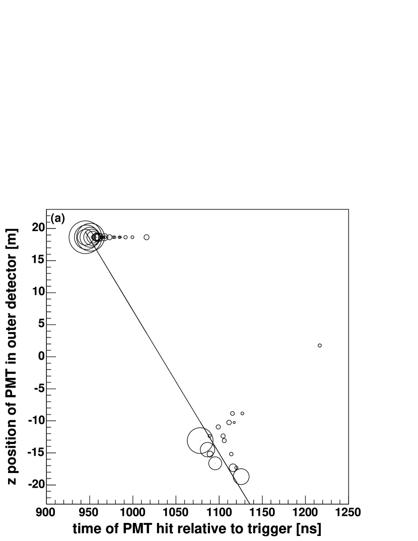
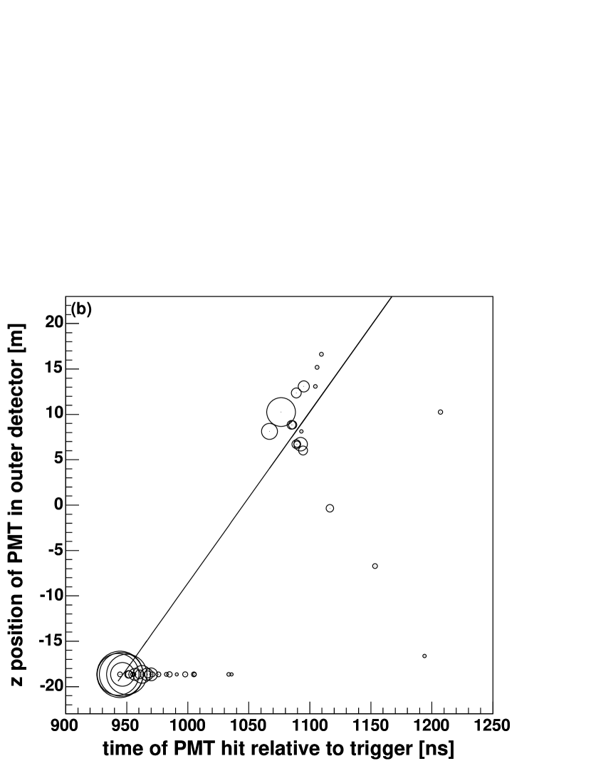
Figure 1.— (a) OD-based muon trajectory fit applied to an example MC downward-going muon event. (b) OD-based fit applied to an example MC upward-going muon event. The size of the circle around each point is proportional to the charge detected in the PMT.

The slope of this fitted line is an estimate of $-\cos{\Theta}$, where $\Theta$ is the zenith angle of the incoming muon. A positive fitted slope indicates that the muon is upward-going. A similar linear fit was done on the $x$- and $y$-positions to determine the full muon trajectory through the detector.

Since this fitting method is based on the OD (which has a lower resolution than the ID), it is not as precise as the muon fitting algorithms used in the lower energy upward-going muon analysis. However, it works even when the ID PMT electronics are completely saturated and the precision ID-based algorithms fail.

3.2. Selection Cuts

To select candidate upward-going muons, we applied the OD-based fit to all 52214 events in the ultra–high-energy data sample. A cut of $\cos{\Theta}\leq 0.1$ was used to eliminate the bulk of the downward-going single and multiple muon events. In addition, the fitted trajectory was required to have a path length of $>7{\rm{\;m}}$ in the ID.

To ensure high-quality fit results, we looked at the number of OD PMTs hit near the projected entry and exit points. For a true throughgoing muon, there will be a cluster of hit PMTs around the entry and exit points. If the fit is accurate, the projected path should pass through both of these clusters, so we made an additional cut on the number of OD PMTs hit within $10{\rm{\;m}}$ of the projected OD entry and exit points, $N_{{\rm ODentry}}$ and $N_{{\rm ODexit}}$. We required both $N_{{\rm ODentry}}$ and $N_{{\rm ODexit}}$ to be 10 or greater.

Events that do not have $N_{{\rm ODentry}}$ and $N_{{\rm ODexit}}\geq 10$ are generally either stopping muons, partially contained events, or poorly fitted throughgoing muons. Stopping muons are muons that stop in the detector and only form an OD entry cluster. They typically have energies of 1-10 GeV, well below the range of the expected astrophysical signal, so it is appropriate to discard events that look like stopping muons. Partially-contained events are neutrino interactions that take place inside the detector and only form an OD exit cluster — they are not part of the upward-going muon flux incident on the detector, so we want to discard these as well. This cut also occasionally eliminates inaccurately fitted throughgoing muon events, which reduces the efficiency somewhat but improves the accuracy of the fit results.

Another possible type of event that can masquerade as a throughgoing muon is a partially-contained event with multiple exiting particles. Such an event will create two (or more) clusters of hit PMTs in the OD, which could be mistaken as the entry and exit points of a throughgoing muon. In order to eliminate such events, we looked at the timing between the OD and ID entry points. If the event is truly a throughgoing muon, the OD PMTs near the entry point should fire before the ID PMTs. We determined OD and ID entry clusters via a simple time-based clustering method and evaluated the mean time of hits within $6{\rm{\;m}}$ of the OD and ID entry points, $t_{{\rm IDentry}}$ and $t_{{\rm ODentry}}$.

In an ideal measurement, $t_{{\rm IDentry}}<t_{{\rm ODentry}}$ would indicate that the perceived entry cluster is actually caused by an exiting particle. However, the timing determination is complicated by an effect known as prepulsing. Prepulsing occurs when there are so many photons incident on the PMT that they are not all converted to photoelectrons at the photocathode - some photons hit the first dynode instead and are converted to photoelectrons there. When this happens in an ID PMT, the PMT pulse appears earlier relative to the OD light. If this occurs for an ultra-high energy throughgoing muon event, it could cause $t_{{\rm IDentry}}-t_{{\rm ODentry}}$ to be negative. To allow for this effect, we used a fairly loose cut of $-40{\rm{\;ns}}$: if $t_{{\rm IDentry}}-t_{{\rm ODentry}}<-40{\rm{\;ns}}$, indicating very early ID light, then the event was rejected as a likely neutrino interaction in the ID.

After these cuts on $\cos{\Theta}$, path length, $N_{{\rm ODentry}}$, $N_{{\rm ODexit}}$, and $t_{{\rm IDentry}}-t_{{\rm ODentry}}$ were applied to the 52214 events in the sample, 343 candidate events remained. These remaining events were then evaluated by a visual scan and a manual direction fit by two independent researchers to select events with $\cos{\Theta}<0$.

The visual scan eliminates events that can pass the automatic reduction but are obvious to the trained human eye as noise, i.e., mainly downward-going multiple muon events and “flashers.” Multiple muon background events occur when two or more downward-going muons from an atmospheric shower pass through the detector simultaneously. They have extra energy deposition (and thus are expected to be more common in the ultra–high-energy sample) and typically give poor OD fit results due to multiple OD clusters, but they are easy to identify visually. Flashers are events caused by malfunctioning PMTs that emit light and create characteristic patterns. After the multiple muon events and flashers are removed, the manual direction fit separates truly upward-going muons from mis-fitted downward-going muons.

From the 343 candidates, only one event passed the visual scan and manual direction fit selection as being truly upward-going. The breakdown of the visual scan and manual fit classifications is shown in Table 1.

Table 1Visual scan of candidate upward-going muon events

Visual scan classification	Number of events
Multiple muon events	164
PMT “flashers” (malfunctioning PMTs)	5
Other noise events	2
Downgoing muons (manual fit $\cos\Theta\geq 0$)	171
Upgoing muons (manual fit $\cos\Theta<0$)	1
Total	343

This upward-going muon event selected from the $\geq 1.75\times 10^{6}{\rm{\;pe}}$ sample is the ultra-high energy upward-going muon signal observed by SK-I. This event occurred on 2000 May 12 at 12:28:07 UT and deposited 1,804,716 pe in the ID. Based on the manual fit results, the path length through the ID was 40 m, and the zenith angle was $\cos{\Theta}=-0.63$, corresponding to a direction of origin of $({\rm{R.A.}},{\rm{decl.}})=20^{\rm h}38^{\rm m},-37^{\circ}18\arcmin$.

4. High-Energy Isotropic Monte Carlo

In order to calculate the observed muon flux, we need to determine the resolution and efficiency of the OD-based fit and other cuts on high-energy muons, and we need to estimate the probability that a muon of a given energy will deposit $\geq 1.75\times 10^{6}{\rm{\;pe}}$ in the ID.

To determine these quantities, we generated a high-energy isotropic Monte Carlo (MC) sample. This MC consists of an isotropic flux of muons in monoenergetic bins impinging on the Super-K detector, representing a flux of muons from neutrino interactions in the surrounding rock. Seven monoenergetic bins were used, with muon energies ranging from $100{\rm{\;GeV}}$ to $100{\rm{\;TeV}}$, and 10000 events with a path length in the ID of $>7{\rm{\;m}}$ were generated in each bin. The simulation was performed using a GEANT-based detector simulation. GEANT’s muon propagation has been shown to agree with theoretical predictions up to muon energies of $100{\rm{\;TeV}}$ (Bottai & Perrone 2001; Desai et al. 2003).

4.1. Resolution and Efficiency of Event Selection

The muon trajectory fitting algorithm discussed in § 3.1 was applied to the high-energy isotropic MC. A plot illustrating the angular resolution of the fit is shown in Figure 2.

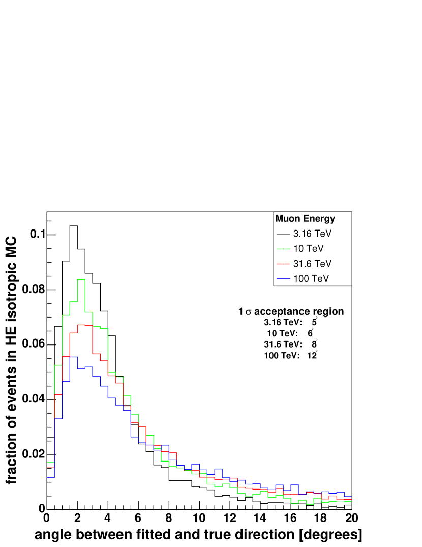
Figure 2.— Angular resolution of OD-based fit for events from the high energy isotropic MC with $>10^{5}{\rm{\;pe}}$ in the ID.

The resolution of 5–12^∘ is poor compared to the typical $1^{\circ}$ resolution of precision ID fitting algorithms, but those algorithms do not work well on these high-energy saturated events.

The efficiency of the upward-going cuts was estimated by considering all of the MC events with true values of $\cos{\Theta}<0$ and ID path length $>7{\rm{\;m}}$ and then determining the fraction of these events that pass the selection cuts described in § 3.2. This was done using isotropic MC events with $>10^{5}{\rm{\;pe}}$ since there were relatively few events in the MC with $\geq 1.75\times 10^{6}{\rm{\;pe}}$. (Above $10^{5}{\rm{\;pe}}$ the efficiency and resolution do not depend strongly on the number of ID pe deposited.) Also, as discussed in § 4.2, only the energy bins in the range $3.16-100{\rm{\;TeV}}$ were considered. The efficiency was calculated as a function of muon energy and $\cos\Theta$.

Statistical uncertainties on the efficiency determination were calculated using the Bayesian method discussed by Conway (2002). Systematic uncertainties due to uncertainties in the fitted values of the zenith angle, path length, and number of OD PMTs hit near the entry and exit points were evaluated by comparing the fitted values with the true MC values. The fitted values agree well with the MC values, and distributions of the difference between the fitted values and the MC values were used to determine an effective $1\,\sigma$ region for each parameter. The cuts on these parameters were varied by $1\,\sigma$ in either direction to determine the effect on the efficiency.

Another source of systematic uncertainty on the efficiency is prepulsing, which is not included in the MC simulation and must be estimated separately. To do this, we compared the results from the high-energy isotropic MC to a sample of 627 ultra–high-energy downward-going muon data events with $\geq 1.75\times 10^{6}{\rm{\;pe}}$ in the ID selected by a visual scan. For many of these data events, the time difference $t_{{\rm IDentry}}-t_{{\rm ODentry}}$ is negative, showing evidence of prepulsing not seen in the MC sample.

To estimate the systematic uncertainty on the efficiency calculation due to prepulsing, we calculated a heuristic correction to the MC by smearing the MC distribution of $t_{{\rm IDentry}}-t_{{\rm ODentry}}$ such that it matched the distribution of the ultra–high-energy downward-going data. We applied this adjustment to the events in the MC sample and found that an additional 1% of the MC events would be cut after accounting for prepulsing, which lengthens the negative-side error bars on the efficiency estimates by approximately 0.01.

Finally, one additional correction must be made: the efficiency has been estimated at different values for $E_{\mu}$, but the flux calculation is for the flux above a threshold energy $E_{\mu}^{\rm min}$. Since the efficiency decreases with energy, $\varepsilon\left(E_{\mu},\Theta\right)$ is an overestimate for $\varepsilon\left(\geq E_{\mu}^{\rm min},\Theta\right)$. This does not lead to a conservative upper limit for the flux, so a correction must be made. This requires knowledge of the energy spectrum of the expected signal, so we modeled the signal as an isotropic flux of neutrinos with ${d\Phi_{\nu}\left(E_{\nu}\right)}/{dE_{\nu}}\propto E_{\nu}^{-2}$ (a plausible astrophysical spectrum Gaisser 1990), used the method of § 7 to estimate the muon flux $\Phi_{\mu}\left(\geq E_{\mu}^{\rm min}\right)$, and used this muon flux to extrapolate our efficiency calculations to find $\varepsilon\left(\geq E_{\mu}^{\rm min},\Theta\right)$. This procedure yields small downward adjustments ($0.6-9\%$) to the calculated efficiency in each angular bin.

Additionally, we must also account for the efficiency of the visual scan and manual fit procedure. To do this, we did a visual scan of the 605 events from the high-energy isotropic MC with true $\cos{\Theta}<0$, true ID path length $>7{\rm{\;m}}$, and $\geq 1.75\times 10^{6}{\rm{\;pe}}$ in the ID and found that 10 of these events were eliminated in the visual scan. This gives an efficiency of roughly $98\%$, so we adjust our efficiency results by a factor of $0.98$.

The final results for the efficiency of our cuts on upward, throughgoing, $\geq 1.75\times 10^{6}{\rm{\;pe}}$ muons (including all corrections discussed above) are plotted in Figure 3.

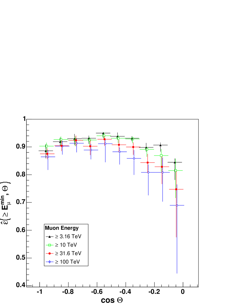
Figure 3.— Efficiency of our data reduction on upward, throughgoing, $\geq 1.75\times 10^{6}{\rm{\;pe}}$ muons as determined by the high-energy isotropic MC. Error bars include statistical and systematic errors.

4.2. Ultra–High-Energy Fraction

In order to set an upper limit on the flux of upward-going muons from cosmic neutrinos one must make an inference about the energies of the upward-going muons in the ultra–high-energy sample. Above energies of $\sim 1{\rm{\;TeV}}$, muon energy loss in water is dominated by radiative processes such as bremsstrahlung, so high-energy muons have some probability of depositing large numbers of photoelectrons in the Super-K detector and contributing to the ultra–high-energy sample. Since this energy loss is not continuous, it is not possible to estimate the muon energy for a single ultra–high-energy upward-going muon event. Rather, MC is used to make a statistical statement about the energies of the muons that make up the $\geq 1.75\times 10^{6}{\rm{\;pe}}$ sample.

The high-energy isotropic MC has been used to determine the fraction $k\left(E_{\mu}\right)$ of muons with energy $E_{\mu}$ that will deposit $\geq 1.75\times 10^{6}{\rm{\;pe}}$ in the ID, thus contributing to the ultra–high-energy sample. Results are shown in Table 2.

Table 2Fraction of high-pe events $k\left(E_{\mu}\right)$ in high energy isotropic MC

	number of MC events	$k\left(E_{\mu}\right)$
$E_{\mu}$	(out of 10000) with	(with statistical
(TeV)	$\geq 1.75\times 10^{6}{\rm{\;pe}}$ in ID	uncertainties)
0.1, 0.316, 1	0	$0.0000\begin{array}[]{c}+0.0001\\ -0.0000\end{array}$
$3.16$	35	$0.0035\pm 0.0006$
$10$	113	$0.0113\begin{array}[]{c}+0.0011\\ -0.0010\end{array}$
$31.6$	293	$0.0293\pm 0.0017$
$100$	879	$0.0879\begin{array}[]{c}+0.0029\\ -0.0028\end{array}$

Statistical uncertainties were calculated using the Bayesian method discussed by Conway (2002). As can be seen in Table 2, the three lowest energy bins — from $100\;{\rm{GeV}}$ to $1\;{\rm{TeV}}$ — do not make a significant contribution to the $\geq 1.75\times 10^{6}{\rm{\;pe}}$ sample. Hence, the rest of this analysis was done using only the four highest energy bins — from $3.16$ to $100\;{\rm{TeV}}$.

These results for $k\left(E_{\mu}\right)$ are used in § 5 to calculate the flux $\Phi_{\mu}\left(\geq E_{\mu}^{\rm min}\right)$. Since $k\left(E_{\mu}\right)$ increases with energy, it is an underestimate for $k\left(\geq E_{\mu}^{\rm min}\right)$, which leads to a conservative upper limit for $\Phi_{\mu}\left(\geq E_{\mu}^{\rm min}\right)$.

Also, since this MC only simulates the muon and not the actual neutrino interaction, the effect of lower energy debris from deep inelastic scattering events that make it into the detector has been neglected, again leading to an underestimate of $k\left(E_{\mu}\right)$. This effect is expected to be small in the energy range considered here — above $E_{\mu}=1\;{\rm{TeV}}$ at the detector entry, over 80% of the neutrino-induced upward-going muons come from over $200\;{\rm{m}}$ away from the detector, so most of the debris is absorbed by the surrounding rock, as determined using the atmospheric neutrino MC discussed in § 6.

5. Flux Calculation

The flux of upward-going muons above a threshold energy $E_{\mu}^{\rm min}$ is given by

$$\Phi_{\mu}\left(\geq E_{\mu}^{\rm min}\right)=\frac{1}{2\pi Tk\left(\geq E_{\mu}^{\rm min}\right)}{\displaystyle\sum\limits_{j=1}^{n}\frac{1}{\varepsilon\left(\geq E_{\mu}^{\rm min},\Theta_{j}\right)A\left(\Theta_{j}\right)}},$$ (1)

where $n$ is the total number of upward-going muon events observed and $\Theta_{j}$ is the zenith angle of the $j$th event. The efficiency $\varepsilon\left(\geq E_{\mu}^{\rm min},\Theta_{j}\right)$ and the ultra–high-energy fraction $k\left(\geq E_{\mu}^{\rm min}\right)$ are calculated in § 4. $T$ is the detector livetime, which is 1679.6 days for SK-I. $A\left(\Theta_{j}\right)$ is the effective area of the Super-K detector perpendicular to the direction of incidence for tracks with a path length of $>7{\rm{\;m}}$ in the ID. The average effective area of the detector is $\sim 1200{\rm{\;m}}^{2}$.

Equation (1) has been applied to the detected upward-going muon event discussed in § 3.2 to calculate $\Phi_{\mu}\left(\geq E_{\mu}^{\rm min}\right)$ for $E_{\mu}^{\rm min}$ in the range $3.16-100{\rm{\;TeV}}$. Results are shown in Table 3.

Table 3The flux of ultra-high energy upward-going muons as observed by SK-I.

$E_{\mu}^{\rm min}$	$\Phi_{\mu}\left(\geq E_{\mu}^{\rm min}\right)$
(TeV)	(${\rm{cm^{-2}s^{-1}sr^{-1}}}$)
$3.16$	$2.64\times 10^{-14}\begin{array}[]{c}+16.1\%\\ -17.9\%\end{array}$
$10$	$8.23\times 10^{-15}\begin{array}[]{c}+9.48\%\\ -9.73\%\end{array}$
$31.6$	$3.25\times 10^{-15}\begin{array}[]{c}+6.67\%\\ -6.40\%\end{array}$
$100$	$1.10\times 10^{-15}\begin{array}[]{c}+4.96\%\\ -4.09\%\end{array}$

Systematic uncertainties include a $0.1\%$ uncertainty on the live time $T$, a $0.3\%$ uncertainty on the effective area $A$, the total efficiency uncertainties shown in Figure 3, and the statistical uncertainties on $k$ shown in Table 2. This flux includes both the potential signal from astrophysical neutrinos and a background of atmospheric neutrinos.

6. Expected Atmospheric Background from Monte Carlo

When searching for neutrinos from astrophysical sources, the dominant background is the atmospheric neutrino spectrum. Atmospheric neutrinos are produced by decays of pions and kaons formed when cosmic rays interact with particles in the atmosphere. We have used an atmospheric neutrino MC that is a 100 yr equivalent sample of events due to the atmospheric neutrino flux. The neutrino flux in Honda et al. (2004) was used up to neutrino energies of 1 TeV. At 1 TeV, the calculated flux in Volkova (1980) was rescaled to the Honda et al. flux. Above 1 TeV, the rescaled flux from Volkova was used up to 100 TeV. Neutrino interactions were modeled using the GRV94 parton distribution functions (Gluck et al. 1995), and muon propagation through the rock and water was modeled using GEANT. Further details on the atmospheric neutrino MC can be found in Ashie et al. (2005). No correction is made for neutrino oscillations, because based on the oscillation parameters determined in Ashie et al. (2005), the neutrino oscillation probability is negligible for neutrinos above $1{\rm{\;TeV}}$.

This atmospheric MC is split into two parts: a partially-contained/fully-contained (PC/FC) sample, which consists of events with neutrino interaction points inside the ID plus a shell 50 cm thick surrounding the ID (the insensitive region), and an upward-going muon sample, which consists of events with neutrino interaction points outside the ID. Note that these two samples overlap because they both cover the 50 cm insensitive region.

The OD-based fit was applied to the events in the atmospheric MC, using the same cuts that were applied to the SK-I data. A total of 11 MC events passed the $\geq 1.75\times 10^{6}{\rm{\;pe}}$, $\cos{\Theta}\leq 0.1$, path length $>7{\rm{\;m}}$, $N_{{\rm ODentry}}$ and $N_{{\rm ODexit}}\geq 10$, OD/ID timing, and manual fit cuts. Out of these 11, 2 are from the PC/FC sample, both with interaction points inside the ID. The remaining 9 events are from the upward-going muon sample: 3 events with interaction points in the 50 cm insensitive region, 1 event in the water of the OD, and 5 events in the rock surrounding the detector.

All of these background events are deep inelastic scattering (DIS) events where an interaction between a muon neutrino and a nucleon produces a muon plus a spray of lower energy particles. The 6 events with interaction points within the detector (ID or OD) have muon energies of $0.1-0.8{\rm{\;TeV}}$, and the 5 events occurring in the rock have muon energies of $1-20{\rm{\;TeV}}$. This difference in the energy range can be understood as follows: For DIS events occurring a long distance ($>2{\rm{\;m}}$ or so) from the detector, only the muon will reach the detector since the lower energy debris will be absorbed by the surrounding rock, but for nearby events or events occurring in the water of the OD, some of these lower energy particles will enter the detector as well. This means that nearby events can be included in the $\geq 1.75\times 10^{6}{\rm{\;pe}}$ sample with lower muon energies than more distant events.

Since the insensitive region is covered by both the PC/FC and the upward-going muon MC samples, we divided the 3 events originating from this region in half, for a total of 1.5 events in the insensitive region. This gives a total of 9.5 MC events in 100 yr of simulated live time. Scaling the 100 yr MC to SK-I’s live time of 1679.6 days gives an expected background of $0.44$ events due to atmospheric neutrinos during the operation of SK-I.

The statistical uncertainty in this background measurement of the MC events is 31%. There are also significant systematic uncertainties: the normalization of the atmospheric neutrino flux has a theoretical uncertainty of $\pm 10\%$ at neutrino energies below $10{\rm{\;GeV}}$ (Ashie et al. 2005). In order to extend this to the energy range of the expected background, we must also account for the uncertainty of 0.05 in the spectral index of the primary cosmic ray spectrum above 100 GeV, which leads to a 0.05 uncertainty in the spectral index for atmospheric neutrinos above $10{\rm{\;GeV}}$ (Ashie et al. 2005).

To determine how much this uncertainty affects our result for the background, we consider the atmospheric neutrino flux to be known at $10{\rm{\;GeV}}$, and we calculate the uncertainty of the total flux $\Phi_{\nu}$ above a threshold energy $10.6{\rm{\;TeV}}$, the average neutrino energy of the atmospheric MC events passing our cuts. For a differential flux of ${d\Phi_{\nu}}/{dE_{\nu}}\propto E_{\nu}^{-\gamma}$ with $\gamma=3.7\pm 0.05$, the spectral index uncertainty gives us a $\pm 37\%$ uncertainty on the atmospheric neutrino flux $\Phi_{\nu}$.

Finally, the neutrino cross-section at high energies is thought to be known to within $10\%$ or less, so we include an additional $10\%$ uncertainty to account for this. These uncertainties are summarized in Table 4 and lead to a total uncertainty on the background of $50\%$.

Table 4Systematic uncertainties in atmospheric neutrino background

Source of Uncertainty	Uncertainty
Statistical	31%
Absolute normalization of atm $\nu$ flux	10%
Primary spectral index	37%
Neutrino cross-section uncertainty	10%
Total uncertainty in background flux	50%

Other potential errors (uncertainties in the simulation of the SK detector and varying hadron multiplicities in different deep inelastic scattering models) were tested and shown to not make a significant contribution to the systematic uncertainty.

Another potential background source of high-energy neutrinos not included in the 100 yr atmospheric MC is the prompt atmospheric neutrino flux, which arises from decays of short-lived charmed particles produced when cosmic rays interact with particles in the atmosphere. This flux is not as well-understood as the conventional atmospheric neutrino flux from decays of pions and kaons, but it is expected to have a harder spectrum and therefore is expected to become more important as we push towards higher energy scales.

Based on the 100 yr atmospheric MC, we calculate an expected background for this analysis of $0.44\pm 0.22$ events, compared to the 1 event observed. However, there are three effects that this MC does not take into account: it does not include neutrinos over $100{\rm{\;TeV}}$, it does not include the prompt atmospheric neutrino flux, and it does not account for attenuation of neutrinos passing through the Earth. We account for these issues by making corrections based on an analytical calculation discussed in § 7.

Also, it is important to note that the atmospheric background — both conventional and prompt — comes from a lower energy range than that for which we expect to observe the possible signal of neutrinos from astrophysical sources. Roughly speaking, the peak 90% of the expected upward-going muon events come from muons with energies in the range $E_{\mu}=0.02-10{\rm\;TeV}$ for conventional atmospheric neutrinos, and $E_{\mu}=0.2-200{\rm\;TeV}$ for prompt neutrinos. As we learned from the 11 background events in the 100 yr atmospheric MC, muons with energies $E_{\mu}<1{\rm\;TeV}$ contribute to the $1.75\times 10^{6}{\rm{\;pe}}$ sample mainly via debris from DIS events very close to the detector rather than from catastrophic energy loss of the muon.

Since there are many more low-energy events in the atmospheric spectrum, they will dominate even though each one only has a tiny probability of depositing a large amount of energy in the detector. In contrast, the peak 90% of the expected muon events from a harder spectrum — a hypothetical $E_{\nu}^{-2}$ astrophysical flux — come from the range $E_{\mu}=7-6000{\rm\;TeV}$. Thus, even though the atmospheric flux is very small in the energy range $E_{\mu}=3-100{\rm\;TeV}$ and above where we are setting our limit, the high-pe tails of the distribution from lower energy events dominate our background simply because of the much larger flux of lower energy atmospheric events.

7. Analytical Estimate of Expected Muon Flux

7.1. Method for Calculating Muon Flux

In order to better understand our observed flux of high-energy upward-going muons, we developed a method to calculate the expected upward-going muon event rate due to a predicted flux of neutrinos. We have used this to plot curves for theoretical muon fluxes in Figure 5 and also to adjust the atmospheric background calculated with MC in § 6 by correcting for effects not included in the simulation.

To convert a model neutrino flux into an expected upward-going muon event rate, we follow the calculation detailed in Gaisser et al. (1995) and Gandhi et al. (1996). The flux of muons $\Phi_{\mu}\left(\geq E_{\mu}^{\rm min}\right)$ above an energy threshold $E_{\mu}^{\rm min}$ is given by

$$\Phi_{\mu}\left(\geq E_{\mu}^{\rm min}\right)=\int_{E_{\mu}^{\rm min}}^{\infty}dE_{\nu}P_{\mu}\left(E_{\nu},\,E_{\mu}^{\rm min}\right)\frac{d\Phi_{\nu}^{\rm av}\left(E_{\nu}\right)}{dE_{\nu}},$$ (2)

where $P_{\mu}\left(E_{\nu},\,E_{\mu}^{\rm min}\right)$ is the probability that an incoming neutrino with energy $E_{\nu}$ will produce a muon with energy above the threshold $E_{\mu}^{\rm min}$ at the detector, and ${d\Phi_{\nu}^{\rm av}\left(E_{\nu}\right)}/{dE_{\nu}}$ is the differential neutrino flux averaged over solid angle and reduced by an exponential factor due to attenuation of the neutrinos as they pass through the Earth.

$P_{\mu}\left(E_{\nu},\,E_{\mu}^{\rm min}\right)$ depends on both the charged-current neutrino cross-section and the energy lost by the resulting muon as it propagates through the Earth. In our calculation, we calculate the cross-section using the GRV94 parton distribution functions (Gluck et al. 1995) applied with the code used in Gandhi et al. (1996) provided by M. Reno (2005, private communication), and we use an effective muon range calculated using MC methods (Lipari & Stanev 1991).

As discussed in Gandhi et al. (1996), the appropriate cross-section $\sigma\left(E_{\nu}\right)$ to use in the neutrino attenuation factor lies between the charged current cross section and the sum of the charged and neutral current cross sections, so we have calculated the flux with the upper and lower limits and averaged the resulting fluxes together.

We integrated equation (2) numerically using various predicted models of the neutrino flux ${d\Phi_{\nu}}/{dE_{\nu}}$ to calculate theoretical $\Phi_{\mu}\left(\geq E_{\mu}^{\rm min}\right)$ curves. These are shown in Figure 5 for comparison to our experimental limits.

7.2. Analytical Estimate of Expected Background

Of particular interest here are the model fluxes of the background due to atmospheric neutrinos, both conventional and prompt. We use the method discussed in § 7.1 to correct for the omissions in the 100 yr atmospheric MC discussed in § 6 by accounting for neutrinos over $100{\rm{\;TeV}}$, attenuation of neutrinos in the Earth, and the flux of prompt neutrinos.

The expected number of events $N$ seen by Super-K in livetime $T$ is given by

$$N=2\pi TA_{\rm av}\int_{0}^{\infty}dE_{\mu}^{\rm min}\frac{d\Phi_{\mu}\left(\geq E_{\mu}^{\rm min}\right)}{dE_{\mu}^{\rm min}}k\left(E_{\mu}^{\rm min}\right),$$ (3)

where ${d\Phi_{\mu}\left(\geq E_{\mu}^{\rm min}\right)}/{dE_{\mu}^{\rm min}}$ is the derivative of the curve calculated by the method in § 7.1 and $k\left(E_{\mu}^{\rm min}\right)$ is the fraction of muons with energy above $E_{\mu}^{\rm min}$ that will deposit $\geq 1.75\times 10^{6}{\rm{\;pe}}$ in the ID. We estimated $k\left(E_{\mu}^{\rm min}\right)$ using the results of the high-energy isotropic MC discussed in § 4.2 by fitting the data in Table 2 with a simple power law with a cutoff at 1 since $k$ represents a probability. Figure 4 compares this power-law fit to results from 100 yr atmospheric MC, illustrating that the power law is reasonable in the energy range we are considering.

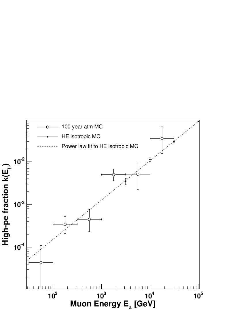
Figure 4.— Fraction of events $k\left(E_{\mu}\right)$ that deposit $\geq 1.75\times 10^{6}{\rm{\;pe}}$ in the ID for the 100 yr atmospheric MC (open circles), the high-energy isotropic MC (filled squares), and a power-law fit to the results from high-energy isotropic MC. The power law is a reasonable approximation for the dominant energy range of the atmospheric flux ($E_{\mu}=100{\rm\;GeV}-30{\rm\;TeV}$).

We analytically estimated the expected number of events in the 100 yr atmospheric MC by starting with the same input neutrino flux, applying equation (2) without the exponential neutrino attenuation factor and integrating up to a maximum neutrino energy of $E_{\nu}^{\rm max}=100{\rm\;TeV}$. We then used this muon flux in equation (3) to find the expected number of background events in 100 yr and obtained $N_{100}=7.39$ expected events. (The 100 subscript denotes 100 yr of exposure.) This matches our results from the 100 yr atmospheric MC to within statistical uncertainties.

To estimate the effects of neutrinos above 100 TeV, we repeated the above calcuation without the $E_{\nu}^{\rm max}=100{\rm\;TeV}$ cutoff and obtained $N_{100}=7.47{\rm\;events}$, an increase of $1.1\%$. Including the neutrino attenuation factor as well, we obtained $N_{100}=7.29\pm 0.02{\rm\;events}$ per 100 yr of exposure, a decrease of $2.4\%\pm 0.3\%$. (The uncertainty is due to the choice of cross-section.)

We also used this calculation to correct for the prompt atmospheric neutrino flux. To account for the theoretical uncertainty in the prompt flux due to differences between various flux models, we defined a high model and a low model for the prompt flux that bracket the models shown in Figure 1 of Gelmini et al. (2003) that are not ruled out by experimental limits. The models used are discussed in more detail in Thunman et al. (1996), Zas et al. (1993), Ryazhskaya et al. (2002), Bugaev et al. (1989), Pasquali et al. (1999), and Gelmini et al. (2000a, b). Our analytical calculation gives $N_{100}=0.033{\rm\;events}$ for the low model and $N_{100}=0.94{\rm\;events}$ for the high model, corresponding to a prompt flux that is $6.7\%\pm 6.2\%$ of the flux of conventional atmospheric neutrinos.

Based on these results, we correct the background estimate made using the 100 yr atmospheric MC in § 6 by applying these relative scalings to the result of $0.44{\rm\;events}$ in the SK-I livetime from § 6. This gives us a final result for the background of $0.46\pm 0.23{\rm\;events}$ for the SK-I exposure.

8. Upper Limit for Muon Flux from Cosmic Neutrinos

Using the observed ultra–high-energy upward-going muon signal of 1 event and the expected atmospheric neutrino background of $0.46\pm 0.23$ events, we have calculated $90\%$ confidence upper limits for the upward-going muon flux in the $3.16-100{\rm{\;TeV}}$ range due to neutrinos from astrophysical sources (or any other non-atmospheric sources).

This was done using the method of Feldman & Cousins (1998), with the systematic uncertainties incorporated using the method of Cousins & Highland (1992), as implemented by Conrad et al. (2003) and improved by Hill (2003). This method incorporates both uncertainties in the background flux and uncertainties in the flux factor $f$ relating the observed number of events $n$ to the observed flux $\Phi$: $\Phi=f\,n$. The uncertainty in $f$ includes systematic errors in the livetime, effective area, efficiency, and ultra–high-energy fraction. For the confidence interval calculation, the largest percent error for each energy bin from Table 3 was used as the percent uncertainty in $f$. The uncertainties in both the background and the flux factor were assumed to have a Gaussian distribution.

The final results are shown in Table 5 and plotted in Figure 5, along with models of various possible signals from AGNs (Stecker & Salamon 1996; Mannheim et al. 2001) and GRBs (Waxman & Bahcall 1999), as well as the backgrounds due to atmospheric neutrinos (Honda et al. 2004; Volkova 1980) and prompt neutrinos (Gelmini et al. 2003).

Table 5Confidence intervals for the upward-going muon flux due to neutrinos from astrophysical sources.

$E_{\mu}^{\rm min}$	90% C.L. range
(TeV)	(${\rm{\;cm^{-2}s^{-1}sr^{-1}}}$)
$3.16$	$0-1.03\times 10^{-13}$
$10$	$0-3.19\times 10^{-14}$
$31.6$	$0-1.26\times 10^{-14}$
$100$	$0-4.28\times 10^{-15}$

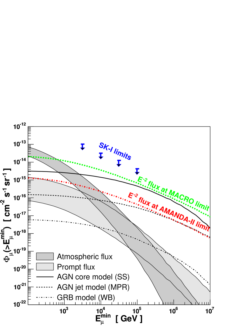
Figure 5.— Upper limits from this analysis on muon $\left(\mu^{+}+\mu^{-}\right)$ flux above energy threshold $E_{\mu}^{\rm min}$, compared to various model fluxes. Models shown for muon flux due to astrophysical neutrinos are AGN models from SS (Stecker & Salamon 1996) and MPR (Mannheim et al. 2001), and a GRB model from WB (Waxman & Bahcall 1999). Also shown is the atmospheric background, as modeled by Honda et al. (2004) below $E_{\nu}=1{\;{\rm TeV}}$ and by Volkova (1980) rescaled to match the Honda model above $E_{\nu}=1{\;{\rm TeV}}$. The upper edge of the atmospheric band represents the horizontal flux, and the lower edge represents the vertical flux. The background due to muons from prompt atmospheric neutrinos (assumed to be isotropic) is shown for a range of possible models as summarized in Gelmini et al. (2003). Finally, we also show the expected muon flux from a model neutrino flux that is isotropic and proportional to $E_{\nu}^{-2}$ at the values of the limit set by MACRO (Ambrosio et al. 2003) and AMANDA-II (Groß et al. 2005). The models of the neutrino flux have been converted to a muon flux with equation (2) using the GRV94 parton distributions (Gluck et al. 1995) and the effective muon range from Lipari & Stanev (1991).

The upper limits calculated here are consistent with the models of astrophysical signals. Also shown are models with a hypothetical isotropic neutrino flux with a spectrum proportional to $E_{\nu}^{-2}$ and a normalization scaled to the limits on an $E_{\nu}^{-2}$ flux set by MACRO (Ambrosio et al. 2003) and AMANDA-II (Groß et al. 2005). The model neutrino fluxes were converted into muon fluxes using equation (2) as discussed in § 7.

To facilitate easier comparison with other experiments, we also convert our limits on the muon flux into approximate limits on the neutrino flux. In order to do this, we assume a model neutrino flux that is isotropic and proportional to $E_{\nu}^{-2}$. To get an approximate neutrino limit, we find normalization factors for an $E_{\nu}^{-2}$ muon flux curve such that the curve passes through each of our four limit points in Figure 5, and we use these factors to find the implied limits on $E_{\nu}^{-2}$ flux.

In order to determine the approximate neutrino energy range in which these limits are valid, we use equation (2) to determine the neutrino energy range that produces the bulk of the muon signal for a given value of the muon energy threshold $E_{\mu}^{\rm min}$. We define the energy range as the range that (1) produces 90% of the muon flux above $E_{\mu}^{\rm min}$ and (2) has a higher value of the integrand of equation (2) within the range than anywhere outside the range. This definition is based on the definition of highest posterior density intervals as described by Conway (2002).

The results of these approximations for neutrino limits and energy ranges are shown in Table 6

Table 6Approximate upper limits from SK-I on astrophysical neutrinos $\left(\nu_{\mu}+\bar{\nu}_{\mu}\right)$.

$E_{\mu}^{\rm min}$	90% C.L. upper limit	Neutrino energy range
(TeV)	(${\rm{GeV\,cm^{-2}s^{-1}sr^{-1}}}$)	(GeV)
$3.16$	$6.0\times 10^{-5}$	$6.3\times 10^{3}-1.4\times 10^{6}$
$10$	$3.7\times 10^{-5}$	$1.7\times 10^{4}-2.4\times 10^{6}$
$31.6$	$3.2\times 10^{-5}$	$4.7\times 10^{4}-5.1\times 10^{6}$
$100$	$2.6\times 10^{-5}$	$1.4\times 10^{5}-1.1\times 10^{7}$

and are also plotted in Figure 6,

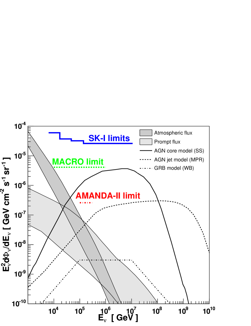
Figure 6.— Approximate upper limits from SK-I on astrophysical neutrinos $\left(\nu_{\mu}+\bar{\nu}_{\mu}\right)$. Models shown are the same as in Figure 5. Note that converting from a muon flux limit to a neutrino flux limit requires additional assumptions - our limits on the muon flux are shown in Figure 5.

with the same models and experimental limits as shown in Figure 5. To draw our limits on this plot, we chose to draw only the most sensitive limit in each energy range.

Note that these results for the limits on the neutrino flux are only approximations made to facilitate comparison to other experiments — our primary results are the limits on the muon flux shown in Table 5 and Figure 5.

9. Conclusions

In conclusion, we have developed a method for analyzing Super-K’s highest energy data to search for evidence of high-energy neutrino flux from astrophysical sources. We have done a thorough study of the efficiency and the expected backgrounds from this method and applied our method to the SK-I data sample. Our study of the highest energy events in SK-I does not show evidence of a high-energy cosmic neutrino signal.

We have set upper limits on the muon flux due to cosmic neutrino sources. These limits are consistent with the results of other experiments (Ambrosio et al. 2003; Groß et al. 2005). It is possible that an astrophysical neutrino signal could be within the grasp of the next generation of neutrino detectors such as IceCube (Ahrens et al. 2004) and ANTARES (Katz 2004).

10. Acknowledgments

We gratefully acknowledge the cooperation of the Kamioka Mining and Smelting Company. The Super-Kamiokande experiment has been built and operated from funding by the Japanese Ministry of Education, Culture, Sports, Science and Technology, the United States Department of Energy, and the US National Science Foundation. Some of us have been supported by funds from the Korean Research Foundation (BK21) and the Korea Science and Engineering Foundation, the Polish Committee for Scientific Research (grant 1P03B08227), Japan Society for the Promotion of Science, and Research Corporation’s Cottrell College Science Award.

References

- Abe et al. (2006) Abe, K. et al. 2006, ApJ, 652, 198
- Ahrens et al. (2004) Ahrens, J. et al. 2004, Astropart. Phys., 20, 507
- Ambrosio et al. (2003) Ambrosio, M. et al. 2003, Astropart. Phys., 19, 1
- Ashie et al. (2005) Ashie, Y. et al. 2005, Phys. Rev. D, 71, 112005
- Bottai & Perrone (2001) Bottai, S. & Perrone, L. 2001, Nucl. Instrum. Methods Phys. Res., Sect. A, 459, 319
- Bugaev et al. (1989) Bugaev, E. V., Naumov, V. A., Sinegovskii, S. I., & Zaslavskaia, E. S. 1989, Nuovo Cimento C, 12, 41
- Conrad et al. (2003) Conrad, J., Botner, O., Hallgren, A., & Pérez de Los Heros, C. 2003, Phys. Rev. D, 67, 012002
- Conway (2002) Conway, J. 2002, Efficiency Uncertainties: A Bayesian Prescription, Tech. Rep. CDF/PUB/5894, CDF, Batavia, IL, http://www-cdf.fnal.gov/physics/statistics/statistics_recommendations.html
- Cousins & Highland (1992) Cousins, R. D. & Highland, V. L. 1992, Nucl. Instrum. Methods Phys. Res., Sect. A, 320, 331
- Desai et al. (2003) Desai, S. et al. 2003, in Proc. 28th Intl. Cosmic Ray Conf., ed. T. Kajita et al., Trukuba, 1673
- Desai et al. (2004) Desai, S. et al. 2004, Phys. Rev. D, 70, 083523
- Feldman & Cousins (1998) Feldman, G. J. & Cousins, R. D. 1998, Phys. Rev. D, 57, 3873
- Fukuda et al. (2003) Fukuda, S. et al. 2003, Nucl. Instrum. Methods Phys. Res., Sect. A, 501, 418
- Fukuda et al. (1999) Fukuda, Y. et al. 1999, Phys. Rev. Lett., 82, 2644
- Gaisser (1990) Gaisser, T. K. 1990, Cosmic rays and particle physics (Cambridge and New York, Cambridge University Press, 1990, 292 p.)
- Gaisser et al. (1995) Gaisser, T. K., Halzen, F., & Stanev, T. 1995, Phys. Rep., 258, 173
- Gandhi et al. (1996) Gandhi, R., Quigg, C., Reno, M. H., & Sarcevic, I. 1996, Astropart. Phys., 5, 81
- Gelmini et al. (2000a) Gelmini, G., Gondolo, P., & Varieschi, G. 2000a, Phys. Rev. D, 61, 056011
- Gelmini et al. (2000b) —. 2000b, Phys. Rev. D, 61, 036005
- Gelmini et al. (2003) —. 2003, Phys. Rev. D, 67, 017301
- Gluck et al. (1995) Gluck, M., Reya, E., & Vogt, A. 1995, Z. Phys., C, 67, 433
- Groß et al. (2005) Groß, A. et al. 2005, preprint (astro-ph/0505278)
- Halzen & Hooper (2002) Halzen, F. & Hooper, D. 2002, Reports of Progress in Physics, 65, 1025
- Hill (2003) Hill, G. C. 2003, Phys. Rev. D, 67, 118101
- Honda et al. (2004) Honda, M., Kajita, T., Kasahara, K., & Midorikawa, S. 2004, Phys. Rev. D, 70, 043008
- Katz (2004) Katz, U. F. 2004, Eur. Phys. J. C, 33, 971
- Lipari & Stanev (1991) Lipari, P. & Stanev, T. 1991, Phys. Rev. D, 44, 3543
- Mannheim et al. (2001) Mannheim, K., Protheroe, R. J., & Rachen, J. P. 2001, Phys. Rev. D, 63, 023003
- Pasquali et al. (1999) Pasquali, L., Reno, M. H., & Sarcevic, I. 1999, Phys. Rev. D, 59, 034020
- Ryazhskaya et al. (2002) Ryazhskaya, O. G., Volkova, L. V., & Saavedra, O. 2002, Nucl. Phys. Proc. Suppl., 110, 531
- Staśto (2004) Staśto, A. M. 2004, Int. J. Mod. Phys. A, 19, 317
- Stecker & Salamon (1996) Stecker, F. W. & Salamon, M. H. 1996, Space Sci. Rev., 75, 341
- Thunman et al. (1996) Thunman, M., Ingelman, G., & Gondolo, P. 1996, Astropart. Phys., 5, 309
- Volkova (1980) Volkova, L. V. 1980, Sov. J. Nucl. Phys., 31, 784
- Waxman & Bahcall (1999) Waxman, E. & Bahcall, J. 1999, Phys. Rev. D, 59, 023002
- Zas et al. (1993) Zas, E., Halzen, F., & Vázquez, R. A. 1993, Astropart. Phys., 1, 297