Imaging extended sources with coded mask telescopes: Application to the INTEGRAL IBIS/ISGRI instrument

Abstract

Context. In coded mask techniques, reconstructed sky images are pseudo-images: they are maps of the correlation between the image recorded on a detector and an array derived from the coded mask pattern.

Aims. The INTEGRAL/IBIS telescope provides images where the flux of each detected source is given by the height of the local peak in the correlation map. As such, it cannot provide an estimate of the flux of an extended source. What is needed is intensity sky images giving the flux per solide angle as typically done at other wavelengths.

Methods. In this paper, we present the response of the INTEGRAL IBIS/ISGRI coded mask instrument to extended sources. We develop a general method based on analytical calculations in order to measure the intensity and the associated error of any celestial source and validated with Monte-Carlo simulations.

Results. We find that the sensitivity degrades almost linearly with the source extent. Analytical formulae are given as well as an easy-to-use recipe for the INTEGRAL user. We check this method on IBIS/ISGRI data but these results are general and applicable to any coded mask telescope.

1 Introduction

The usual techniques of imaging the sky by focusing the radiation become ineffective above $\sim$ 15 $\mathrm{keV}$ due to technological constraints. Future observatories (e.g. Constellation-X/HXT, Hailey et al. 2004 ; Simbol-X, Ferrando et al. 2005) will push this limit up to 60-70 $\mathrm{keV}$ with the use of multi-layer grazing optics Ramsey et al. (2002). Collimators using the standard on/off techniques are limited by the source density at low energies (¡ 50 $\mathrm{keV}$) and by the internal background variability at higher energies. Both problems are addressed with coded-aperture techniques, which have been employed successfully in high-energy astronomy in several previous missions such as the GRANAT/SIGMA instrument Paul et al. (1991) or the BeppoSAX Wide Field Cameras Jager et al. (1997). In such telescopes, source radiation is spatially modulated by a mask consisting of an array of opaque and transparent elements and recorded by a position sensitive detector, allowing simultaneous measurement of source plus background in the detector area corresponding to the mask holes and background only in that corresponding to the opaque elements. For each point source in the field of view the two-dimensional distribution of events projected onto the detector reproduces a unique shadow of the mask pattern and the recorded shadowgram is the sum of many such distributions. The popular way to reconstruct the sky image is based on a correlation procedure between the recorded image and a decoding array derived from the spatial characteristics of the mask pattern. One can describe the usual properties of telescopes for these systems as follows: the angular resolution, defined by the angle subtended by the smallest mask element seen from the detector, and the field of view (FOV) divided in two parts: the Fully Coded Field of View (FCFOV) representing the sky region where the recorded source radiation is fully modulated by the mask and the Partially Coded Field of View (PCFOV) the region where a source projects only a part of the mask pattern on the detector.

Many mask patterns have been designed and employed in the past for optimizing the imaging quality of point-like sources in the high-energy domain. Recently, Schäfer (2004) has presented a novel method for imaging extended sources by constructing mask patterns with a pre-defined Point Spread Function (PSF). In this paper, we have developed a method to reconstruct the intensity and estimate the corresponding error of extended sources seen through a given coded mask telescope. This work is motivated by the fact that several sources of interest in $\gamma$-ray astronomy must be considered as extended in order to properly derive their intensity such as supernova remnants (hereafter, SNRs): the Tycho SNR (with an apparent diameter $\theta$ of $\sim$ 8^′), SN 1006 ($\theta\sim$ 30^′), G 347.3-0.5 ($\theta\sim$ 1^∘) or RX J0852-4622 ($\theta\sim$ 2^∘), clusters of galaxies (e.g. Coma Cluster, $\theta\sim 1^{\circ}$), and diffuse interstellar emission from various high-energy processes. We have applied this method to the IBIS/ISGRI instrument onboard the INTEGRAL satellite but the results presented here could be easily adapted to any coded mask telescope. We briefly describe the basic properties of IBIS and the principles of the standard data analysis we used for simulating celestial extended sources in section 2, considering the simplest case of a uniform disk. We present our results concerning the IBIS response for this source geometry over a large range of radii (section 3.1) as well as in an astrophysical case: the supernova remnant SN 1006 (section 3.2). These results allow us to find a general method to reconstruct the flux and the associated error of an extended source presented in sections 4.1 and 4.3, respectively. We also describe the tests we performed on the Crab Nebula and compare the results of this method to those of the standard analysis (section 4.2). In a joint paper, we have successfully applied this method on the IBIS/ISGRI data of the Coma Cluster Renaud et al. (2006), the first extended source detected with IBIS. Finally, we give practical tips on the use of this method for any interested observer.

2 Imaging sources with a coded mask telescope

2.1 General imaging procedure

In coded aperture imaging systems, a mask consists in an array M of 1 (transparent) and 0 (opaque) elements. The detector array D (the real image) is simply the convolution of the sky image S with M plus an unmodulated background array B. If there exists an inverse correlation array G such that (M$\star$G)${}_{ij}=\delta_{ij}$, then the reconstructed sky image is given by the following operation Fenimore & Cannon (1981):

$$S^{\prime}=D\star G=S\star M\star G+B\star G=S+B\star G$$ (1)

In the case where the mask M is derived from a cyclic replication of the same basic pattern and the background B is given by a flat array then the term B$\star$G is constant and can be removed. The quality of the object reconstruction therefore depends on the choice of M and G Caroli et al. (1987). Fenimore & Cannon (1978) have found mask patterns with such properties, including the Modified Uniformly Redundant Arrays (hereafter, MURAs). These coded masks are nearly-optimum and possess a correlation inverse matrix by setting G = 2M - 1. For those systems the resulting sky image of a single point-like source in the FCFOV will have a main peak at the source position of roughly the size of one projected mask element, with flat sidelobes in the FCFOV (for a perfect detector) and 8 main source ghosts in the PCFOV.

2.2 IBIS properties

We consider the IBIS telescope Ubertini et al. (2003) launched onboard the ESA $\gamma$-ray space mission INTEGRAL Winkler et al. (2003) on October 2002. The IBIS coded mask imaging system includes a replicated MURA (see section 2.1) mask Gottesman & Fenimore (1989) of tungsten elements and 2 pixellated $\gamma$-ray detectors: ISGRI Lebrun et al. (2003), the low-energy camera (15 $\mathrm{keV}$ - 1 $\mathrm{MeV}$) and PICsIT, operating between 175 $\mathrm{keV}$ and 10 $\mathrm{MeV}$ Labanti et al. (2003). We focus here on IBIS/ISGRI but the results can be adapted to any coded mask imaging system. The physical characteristics of the IBIS telescope define a FCFOV of 8.3${}^{\circ}\times$ 8.3^∘ and a total FOV of 29^∘ $\times$ 29^∘ at zero sensitivity. The nominal angular resolution is 12^′ (FWHM) and standard ISGRI images are sampled every $\sim 5$^′ , which is the angular size of detector pixels seen from the mask, allowing fine imaging and positioning of detected celestial sources. The decoding array G is oversampled at the pixel scale in order to optimize the signal to noise ratio of point-like sources in the reconstructed image. One may refer to the papers of Gros et al. (2003) and Goldwurm et al. (2003) for details on the shape of the System Point Spread Function (hereafter, SPSF) and the full description of the implemented algorithm for IBIS data, respectively. Goldwurm et al. (2003) show a variation of finely balanced cross correlation Fenimore & Cannon (1981) generalized to the total (FC+PC)FOV.

2.3 Imaging extended sources

In the following, any extended source will be considered as a large number of unresolved points. The principle of our method for imaging extended sources is as follows: first, we have calculated the fraction of pixel area covered by a given projected mask element (called Pixel Illumation Factor, PIF) corresponding to each point-like source given its relative sky position. These calculations take into account all the instrumental features of IBIS such as efficiency, dead zones between pixels and detector modules of ISGRI, mask thickness and transparencies of all the intervening materials in the ISGRI energy range (15 $\mathrm{keV}$ – 1 $\mathrm{MeV}$). Second, we have performed a weighted sum of each of the point-like source contributions to obtain the shadowgram of any extended sky source according to the following equation:

$$D_{kl}=\sum_{w=1}^{N}f_{w}\times{PIF_{kl}^{w}}$$ (2)

where D_kl is the image recorded on ISGRI, N refers to the number of unresolved points forming the extended source, and f_w represents the flux of each point source (w) with $\sum{f_{w}}=F$, the total flux of the extended source.

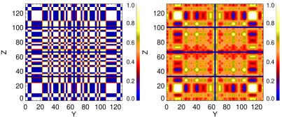
Figure 1: The recorded ISGRI shadowgram of the PIF values for an on-axis point-like source (left) and that of a uniform disk of $\sim 20$^′ radius (right) without background. Dead zones between modules and mask elements are clearly visible.

In order to illustrate the blurring effect due to the source extent, Figure 1 shows the ISGRI shadowgram of PIF values corresponding to an on-axis point-like source and that of a uniform disk of $\sim$ 20^′ radius. The overall pattern of the PIF shadowgram has a very little dependence on energy and only the relative amplitude of fluctuations depends on the energy. Finally, in order to reconstruct the sky images, we have used the standard deconvolution included in the Off-Line Scientific Analysis Goldwurm et al. (2003), version 5.0. We decided to perform these simulations in connection with what an observer can expect by analyzing IBIS/ISGRI data of any celestial region. We have chosen to simulate a disk as discussed in section 1, assuming that each individual point source contribution forming the extended source emit the same flux (i.e. the factor f_w in the equation 2 is constant, each extended source is uniform). We have distinguished two different relative positions in the sky: an on-axis source and one in the PCFOV, 9^∘ away from the telescope axis, i.e. where the IBIS sensitivity is reduced by a factor of almost 2.

3 Sensitivity to extended sources

Simulations were performed for several radii, from 0 (i.e. , a point-like source) to $\sim$ 1^∘ keeping constant the total flux F equal to $\sum_{w=1}^{N}f_{w}$. One should notice that in the standard reconstructed images, the flux of point-like sources in the FOV is given by the peak of their associated SPSF after fitting with a two-dimensional gaussian (see Gros et al. 2003). Therefore, for each reconstructed sky image, we have measured the maximal pixel flux within the apparent diameter of each extended source (hereafter, f_max) to estimate the IBIS/ISGRI response to the global peak reconstruction.

3.1 Uniform disk

This case could relate to the Crab-like SNRs (plerions or pulsar-wind nebulae) containing pulsars that inject a relativistic wind of synchrotron-emitting plasma into the surrounding medium. These pulsar-wind nebulae can be seen in first approximation as uniform disks. Figure 2 presents f_max as a function of the radius for the two different source positions in the IBIS FOV.

Figure 2: The relative reconstructed peak flux as a function of the radius of the uniform disk for two different positions: on-axis (triangles) and 9^∘ away from the pointing (labeled off-axis, squares). The two curves have the same behavior and present two main features: below $\sim 8^{\prime}$ radius, the loss in flux is limited whereas above this value, the flux decreases as R^-2. The dotted lines give the expected behavior based on the equation 3.

The two curves present different behaviors: below a radius of $\sim$ 8’, the extent of the source is still comparable to the IBIS angular resolution and the flux loss is less than 30 %. For more extended sources, the SPSF differs from that of a point-like source and the flux decreases as R^-2 (and R^-1 in the case of a uniform ring) due to the simple flux dilution. One can easily show that this is well described by the equation:

$$\frac{f_{max}}{F}=2\frac{\sigma_{spsf}^{2}}{R^{2}}\times{(1-e^{-R^{2}/2\sigma_{spsf}^{2}})}$$ (3)

where $\sigma_{spsf}$ is the width of the SPSF and R the source radius. The difference between the on-axis and off-axis curves is coming from the fact that the width of the IBIS SPSF is not constant over the relative positions in the FOV: we have fitted the SPSF for the two positions with a bi-dimensional gaussian and found that the width in the on-axis case is close to the nominal value, $\sim$ 14’ (FWHM) and is around 17.5’ in the off-axis one. These results are similar to those of Gros et al. (2003, Fig. 2) and explain what we observe in Figure 2: the reconstructed peak flux of an extended source depends less sensitively to the source size when the width of the SPSF is larger. We will discuss in details the characteristics of the IBIS SPSF in section 4.1.

3.2 An astrophysical case: SN 1006

SN 1006 is an historical Galactic SNR of $\sim 30^{\prime}$ diameter, observed with INTEGRAL for $\sim$ 1 Msec in the first two years of the mission. Reynolds (1999) has modelled the predicted hard X-ray emission of this SNR with two components: the synchrotron radiation, concentrated in two bright limbs and based on the calculations of Reynolds (1998), and a non-thermal bremsstrahlung component more symmetrically distributed. At energies below about 100 $\mathrm{keV}$, synchrotron emission will dominate. Figure 3 presents four images of this SNR, with the expected morphology of SN 1006 at 28 $\mathrm{keV}$, the sampled image in the ISGRI sky pixels, and the results of our simulations. In this example, SN 1006 is located in the FCFOV.

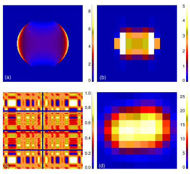
Figure 3: (a) The expected image at 28 $\mathrm{keV}$ (in units of 10^-26 ergs cm^-2 s^-1 Hz^-1 sr^-1) based on simulations performed by Reynolds (1999). (b) The sampled sky image in the ISGRI sky pixels size (in units of ct s^-1) . (c) The corresponding shadowgram of the PIF values and (d) the reconstructed image after the standard deconvolution (in units of ct s^-1).

The results of the analysis of the JEM-X and IBIS/ISGRI data of SN 1006 are presented in Kalemci et al. (2006). The source was not detected with ISGRI. Using the same method as in section 3.1, it was possible to extract an upper limit on the hard X-ray emission of SN 1006. Since the expected morphology is almost symmetric and the emission is concentrated in two extended limbs, the ratio between the maximal value in the reconstructed image at the position of each limb and their respective global flux provides a correction factor. In Kalemci et al. (2006), the ”standard” upper limits (obtained as if the SN 1006 is an unresolved source) were divided by this correction factor of $\sim$ 0.7 to take the flux dilution into account. Note that a relative reconstructed peak flux of 0.7 is close to what we obtained for an extended source of $\sim 10^{\prime}$ radius (see Fig. 2).

4 General method

We have shown that any coded mask imager such as IBIS works with extended sources just as predicted based on its SPSF properties: the reconstructed peak flux follows the simple flux dilution over the large number of unresolved points constituting an extended source. Moreover, as previously presented by Gros et al. (2003), the width of the IBIS SPSF varies within the FOV.

4.1 Reconstructed flux of extended sources

As described in section 3, the flux of a point-like source in a reconstructed IBIS image is given by the peak of the SPSF. Therefore, as shown in the previous sections, this will give a biased estimation of the flux of an extended source. For proper flux estimation, one needs to convert the reconstructed standard images into images of intensity (i.e. flux per solid angle or sky pixel), as is typical in astronomy. In that case, the global flux of any source (point-like or extended) would be given by integrating intensities over the source extent. The method is to divide standard flux images by the SPSF effective area (the solide angle subtended by the SPSF on the celestial sphere, i.e. the ratio between its integral and the peak value) but the main difficulty is that the shape of the IBIS SPSF varies within the FOV, so it is necessary to construct a map of its effective area (hereafter, $\tilde{A}$).

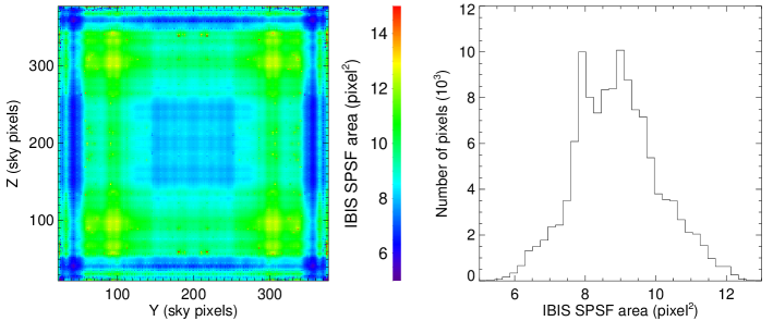
Figure 4: Map of the IBIS SPSF effective area $\tilde{A}$ in a linear scale (left) and the histogram of its values (right).

We have calculated point-like sources each $\sim 15^{\prime}$ (3 ISGRI sky pixels sampling) in the first quarter of the IBIS FOV with a fixed flux and fitted each corresponding reconstructed image at the source position by a 2D gaussian. We assume that these images must have a central symmetry due to that of the MURA coded mask and then we have projected each quarter of images where we performed the simulations on the three others according to the central symmetry. Figure 4 presents the map of $\tilde{A}$ of the IBIS SPSF and the histogram of its values. The map is almost flat in the FCFOV and the values globally increase in the PCFOV. Its histogram shows an appreciable dispersion ($\sigma$ $\sim$ 1.3 sky pixel²) with a mean value of 8.9 sky pixel². To obtain reconstructed sky images in intensity, one can then apply the following transformation:

$$I^{\prime}_{mn}=\frac{S^{\prime}_{OSA}}{\tilde{A}_{mn}}$$ (4)

$$I^{\prime}_{S}=\sum_{\Omega}I^{\prime}_{mn}$$ (5)

where S’_OSA is the reconstructed flux image obtained with the standard deconvolution. The legitimacy of such a transformation is shown in Appendix A.1 and is based on the sole assumption that $\tilde{A}$ does not change on scales smaller than the SPSF width. Thus, for extended sources simulated as described in section 2, we have built these intensity images $I^{\prime}_{mn}$. For each of them we have integrated over the source extent as seen by IBIS ($\Omega$, i.e. the physical size of the source convolved with the IBIS SPSF $\sim$ source radius plus 3 $\times\sigma_{spsf}$) and we have checked that this final value corresponds to the input global flux of our simulations with a dispersion of less than 10 %.

4.2 Tests on the Crab Nebula observations

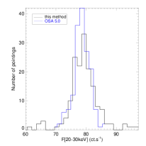
Figure 5: Left: Relative positions of the Crab Nebula for the 164 analyzed pointings during the rev. 102, 170. Right: Histograms of the reconstructed fluxes of the Crab with the standard analysis OSA 5.0 (in blue) and with our method (in black)

We have also tested this method on Crab Nebula observations. This source is considered as point-like for IBIS. We used data obtained during the revolutions 102, 170 and 300 containing 164 science windows (individual pointings, hereafter scws) and applied the same procedure as described above. Figure 5 presents the relative positions of the Crab for the analyzed scws and the histograms of the fluxes found with our method and the standard one in the 20-30 $\mathrm{keV}$ energy range. Even if our method shows a larger dispersion in the reconstructed Crab fluxes ($\sigma_{method}$ $\sim$ 3.1 s^-1 and $\sigma_{OSA5.0}$ $\sim$ 2.3 s^-1), the mean values are compatible (¡F_method¿ $\sim$ 78.9 s^-1 and ¡F_OSA5.0¿ $\sim$ 78.7 s^-1). Since the Crab Nebula is an unresolved source for IBIS, the reconstructed flux with our method depends on the source location since $\tilde{A}$ varies with the position in the field of view. However, the sensitivity of this dependence decreases with the source extent.

4.3 Estimation of the associated errors

Although the flux of any extended source can be measured with the method described above, the estimation of the corresponding errors is not simple. In fact, the reconstructed counts in the sky pixels within the SPSF of the IBIS telescope are correlated. Since we propose to sum the fluxes previously divided by $\tilde{A}$ over the size of the source, the associated variance should be $\sum{\sigma^{\prime 2}_{mn}/\tilde{A}^{2}_{mn}}$ ($\sigma^{\prime 2}_{mn}$ is the OSA flux variance) plus a covariance term. The latter depends on the position in the FOV and the source extent.

We have developed the standard equations of the convolution in Appendix A.2 to find a simple analytical expression of the variance associated to the equations 4 and 5 such that:

$$\sigma^{\prime 2}_{I^{\prime}_{S}}\approx\sigma^{2}_{B,ct.s^{-1}}\sum_{\Omega}\frac{1}{\tilde{E}_{mn}\tilde{A}_{mn}}$$ (6)

$$\sigma^{\prime 2}_{I^{\prime}_{S}}\approx\sum_{\Omega}\frac{\sigma^{\prime 2}_{OSA}}{\tilde{A}_{mn}}\approx N_{spsf}<\sigma^{\prime 2}_{OSA}>$$ (7)

where $\sigma^{2}_{B,ct.s^{-1}}$ is the detector variance of the background count rate (in units of count s^-2), ${E}_{mn}$ is the imaging efficiency and $<\sigma^{\prime 2}_{OSA}>$ is the OSA flux variance averaged over the region of pixel fluxes summation $\Omega$. N_spsf refers to the number of SPSFs within $\Omega$. Equation 7 can be interpreted as follows: the width of the SPSF ($\sigma_{spsf}$) is the correlation length of the instrument beyond which sky pixels are uncorrelated. Therefore, at these scales, the final variance associated with the reconstructed flux of an extended source by summing the pixel fluxes is simply given by the sum of the variances. This can be then approximated to the mean variance times the number of SPSFs within $\Omega$ (see Appendix B).

In order to check this analytical estimation of the associated error, we have performed Monte-Carlo simulations of extended sources seen through the IBIS coded mask as a sum of unresolved points. Shadowgrams are given by equation 2 for which we have added a constant background term. The total flux of each extended source was fixed at 50 s^-1 and that of the background at 10³ s^-1. 500 shadowgrams are simulated for different source sizes (assumed to be uniform disks), from 0^∘ (point-like) to 1^∘ radius, following the equation: $\sqrt{D_{kl}}\times{N(0,1)}+D_{kl}$ where D defines the ISGRI expected count rate shadowgram at the pixel (k,l). N(0,1) is the normal distribution. Each of these simulated shadowgrams was deconvolved using the standard method of the IBIS data analysis in order to obtain 500 reconstructed images in flux, variance and significance. We performed these calculations for three different source positions in the FOV: one on-axis (Y=200.5, Z=200.5) and two in the PCFOV at $\sim$ 9.5^∘ (Y=300.5, Z=250.5, labelled “Off Axis1”) and $\sim$ 13.5^∘ near the edge of the FOV (Y=120.5, Z=50.5, labelled “Off Axis2”). These calculations allow us to control the statistics for any source extent and position in the FOV. We have reconstructed the source fluxes using the method described in section 4.1 and measured the width of each flux histogram, which corresponds to the error associated to this method.

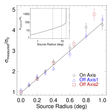
Figure 6: The ratio between the measured error of our method and that predicted for a point-like source ($\sigma_{0}$) as a function of the source radius for the three relative source positions. The solid line is given by the equation 6 and its large-scale behavior up to the total IBIS FOV is shown in the encapsulated plot.

Figure 6 presents the ratio between the measured error and that derived from the equation 6 for a point-like source (labelled $\sigma_{0}$) as a function of the source radius for the three distinct source positions. This ratio characterizes the loss in sensitivity due to the source extent. The error bars were calculated from the error of the fit performed on each reconstructed fluxes histogram to estimate the error of the method. For any source size and position, the dispersion is estimated to be less than 10 %.

5 Discussion

We have shown that it is always possible to obtain an estimate of the flux of any extended source with coded mask imaging. This is an intrinsic property of these imaging systems where the source flux is obtained through a linear combination of detector-pixel count rates. We have derived analytical expressions for estimating the global flux and its associated error of any extended sky source which were tested by Monte-Carlo simulations. This work was done relating to what one could expect to observe in the $\gamma$-ray domain through a MURA coded mask instrument such as IBIS onboard the INTEGRAL satellite. For IBIS, extended sources with a radius greater than $\sim$ 4.5^∘ will be confused with their associated ghosts. One will need a specific method to clean the images but this is beyond the scope of this paper. The advantage of this method, as long as the integration region contains all the source, is that the observer does not have to assume any source geometry during the analysis as is the case for methods using model fitting. Of course, in principle, the optimum signal to noise ratio is attained with the smallest integration region still containing all the source. However, due to the flux dilution, the geometry of the extended source is generally not apparent in the maps and the observer may not always be provided with a precise source geometry. Nevertheless, the signal to noise ratio does not decrease rapidly with the integration region size once the source is fully contained in it. In order to check the global method on an astrophysical case, we analyzed the IBIS/ISGRI data on the Coma Cluster, a bright known cluster of galaxies with an X-ray size of order $30^{\prime}$ diameter. We applied this method, increasing the integration region until a maximum signal to noise ratio was reached. In that way, we were able to extract for the first time the global intensity of this extended source as well as interesting constraints on its morphology. The results are presented in a joint paper Renaud et al. (2006). In a forthcoming paper, this method will be also used on the IBIS/ISGRI observations on the Vela Junior SNR (Renaud et al. 2006, in preparation).

Usually, the observer needs a lot of integration time for detecting an extended source ($\sim$ 5 $\times$ 10⁵ secondes for the Coma Cluster) and will have to construct mosaics of individual images. After obtaining the individual images with the standard analysis, the next step is to build mosaics as usual by weighting each image by their associated variance and transform them following the practical tips on the use of the method given in Appendix B. Any observer interested in this method may contact the first author to obtain the map $\tilde{A}$.

Appendix A Deconvolution Algorithm

In this section, we will adopt the following notations:

$$(k,l) \xrightarrow[]{} {\rm detector}$$ (8)

$$(i,j) \xrightarrow[]{} {\rm real}\hskip 2.84526pt{\rm sky}$$ (9)

$$(m,n) \xrightarrow[]{} {\rm reconstructed}\hskip 2.84526pt{\rm sky}$$ (10)

D is the detector, S and S’ the real and reconstructed skies, M the coded mask, R the decoding matrix, and B the background. By definition:

$$D_{kl} = \sum_{ij}S_{i,j}M_{i+k,j+l}+B_{k,l}$$ (11)

$$S^{\prime}_{mn} = \sum_{kl}R_{k+m,l+n}D_{kl}$$ (12)

with the following arrays:

$$R_{k+m,l+n} = \frac{G^{+}_{k+m,l+n}-Bal_{mn}\times{G^{-}_{k+m,l+n}}}{E_{mn}}$$ (13)

$$Bal_{mn} = \frac{\sum_{kl}G^{+}_{k+m,l+n}}{\sum_{kl}G^{-}_{k+m,l+n}}$$ (14)

$$E_{mn} = \sum_{kl}G^{+}_{k+m,l+n}M_{k+m,l+n}-Bal_{mn}\sum_{kl}G^{-}_{k+m,l+n}M_{k+m,l+n}$$ (15)

where G⁺, G^- the decoding arrays related to the coded mask M (see Goldwurm et al. 2003), Bal_m,n is called the balance array in order to have a flat reconstructed flux image and E_m,n correponds to the imaging efficiency to correct for partial exposure outside the FCFOV.

A.1 Reconstructed fluxes

The standard reconstructed flux image is given by:

$$S^{\prime}_{mn}=\sum_{kl}R_{k+m,l+n}\sum_{ij}S_{ij}M_{i+k,j+l}+\sum_{kl}R_{k+m,l+n}B_{k,l}$$ (16)

We propose to construct images of flux per steradian (per sky pixel) I’${}_{mn}=S^{\prime}_{mn}/\tilde{A}_{mn}$ where $\tilde{A}_{mn}$ is the SPSF area. The global flux of any source (point-like or extended) I’_S is then given by the sum of the intensities within a region $\Omega$ encompassing the source extent. Therefore:

$$I^{\prime}_{S}=\sum_{\Omega}\frac{1}{\tilde{A}_{mn}}\sum_{ij}S_{ij}\sum_{kl}R_{k+m,l+n}M_{i+k,j+l}+\sum_{\Omega}\frac{1}{\tilde{A}_{mn}}\sum_{kl}R_{k+m,l+n}B_{k,l}$$ (17)

Assuming that the detector D was well background-substracted before the deconvolution, the second term of the right-hand side of the above equation is null.

$\tilde{A}_{mn}$ represents the integrated normalized SPSF. By definition, we have:

$$SPSF_{ij}(m,n) = \sum_{kl}R_{k+m,l+n}M_{i+k,j+l}$$ (18)

$$\tilde{A}_{mn} = \sum_{m^{\prime},n^{\prime}\in K^{m,n}}SPSF_{mn}(m^{\prime},n^{\prime})$$ (19)

where SPSF_ij(m,n) is the SPSF value at the position (m,n) of the source at the position (i,j) with a unit-flux. K^m,n defines the local region encompassing the SPSF of the point source at the position (m,n). Substituting equation 18 in 17:

$$I^{\prime}_{S} = \sum_{ij}S_{ij}\sum_{m,n\in\Omega}\frac{SPSF_{ij}(m,n)}{\tilde{A}_{mn}}$$ (20)

$$= \sum_{ij}S_{ij}\sum_{m,n\in K^{i,j}}\frac{SPSF_{ij}(m,n)}{\tilde{A}_{mn}}$$ (21)

For each point source S_ij, we have reduced the sum over $\Omega$ (i.e. the source extent) to the sum over K^i,j, the local region around the point source at (i,j). Thus, if we assume for each unresolved point that $\tilde{A}_{mn}=\tilde{A}_{ij}$ is constant within K^i,j, we finally obtain:

$$I^{\prime}_{S}\approx\sum_{ij}S_{ij}$$ (22)

A.2 Reconstructed variances

From equation 16, the reconstructed flux variance is given by:

$$\sigma^{\prime 2}_{S^{\prime},mn}=\sum_{ij}\sigma^{2}_{S,ij}(\sum_{kl}R_{k+m,l+n}M_{i+k,j+l})^{2}+\sum_{kl}\sigma^{2}_{B,kl}R_{k+m,l+n}^{2}$$ (23)

where $\sigma^{2}_{S,ij}$ is the variance related to the celestial source at the position (i,j) and $\sigma^{2}_{B,kl}$ that related to the detector background. $\sigma^{\prime 2}_{S^{\prime},mn}$ is equivalent to the OSA flux variance $\sigma^{\prime 2}_{OSA}$.

In most cases in the high-energy domain, the variance due to the celestial source(s) is very small compared to that due to the background count rate. Therefore, in the calcul of the variance associated to the transformation I’${}_{S}=\sum_{\Omega}S^{\prime}_{mn}/\tilde{A}_{mn}$, the contribution of the first term in equation 17 can be neglected. Given that the detector pixels are independent, we obtain:

$$\sigma^{\prime 2}_{I^{\prime}_{S}}=\sigma^{2}_{B}\sum_{kl}\left(\sum_{\Omega}\frac{R_{k+m,l+n}}{\tilde{A}_{mn}}\right)^{2}$$ (24)

In the above equation, we have assumed for simplicity that the detector variance $\sigma^{2}_{B,kl}$ is spatially constant. As the decoding arrays G⁺ and G^- are given by (2M - 1)⁺ and (2M - 1)^-, respectively, we obtain:

$$\sigma^{\prime 2}_{I^{\prime}_{S}} \approx 2\sigma^{2}_{B}\sum_{kl}\sum_{\Omega_{1},\Omega_{2}}\frac{R_{k+m1,l+n1}(M^{+}_{k+m2,l+n2}-Bal_{m2,n2}M^{-}_{k+m2,l+n2})}{\tilde{A}_{m1,n1}\tilde{A}_{m2,n2}E_{m2,n2}}$$

$$- \sigma^{2}_{B}\sum_{kl}\sum_{\Omega_{1},\Omega_{2}}\frac{R_{k+m1,l+n1}(1^{+}-Bal_{m2,n2}\times{1^{-}})}{\tilde{A}_{m1,n1}\tilde{A}_{m2,n2}E_{m2,n2}}$$ (25)

In the FCFOV, the balance array is almost -1 and only varies within $\sim$ 5 % in the PCFOV. Therefore:

$$\sigma^{\prime 2}_{I^{\prime}_{S}} \approx 2\sigma^{2}_{B}\sum_{kl}\sum_{\Omega_{1},\Omega_{2}}\frac{R_{k+m1,l+n1}.M_{k+m2,l+n2}}{\tilde{A}_{m1,n1}\tilde{A}_{m2,n2}E_{m2,n2}}$$ (26)

$$- \sigma^{2}_{B}\sum_{kl}\sum_{\Omega_{1},\Omega_{2}}\frac{R_{k+m1,l+n1}.1}{\tilde{A}_{m1,n1}\tilde{A}_{m2,n2}E_{m2,n2}}$$ (27)

The second term of the equation is assumed to be 0, since the deconvolution of any flat image gives a reconstructed sky of 0 values. We have expanded the first term, following the above definitions of $\tilde{A}$ and R, and finally found a simple expression for the associated intensity variance such that:

$$\sigma^{\prime 2}_{I^{\prime}_{S}} \approx \sigma^{2}_{B,ct.s^{-1}}\sum_{\Omega}\frac{1}{\tilde{E}_{mn}\tilde{A}_{mn}}$$ (28)

$$\sigma^{2}_{B,ct.s^{-1}} = \frac{\sum_{kl}D_{k,l}}{{\rm Time}^{2}}$$ (29)

$$\tilde{E}_{mn} = \frac{E_{mn}}{{\rm On-Axis\hskip 0.56905ptAperture}}$$ (30)

In this expression, the final variance $\sigma^{\prime 2}_{I^{\prime}_{S}}$ is in count s^-2 for homogeneity with I’_S (in count s^-1). The On-Axis Aperture is the number of detector pixels which are illuminated through the mask by an on-axis source ($\approx$ half of the ISGRI camera, i.e. 8192 pixels) and $\tilde{E}_{mn}$ is the imaging efficiency of the telescope.

Appendix B Practical tips on the use of the method

Equation 28 presents a simple expression of the intensity variance associated with the method we developed for reconstructing the flux of an extended source. In order to provide the observer analyzing the IBIS data with an easy-to-use expression, in relation to the standard OSA sky maps, we found that:

$$\sigma^{\prime 2}_{OSA}\approx\frac{\sigma^{2}_{B,ct.s^{-1}}}{\tilde{E}_{mn}}$$ (31)

and then, from equation 28:

$$\sigma^{\prime 2}_{I^{\prime}_{S}}=\sum_{\Omega}\frac{\sigma^{\prime 2}_{OSA}}{\tilde{A}_{mn}}$$ (32)

If $\tilde{A}$ does not suffer from large variations over $\Omega$, one may approximate the last equation:

$$\sigma^{\prime 2}_{I^{\prime}_{S}}\approx<\sigma^{\prime 2}_{OSA}>\times{\frac{N_{pix}}{<\tilde{A}>}}=N_{spsf}<\sigma^{\prime 2}_{OSA}>$$ (33)

where $\sigma^{\prime 2}_{OSA}$ is an estimate of the OSA flux variance averaged over $\Omega$. The sum in equation 32 is reduced to the number of sky pixels within $\Omega$ divided by $<\tilde{A}>$, i.e. the number of IBIS SPSFs. The transformation $S^{\prime}_{OSA}\rightarrowtail{I^{\prime}}$ allows the construction of sky images where anybody may integrate intensities over any region $\Omega$ in order to properly measure the global flux of an extended source. The associated variance is then given by equation 32. The following equations allow the user to construct mosaics of a set of individual images:

$$S^{\prime}_{mosaic} = \frac{\sum{S^{\prime}_{OSA}/\sigma^{\prime 2}_{OSA}}}{\sum{1/\sigma^{\prime 2}_{OSA}}}$$ (34)

$$\tilde{A}_{mosaic} = \frac{\sum{\tilde{A}/\sigma^{\prime 2}_{OSA}}}{\sum{1/\sigma^{\prime 2}_{OSA}}}$$ (35)

$$\sigma^{\prime 2}_{mosaic} = \frac{1}{\sum{1/\sigma^{\prime 2}_{OSA}}}$$ (36)

As for an individual image, the global flux and the associated error of an extended source will be given by:

$$I^{\prime}_{S} = \sum_{\Omega}\frac{S^{\prime}_{mosaic}}{\tilde{A}_{mosaic}}$$ (37)

$$\sigma^{\prime 2}_{I^{\prime}_{S}} = \sum_{\Omega}\frac{\sigma^{\prime 2}_{mosaic}}{\tilde{A}_{mosaic}}$$ (38)