Time Dependent Monte Carlo Radiative Transfer Calculations For 3-Dimensional Supernova Spectra, Lightcurves, and Polarization

Abstract

We discuss Monte-Carlo techniques for addressing the 3-dimensional time-dependent radiative transfer problem in rapidly expanding supernova atmospheres. The transfer code SEDONA has been developed to calculate the lightcurves, spectra, and polarization of aspherical supernova models. From the onset of free-expansion in the supernova ejecta, SEDONA solves the radiative transfer problem self-consistently, including a detailed treatment of gamma-ray transfer from radioactive decay and with a radiative equilibrium solution of the temperature structure. Line fluorescence processes can also be treated directly. No free parameters need be adjusted in the radiative transfer calculation, providing a direct link between multi-dimensional hydrodynamical explosion models and observations. We describe the computational techniques applied in SEDONA, and verify the code by comparison to existing calculations. We find that convergence of the Monte Carlo method is rapid and stable even for complicated multi-dimensional configurations. We also investigate the accuracy of a few commonly applied approximations in supernova transfer, namely the stationarity approximation and the two-level atom expansion opacity formalism.

1. Introduction

1.1. Motivations

Most of what we know about supernovae (SNe) has been learned from observations of the lightcurve, spectrum, and polarization of the supernova light during the months and years following the explosion. Except for most nearby events, the explosion process itself is never directly observed, and the progenitor star system only rarely. What we do see is emission from the hot, radioactive material ejected in the explosion. Theoretical radiative transfer modeling of the emission is needed to discern the physical conditions in the SN ejecta, offering insight into the physics of the explosion itself and the progenitor star system which gave rise to it.

One dimensional (1D) explosion models of SNe have been used to synthesize emergent spectra and light curves in reasonable agreement with observed ones. Because nearly all observed SNe are too distant to be resolved in the early phases, deviations from spherical symmetry can not be directly imaged. Nevertheless, three lines of observational evidence imply that the ejecta possess an interesting multi-dimensional structure: (1) The detection of a non-zero intrinsic polarization in SNe of all types, indicating a preferred direction in the scattering medium (e.g., Cropper et al., 1988; Kawabata et al., 2002; Wang et al., 2003; Leonard et al., 2005); (2) The appearance of unusual flux features in some SNe, naturally explained by a clumpy ejecta structure, e.g., the “Bochum event” in SN 1987A, (Hanuschik & Dachs, 1987; Utrobin et al., 1995); (3) The complex morphologies of SN remnants, which show clumpy, filamentary, or jet-like structures (Fesen & Gunderson, 1996; Hwang et al., 2000; Decourchelle et al., 2001).

Most current theoretical SNe explosion scenarios involve multi-dimensional effects in an essential way. In hydrodynamical explosion models, ejecta asymmetries arise, for example, from random instabilities in the explosion physics, e.g., Rayleigh Taylor instabilities, convective mixing (Chevalier & Klein, 1978; Burrows et al., 1995; Kifonidis et al., 2000; Gamezo et al., 2003; Röpke & Hillebrandt, 2005); from anisotropic energy ejection mechanisms, e.g., jets, off-center ignition (Khokhlov et al., 1999; MacFadyen & Woosley, 1999; Plewa et al., 2004), or from asphericities in the progenitor star or its surrounding medium, e.g., rapid rotation of the progenitor, the presence of a binary companion star (Marietta et al., 2000; Yoon & Langer, 2005).

The multi-D explosion models make predictions as to the velocity, composition and geometry of the material ejected in the SN explosion. To confront such predictions with observations, the multi-D radiative transfer problem in expanding SN atmospheres must be addressed. Detailed radiative transfer codes synthesize model spectra, light curves and polarization which can be compared directly to observations. Such transfer codes can also be usefully applied in an empirical “inverse” approach, in which hand-tailored, parameterized ejecta configurations are used to extract model-independent information directly from the observations.

Here we describe a Monte Carlo approach to the multi-dimensional time-dependent radiative transfer problem in expanding SN atmospheres, embodied in the transfer code SEDONA. Given an arbitrary 3-dimensional ejecta structure (i.e., the density, composition and velocity structure of freely expanding SN material) SEDONA self-consistently calculates the emergent broadband light curves, spectral time-series (in both optical and gamma-rays) and polarization spectra from various viewing angles. No free parameters need be adjusted in the transfer calculations, providing a direct link between multi-dimensional hydrodynamical explosion models and observations. In this paper, we describe the radiative transfer techniques used in SEDONA, and give some examples of its verification and application.

1.2. Monte Carlo Radiative Transfer

In the Monte-Carlo (MC) approach to radiative transfer, packets of radiant energy (“photons”) are emitted from within the SN envelope and tracked through random scatterings and absorptions until they escape the atmosphere. Each photon packet possesses a specific wavelength and polarization state which are updated at each interaction event. Tallies of photon packets can be used to construct estimators of the local radiation field properties and the emergent spectrum at infinity. The calculated quantities possess statistical noise, which is reduced as the number of propagated packets is increased.

The MC approach has several advantages over direct numerical solution of the radiative transfer equation. MC codes are intuitive, relatively easy to develop, and generally less likely to fall victim to subtle numerical errors (Auer, 2003). The method generalizes readily to multi-dimensional time-dependent problems and the inclusion of polarization. As discussed in detail below (§3.4), convergence of MC calculations is found to be stable and rapid even for complicated configurations. Finally, although MC techniques can be computational expensive, they parallelize well and can be profitably run on multi-processor supercomputers.

Monte Carlo approaches have been applied to a wide range of astrophysical radiative transfer problems, including multi-dimensional polarization problems (e.g., Daniel, 1980; Code & Whitney, 1995; Wood et al., 1996). The MC code described in Höflich et al. (1996) has been used to calculate the continuum polarization and polarization spectrum of 2-D SN (Höflich, 1991; Wang et al., 1997; Howell et al., 2001). In addition, the 1-D MC code of Mazzali & Lucy (1993) has been used in numerous studies of SN flux spectra (e.g., Mazzali et al., 1995, 2001). The papers of Leon Lucy have been particularly important in developing the MC technique for astrophysical applications (Lucy, 1999a, b, 2001, 2002, 2003, 2005a, 2005b). The new techniques, many of which are applied here, make it feasible for MC codes to match the physical accuracy of formal solutions of the radiative transfer equation.

2. Structure of the Radiative Transfer Code

2.1. Overview of Technique

A short time after the eruption of a SN, hydrodynamic and nucleosynthetic processes abate and the ejected material reaches a phase of near free expansion. Thereafter, the essential theoretical challenge becomes to simulate the diffusion of photons through the hot and optically thick ejecta – i.e., the radiative transfer problem. For epochs around and prior to peak brightness, the diffusion time of photons exceeds the expansion time, such that the fully time-dependent radiative transfer equation must be addressed. In this case, MC photon packets must be propagated through both space and time.

The SEDONA code takes as input the density, composition, and shock deposited energy specified at initial time $t_{0}$ at every point on a spatial grid. The spatial grid can be defined in a variety of coordinate systems, including 1-D spherical, 2-D cylindrical, and 3-D Cartesian systems. In the free-expansion phase, the velocity of the ejecta is homologous and everywhere proportional to radius: $r=vt_{\mathrm{exp}}$ where $t_{\mathrm{exp}}$ is the time since explosion. Given the self-similar nature of the flow, velocity is used as the spatial coordinates in the simulation, i.e., the spatial grid expands along with the flow.

A separate spatial grid exists for each time step in the model. The time discretization in the model most be chosen fine enough to resolve the expansion of the SN ejecta. Typically of order 100 logarithmically spaced time steps are used. Following homology, the density in a cell decreases with time as $(t/t_{0})^{-3}$ while the composition remains fixed. The evolution of the local radiation field and temperature in the cell are determined by the Monte Carlo propagation of photon packets, as described below.

Propagation of the MC photon packets requires knowledge of the opacity and emissivity of the SN ejecta at all points on the space-time grid. In general, these quantities depend upon the local radiation field which heats and excites the gas. Because the state of the radiation field can only be known after the MC simulation has been run, an iterative approach is necessary to arrive at a self-consistent model. The overall iterative structure of the transfer code is described as follows:

1. Using a 3-D gamma-ray transfer routine, we determine the rate of energy deposition in each cell from the decay of radioactive ${}^{56}\mathrm{Ni}$ and ${}^{56}\mathrm{Co}$. This, along with any initial shock deposited energy, serves as the source geometry for the optical photon packets.

2. The opacities and emissivities at all wavelengths for each cell and at each time step are computed. Because the cell temperatures at each time are not initially known, we start with a reasonable guess, to be refined iteratively.

3. The propagation of optical photon packets through space and time is followed, providing suitable tallies of the photon absorption rate in each cell.

4. A new temperature is determined for each point on the space-time grid by setting the rate of thermal emission equal to the calculated rates of photon absorption plus any radioactive energy deposition.

5. The temperature structures calculated in step (4) will differ from that used to compute the opacities in step (2). Thus, to bring about consistency, we recompute the opacities/emissivities and return to step (3), iterating this procedure until the temperature and opacities change negligibly from one iteration to the next.

6. Once the model atmosphere has converged, the synthetic lightcurves and flux and polarization spectra are generated during step (3) by collecting all photon packets escaping the atmosphere along a certain line of sight.

Before discussing each step in detail, we mention the important physical approximations made in the present version of the code.

1. Homologous Expansion: We assume the SN ejecta is in free expansion, with a homologous velocity structure. Thus the velocity field of the ejecta is always spherically symmetric, even if the ejecta density structure is not. Free expansion is approached when the ejecta have expanded sufficiently that the kinetic energy density well exceeds the gravitational and internal energy densities. In Type Ia SN, this occurs less than a minute after the explosion (Röpke, 2005); for Type II SN, it can take as long as several days (Herant & Woosley, 1994). At later times, the energy input from the decay of newly synthesized radioactive isotopes may produce non-negligible deviations from homology (Pinto & Eastman, 2000b). Note that SEDONA does take into account adiabatic losses of the radiation field, but in keeping with homology assumes that the ejecta structure is negligibly affected by the energy exchange. The current calculations also neglect relativistic corrections going as $(v/c)^{2}$, although these can be easily included if needed (Lucy, 2005b).

2. The Sobolev Approximation: For atmospheres with large velocity gradients such as SNe, the Sobolev approximation provides a simple and elegant treatment of line transfer (Sobolev, 1947). Detailed derivations of the Sobolev formalism are given in (Mihalas, 1978; Jeffery & Branch, 1990; Castor, 1970). The underlying physical assumption is that the intrinsic profile of bound-bound transitions is vanishingly narrow. This is an excellent approximation in SN atmospheres, in which the Doppler velocity width of lines ($v_{d}\approx 5~{}\mathrm{km~{}s}^{-1}$) is typically much less than the velocity scale over which the ejecta properties change ($v\approx 1000~{}\mathrm{km~{}s}^{-1}$). Formal inaccuracy may occur if the ejecta contain numerous small scale structures or for very optically thick lines in which the Lorentz wings become important. In addition, Baron et al. (1996) have emphasized the problem that, given the enormous number of iron-peak lines at ultraviolet wavelengths, several hundreds of lines may overlap within a single Doppler width. This overlapping clearly violates the assumptions under which the Sobolev formalism is derived, although it difficult to assess what sort of practical implications this has on the transfer calculations. The vast majority of the overlapping lines are exceedingly weak, and the velocity spacing of optically thick lines (which dominate the spectrum formation) is typically much larger than a Doppler width (Jeffery, 1995). The errors thus incurred on the emergent spectra are thus too small to notice, at least in the few test calculations performed so far (Eastman & Pinto, 1993). However, further head-to-head comparisons (including non-equilibrium effects) are clearly needed. For now, given the memory constraints of current computing facilities, the Sobolev approximation appears unavoidable in multi-D time-dependent calculations, for which the opacity of an enormous number of lines must be stored on an extensive space-time grid. In this context, one anticipates any error incurred to cause quantitative, not qualitative, variations in the emergent spectra and lightcurves, and will likely not obscure the basic model dependencies and orientation effects we are interested in studying.

3. Equilibrium Assumptions: In the present models, we assume the ionization/excitation state of the SN gas follows local thermodynamic equilibrium (LTE) and can be calculated using the Saha ionization and Boltzmann excitation equations. We do not, however, require the radiation field to be in equilibrium, and can include scattering and fluorescence processes in the line source functions. While the microscopic conditions for LTE (i.e., the dominance of collisional rates) are not met in the rarefied atmospheres of SNe, deviations of the atomic level populations from LTE should generally cause quantitative, not qualitative differences in the emergent spectra. For Type Ia SN, non-LTE effects are found to be small near maximum light (Baron et al., 1996), but become increasingly important several months after the explosion. A solution to the non-LTE rate equations in the context of the Sobolev approximation is readily incorporated into the MC approach (see Li & McCray, 1993; Zhang & Wang, 1996; Lucy, 2003) and future versions of SEDONA will include such a solution for selected ionic species.

2.2. Calculation of Opacities and Emissivities

The important opacities in SN atmospheres are electron scattering, bound-bound line transitions and, to a much lesser extent, bound-free and free-free opacities. With the temperature, density and composition of the ejecta given, the LTE ionization and excitation of the gas are determined by solving the Saha ionization and Boltzmann excitation equations coupled to the equation of charge conservation.

Standard formulae for the extinction coefficients for electron scattering and free-free opacities are found in e.g., Rybicki & Lightman (1986). We take bound-free opacities from the Opacity Project (Cunto & Mendoza, 1992) when available, otherwise the hydrogenic approximation is applied. All continuum opacities are stored in discrete wavelength bins.

For the case of a single bound-bound transition, the extinction coefficient is given by

$$\alpha_{bb}=K_{lu}\phi(\lambda),$$ (1)

where $\phi$ is the line profile in the wavelength representation and $K_{lu}$ is the (dimensionless) integrated line strength given by

$$K_{lu}=\biggl{(}\frac{\pi e^{2}}{m_{e}c}\biggr{)}fN_{l}(\lambda_{0}^{2}/c)\biggl{(}1-\frac{N_{u}g_{l}}{N_{l}g_{u}}\biggr{)},$$ (2)

where $f$ is the oscillator strength of the transition, $\lambda_{0}$ the line center rest wavelength, and $N_{l}$ and $N_{u}$ are the number density of the lower and upper atomic levels respectively. The last term in parentheses is the correction for stimulated emission, where $g_{l}$ and $g_{u}$ are the statistical weights of the lower and upper atomic levels.

In a differentially expanding atmosphere, propagating photons are continually Doppler shifting with respect to the local comoving frame. The opacity of a bound-bound transition is thus only experienced when a photon Doppler shifts into resonance with the line. In the Sobolev approximation, the spatial extent of the region of resonance is assumed negligible, and the optical depth across the resonance region is given by the Sobolev line optical depth

$$\tau=\frac{K_{\lambda}ct_{\mathrm{exp}}}{\lambda_{0}}.$$ (3)

This simple equation only holds for atmospheres in homologous expansion; for other velocity laws $\tau$ will depend upon the direction the photon packet is traveling.

The probability of a photon interacting with the line is $1-\exp(-\tau)$. In general, a photon will scatter multiple times in the resonance region before escaping the line, where the escape probability is given by

$$\beta=\frac{1-e^{-\tau}}{\tau}.$$ (4)

The conventional $\beta$ notation for the escape probability should not be confused with the relativistic speed parameter $\beta=v/c$.

The result of the interaction of a photon with a line is the redirection of the photon and its possible wavelength redistribution. We consider three relevant atomic processes: pure scattering, absorption/re-emission, and fluorescence. The probability of the photon being absorbed in the transition with lower level $l$ and upper level $u$ is given by (Pinto & Eastman, 2000b)

$$p_{\mathrm{abs}}=\frac{N_{e}\sum_{k}C_{uk}}{N_{e}\sum_{k}C_{uk}+\sum_{k}\beta_{uk}A_{uk}}$$ (5)

here $N_{e}$ is the electron density, $C_{uk}$ the collision coefficient, and $A_{uk}$ the Einstein spontaneous de-excitation coefficient. The sums runs over over all levels $k$ accessible from the upper level $u$. Collisonal coefficients can be calculated approximately using Van Regemorter’s formulae (van Regemorter, 1962).

For the conditions in SN atmospheres, the probability of true absorption is found to be very small $p_{\mathrm{abs}}\approx 10^{-6}-10^{-4}$. It is much more likely that the atom radiatively de-excites and, more often than not, the de-excitation is a fluorescence into an atomic level different than the original lower level (Pinto & Eastman, 2000b).

Atomic line data for the bound-bound transitions (including the oscillator strengths and energy level data) have been taken from CD 23 and CD 1 of Kurucz & Bell (1995), containing over 500,000 and 40 million lines respectively. Forbidden lines are not included in the present calculations. In practice, it is often impossible to store the optical depths for this many lines for all points on the space time-grid. Thus, for most calculation we select a subset (typically from 0 to 500,000) of the most important lines to be given an individual direct treatment with a more detailed approximation of fluorescence. All remaining lines are treated approximately by combining them into a discrete opacity grid using the expansion opacity formalism introduced by Karp et al. (1977) and later reformulated by Eastman & Pinto (1993)

$$\alpha_{\mathrm{exp}}(\lambda_{\mathrm{c}})=\frac{1}{ct_{\mathrm{exp}}}\sum_{i}\frac{\lambda_{i}}{\Delta\lambda_{\mathrm{c}}}(1-e^{-\tau_{i}}),$$ (6)

where $\lambda_{\mathrm{c}}$ is the central wavelength of the bin and the sum runs over all lines in the bin of width $\Delta\lambda_{c}$. Preferably, the wavelength bin sizes are $\lesssim 10~{}\AA$, to achieve reasonably well resolved spectra. The source function for these lines is treated in the two-level atom (TLA) formulation

$$S_{\lambda}=(1-\epsilon)\bar{J}_{\lambda}+\epsilon B_{\lambda}(T).$$ (7)

where $\epsilon$ represents the probability of absorption. In general, the value of $\epsilon$ is unique for each line and can be calibrated by comparison to NLTE results (Höflich, 1995). In the present case, we follow the approach of Nugent et al. (1997), and choose $\epsilon$ a common value for each line. The validity of this TLA approximation is investigated in §3.6.

One can also define a purely absorptive component of the line expansion opacity

$$\alpha_{\mathrm{abs,exp}}(\lambda)=\frac{1}{ct_{\mathrm{exp}}}\sum_{i}\frac{\lambda_{i}}{\Delta\lambda_{\mathrm{c}}}\biggl{[}\frac{\epsilon}{\beta+\epsilon(1-\beta)}\biggr{]}(1-e^{-\tau_{i}}),$$ (8)

as well as an purely absorptive component of the opacity from the lines treated directly

$$\alpha_{\mathrm{abs,line}}(\lambda)=\frac{1}{ct_{\mathrm{exp}}}\sum_{i}\frac{\lambda_{i}}{\Delta\lambda_{\mathrm{c}}}p_{\mathrm{abs}}(1-e^{-\tau_{i}}).$$ (9)

The total absorptive opacity from all sources is

$$\alpha_{\mathrm{abs}}=\alpha_{\mathrm{abs,line}}+\alpha_{\mathrm{abs,exp}}+\alpha_{\mathrm{bf}}+\alpha_{\mathrm{ff}},$$ (10)

while the thermal emissivity from all sources is

$$j_{\lambda}(\lambda)=B(\lambda)\alpha_{\mathrm{abs}}$$ (11)

2.3. Monte Carlo Transfer

The optical photon packets used in the MC simulation are monochromatic, equal energy packets. Each packet has initial energy $E_{p}$ and represents a collection of $N_{p}=E_{p}\lambda/hc$ photons of wavelength $\lambda$. The comoving frame energy of the packet is kept fixed throughout any absorption/scattering interaction, even if the packet wavelength is changed by the event. The benefit of this approach (as pointed out by Lucy (1999a)) is that energy is strictly conserved in each packet interaction. This allows for rapid convergence the correct temperature structure when the condition of radiative equilibrium is imposed (§3.4).

2.3.1 Emission of Photon Packets

The luminosity of a SN is powered by the decay of radioactive isotopes and/or thermal energy deposited by the SN shock-wave. The primary radioactive energy arises from the decay chain ${}^{56}\mathrm{Ni}$ $\rightarrow$ ${}^{56}\mathrm{Co}$ $\rightarrow$ ${}^{56}\mathrm{Fe}$, with nearly all of the decay energy emerging as $\sim 1$ MeV gamma-rays. At early times, these gamma-rays deposit energy in the ejecta primarily through Compton scattering and photo-electric absorption. Here we assume the deposited energy is thermalized locally and instantaneously, although non-thermal effects can readily be incorporated into the MC approach.

We determine the rate of radioactive energy deposition by following the emission and propagation of gamma-rays using a MC routine (see Milne et al., 2004, and references therein). Details of the routine are given in the Appendix. The gamma-ray transfer routine also supplies the gamma-ray lightcurve and time-series of emergent gamma-ray spectra as viewed from various inclinations. These are potentially powerful probes of the geometry and composition of the SN ejecta (Hungerford et al., 2003; Höflich, 2002).

The calculated energy deposition rate in each cell along with the inputted amount and distribution of internal shock deposited energy existent at the initial time $t_{0}$ serve as the source of photon packets. All photon packets in the simulation (regardless of emission time or location) are given the same initial energy $E_{p}$ in the comoving frame, where

$$E_{p}=\frac{1}{N_{p}}\biggl{[}E_{\mathrm{int,tot}}+E_{\mathrm{dep,tot}}\biggr{]},$$ (12)

where $E_{\mathrm{int,tot}}$ is the total amount of shock deposited and $E_{\mathrm{dep,tot}}$ the total time-integrated radioactively deposited energy. $N_{p}$ is the number of photon packets used in (each iteration of) the simulation. A fraction $E_{\mathrm{int,tot}}/E_{p}N_{p}$ of the photon packets arise from the shock deposited energy and so are emitted at the initial time $t_{0}$, and from a location sampled from the spatial distribution of shock energy. All remaining packets arise from the radioactive energy deposition, and are emitted at a time and location sampled from the instantaneous rate of energy deposition as determined by the gamma-ray transfer procedure. Emission is assumed isotropic in the comoving frame, with the packet wavelength sampled from the local thermal emissivity function (Eq. 11).

Given the above prescription for packet emission, there is no need to specify an inner boundary surface in the transfer simulation. Optical photon packets are allowed to traverse the entire ejecta, even the optically thick central regions. This represents an improvement over previous supernova MC codes (e.g., Mazzali & Lucy, 1993) in which photon packets are emitted from the surface of an extended spherical inner core, with any packet backscattered onto the core assumed to be “absorbed” and removed from the calculation.

2.3.2 Propagation of Photon Packets

Once emitted, photon packets are moved through the space-time grid in small steps in velocity space. The propagation of packets resembles that described in other MC studies (Mazzali & Lucy, 1993; Lucy, 2005a). A velocity step of size $v$ corresponds to a physical distance $vt_{\mathrm{exp}}$ and results in an elapse of time of $\delta t=t_{\mathrm{exp}}v/c$. In this way, packets are propagated through space and forward in time until they reach the outer edge of the spatial grid, and which point they are counted as being observed at the time of escape (§2.5).

Because of the differential expansion of the ejecta, the wavelength of a propagating photon is continually Doppler shifting with respect to the local comoving frame. In a homologously expanding atmosphere, this shift is always to the red and by an amount proportional to the distance traveled: $\Delta\lambda=\lambda v/c$. Photon packets come into resonance with spectral lines one by one (given our assumption of the Sobolev approximation) moving from blue to red. The velocity distance a packet propagates before coming into resonance with a line treated individually (i.e., not in the expansion opacity formalism) is

$$v_{l}=c(\lambda_{0}-\lambda)/\lambda_{0},$$ (13)

where $\lambda$ is the comoving frame wavelength of the packet and $\lambda_{0}$ is the rest wavelength of the line. Meanwhile the velocity distance a packet propagates before undergoing a continuum interaction with the matter is determined randomly by

$$v_{c}=-\frac{1}{\alpha t_{\mathrm{exp}}}\log(z),$$ (14)

where $\alpha$ is the total continuum opacity (i.e., the sum of the bound-free, free-free, electron-scattering and line expansion opacities) and $z$ is a random number uniformally sampled between 0 and 1, exclusive of the zero. The next event for the packet is determined by selecting the smallest value among $v_{l},v_{c},$ and $v_{s}$, where $v_{s}$ is the shorter of the distance to the cell boundary in the current direction of flight and the distance $c(t_{i}-t_{current})$ where $t_{i}$ is the next time boundary.

If a continuum interaction occurs, the possible fate of the packet is an absorption, electron scattering, or expansion-opacity line scattering. The nature of the event is determined by randomly sampling the local scattering and absorption fractions. An absorbed packet is assumed thermalized and immediately re-emitted with a new wavelength sampled from the local thermal emissivity (Eq. 11). For scattered packets, the comoving wavelength remains unchanged. Electron scattering differs from line expansion opacity scattering in its effect on the packet’s polarization state (see §2.3.3).

When a packet comes into resonance with a line being treated directly (i.e., not binned into the expansion opacity) an interaction occurs if

$$z<1-\exp(-\tau).$$ (15)

If an interaction does occur, the packet will either be absorbed (with probability given by Equation 5) or will radiatively de-excite. In the case of radiative de-excitation, the probability that the packet de-excites to atomic level $j$ is

$$p_{\mathrm{uj}}=\frac{\lambda_{j}^{-1}\beta_{uj}A_{uj}}{\sum_{k}\lambda_{k}^{-1}\beta_{uk}A_{uk}},$$ (16)

where the Einstein $A$ coefficients of each line have been weighted by the escape probabilities $\beta$ (in order not to count those emissions that do not escape the line resonance region and almost immediately re-excite the atom) and by the inverse wavelength of the lines in order to get the energy distribution of the fluorescence correct.

For every interaction event, a new propagation direction of the packet is chosen randomly from an isotropic distribution (except in the case of electron scattering, see §2.3.3). The new outgoing rest frame energy is

$$E_{\mathrm{out}}=E_{\mathrm{in}}\frac{1-\mu_{\mathrm{in}}v/c}{1-\mu_{\mathrm{out}}v/c},$$ (17)

where $\mu_{\mathrm{in}}$ and $\mu_{\mathrm{out}}$ are the cosines of the angles between the photon propagation direction and the radial direction for the incoming and outgoing packet respectively. Equation 17 accounts for adiabatic energy losses of the radiation field on a scatter-by-scatter basis. In keeping with homology, we assume that the energy exchange has a negligible effect on the ejecta structure.

At the earliest times, the ejecta opacities are so large that diffusion processes are insignificant. Then it is not necessary to follow packets through numerous scatters. Packets emitted at time $t$ prior to a chosen start time of $t_{1}\approx 2$ days are held in place until $t_{1}$, suffering an adiabatic energy loss over this time by a factor $t/t_{1}$.

2.3.3 Polarization Calculations

The calculation of polarization is readily incorporated into the Monte Carlo approach. Each photon packet is now assigned a Stokes vector which describes the electric field intensity along two perpendicular axes which are themselves perpendicular to the propagation direction

$$\bf{I}=\left(\begin{array}[]{c}I\\ Q\\ U\end{array}\right)=\left(\begin{array}[]{c}I_{0^{\circ}}+I_{90^{\circ}}\\ I_{0^{\circ}}-I_{90^{\circ}}\\ I_{45^{\circ}}-I_{-45^{\circ}}\end{array}\right)$$ (24)

where $I_{90^{\circ}}$, for instance, designates the intensity measured 90^∘ counterclockwise from a specified reference direction when facing a source. A fourth Stokes parameter $V$ measuring the circular polarization is neglected here. For scattering atmospheres without magnetic fields, the radiative transfer equation for circular polarization separates from the linear polarization equations, allowing us to ignore $V$ in our calculations (Chandrasekhar, 1960).

In choosing a polarization reference axis for a packet moving in direction $\vec{D}$, we use the following convention: consider the plane defined by $\vec{D}$ and the z-axis; the reference axis is chosen to lie in this plane and perpendicular to $\vec{D}$. To transform the Stokes vector to another reference axis rotated by an angle $\psi$ clockwise, one applies the rotation matrix (Chandrasekhar, 1960)

$$R(\psi)=\left(\begin{array}[]{ccc}1&0&0\\ 0&\cos 2\psi&\sin 2\psi\\ 0&-\sin 2\psi&\cos 2\psi\\ \end{array}\right).$$ (28)

The thermal emission within the SN envelope is the result of random collisional processes and hence unpolarized. Photon packets are thus initially assigned an unpolarized Stokes vector normalized to unity: $\mathbf{I}=(1,0,0)$. The effect of an electron scattering on the Stokes vector is described by application of the Rayleigh phase matrix

$$P(\Theta)=\frac{3}{4}\left(\begin{array}[]{ccc}\cos^{2}\Theta+1&\cos^{2}\Theta-1&0\\ \cos^{2}\Theta-1&\cos^{2}\Theta+1&0\\ 0&0&2\cos\Theta\\ \end{array}\right)$$ (32)

where $\Theta$ is the angle between the incoming and the scattered photon. Note that, given the generality of the MC approach, one is not restricted to using only this particular phase matrix, but any general polarizing effect can easily be considered.

The Rayleigh phase matrix of Equation 32 only applies when the Stokes vectors are referred to the plane of scattering. More generally, the effect on a packet Stokes vector is given by

$$\mathbf{I}_{\mathrm{out}}=R(\pi-i_{2})P(\Theta)R(-i_{1})\mathbf{I}_{\mathrm{in}}.$$ (33)

The rotation matrix $R(i_{1})$ rotates the incoming packet Stokes vector onto the scattering plane, while $R(\pi-i_{2})$ rotates the outgoing packet Stokes vector back into our conventional reference axis. The rotation angles $i_{1}$ and $i_{2}$ can be determined from the geometry (see Chandrasekhar, 1960).

When polarization is taken into account, the intensity of electron scattered radiation is not isotropic. After each scatter we choose new direction angles by sampling the anisotropic redistribution implied by Equation 33 using a standard rejection method (Code & Whitney, 1995). The Stokes vector is always renormalized to unity.

Light scattered in a bound-bound line transitions may be polarized in a way similar to electron scattering. For a resonance line, the polarizing effect can be expressed by the hybrid phase matrix derived by Hamilton (1947). In addition, one must take into account multiple scattering of photons within the line resonance region, which can be treated analytically using the Sobolev-P formalism of Jeffery (1989), who employs a hybrid phase matrix for all lines as a crude approximation to the actual polarizing behavior. For optically thick lines, this multiple scattering tends to randomize the directionality and hence depolarize the average emission from a resonance region. In addition, collisions between electrons tends to randomly redistribute the atomic state of excited atoms over all the nearly degenerate magnetic sublevels, thereby destroying the polarization information (Höflich et al., 1996). For these reasons, the polarizing effect of lines is not expected to be important in SN atmospheres, and we typically assume that line scattered light is unpolarized.

2.4. Calculation of the Temperature Structure

Table 1Model parameters used in Example Calculations

Model	$t_{1}$	$\log dt$	$n_{t}$	$n_{r}$	$n_{x}$	$v_{\rm max}$	$n_{\lambda}$	$\mathrm{max}_{\lambda}$	$N_{p}$	$\epsilon$
Lucy	2	0.015	100	200	-	10000	2000	20000	1e8	-
SYNOW	18	-	1	100	-	20000	10000	30000	1e7	0
w7-1D LC	2	0.0175	100	100	-	30000	10000	30000	1e8	1
w7-1D spec	18	-	1	100	-	30000	10000	30000	1e6	1
w7-2D spec	18	-	1	200	100	30000	10000	30000	1e7	1

Calculation of temperature at each point in the SN ejecta is necessary to determine the opacities and emissivities of the gas. The evolution of the gas energy density $e$ in a volume $V$ is governed by first law of thermodynamics,

$$\frac{\partial(eV)}{\partial t}=V(\dot{A}_{\mathrm{ph}}-\dot{E}_{\mathrm{ph}}+\dot{E}_{\mathrm{dep}})-{P_{g}\frac{\partial V}{\partial t}},$$ (34)

where $\dot{A}_{\mathrm{ph}}$ is the rate of optical/UV photon absorption, $\dot{E}_{\mathrm{ph}}$ is the thermal photon emission rate, and $\dot{E}_{\mathrm{dep}}$ the rate of heating from the decay of radioactive isotopes (all quantities in ergs s^-1 cm^-3). The ${P_{g}\frac{\partial V}{\partial t}}$ term is the rate of adiabatic cooling, where $P_{g}$ is the gas pressure.

For the epochs of interest here (a few days to a few months after explosion) the energy density is heavily radiation dominated, and the time-scale for the thermalization of radioactive gamma-ray energy and the absorption and emission of optical photons ($t_{r}=1/c\alpha_{\mathrm{abs}}$, where $\alpha_{\mathrm{abs}}$ is the absorption opacity) is short compared to the other time-scales in the problem, in particular the expansion time $t_{\mathrm{exp}}$ of the ejecta, and the diffusion time of photons. Therefore a quasi steady-state is reached such that the terms with time derivatives in Equation 34 can be dropped (Pinto & Eastman, 2000a). For example, the ratio of the ${P_{g}\frac{\partial V}{\partial t}}$ term to the $V\dot{A}_{\mathrm{ph}}$ term is seen to be

$$\frac{{P_{g}\frac{\partial V}{\partial t}}}{V\dot{A}_{\mathrm{ph}}}\sim 3\biggl{[}\frac{P_{g}}{aT^{4}}\biggr{]}\biggl{[}\frac{t_{r}}{t_{\mathrm{exp}}}\biggr{]},$$ (35)

where we have used $V\propto t_{\mathrm{exp}}^{3}$ (since we assume homologous expansion) and $\dot{A}_{\mathrm{ph}}\approx aT^{4}/t_{r}$. Both terms in brackets are $\ll 1$ for the reasons given above. For example, for conditions appropriate for the inner layers of ejecta of a SNe Ia near maximum light (number density $N=10^{9}$; $T=15000$ K, $\alpha=10^{-14}$) one finds $P_{g}/aT^{4}\approx 5\times 10^{-6}$ and $t_{r}/t_{\mathrm{exp}}\approx 0.002$. Thus the ${P_{g}\frac{\partial V}{\partial t}}$ term can be neglected without incurring much error. An essentially similar argument can be made for the $\frac{\partial(eV)}{\partial t}$ term. We conclude that the gas temperature reaches an equilibrium on a very short time-scale, and Equation 34 can to good accuracy be taken as

$$\dot{A}_{\mathrm{ph}}+\dot{E}_{\mathrm{dep}}=\dot{E}_{\mathrm{ph}}.$$ (36)

Equation 36 says that at each point, and at each moment in time, heating of the gas by gamma-ray and photon absorption is exactly balanced by cooling by thermal emission. Thus, a solution of the differential Equation 34 to determine the thermal evolution of the gas is not necessary (although such a solution could readily be incorporated if a higher level of accuracy is desired). We emphasize that Equation 36 does not amount to a neglect of all time-dependent effects. For the radiation field, adiabatic losses and ejecta expansion are both relevant over a diffusion time, and both are included naturally in the time-dependent propagation of MC photon packets (§2.3.2)

One determines the heating terms in Equation 36 from the MC simulation. The rate of radioactive energy deposition $\dot{E}_{\mathrm{dep}}$ is known from the gamma-ray transfer procedure (§2.3.1). The rate of photon absorption $\dot{A}_{\mathrm{ph}}$ can be estimated from the MC transfer by counting the energy of photon packets passing through a cell. When a packet with comoving frame energy $E_{j}$ takes a step of size $v_{j}$ in a cell, the contribution to the absorbed energy is

$$dE=E_{j}\alpha_{\mathrm{abs}}v_{j}t_{\mathrm{exp}}.$$ (37)

Summing over all packet steps that occur in the cell during the MC transfer routine gives

$$\dot{A}_{\mathrm{ph}}=\frac{E_{p}}{V_{c}~{}\Delta t}\sum_{j}\alpha_{\mathrm{abs}}v_{j}t_{\mathrm{exp}}\frac{E_{j}}{E_{p}},$$ (38)

where $V_{c}$ is the volume of the cell and $\Delta t$ is the elapsed time covered by this grid time-slice. As discussed by Lucy (1999a), using the analytic estimator Equation 38 is superior to simply counting the number of absorption events that occur in a cell, as all packets moving though a cell contribute to the calculation of $\dot{A}_{\mathrm{ph}}$, regardless of whether absorption occurs or not. Thus Equation 38 remains a good estimator even with the absorption probability in a cell is very low.

With the heating terms thus specified, Equation 36 can be solved for the new net thermal emission, which satisfies

$$\dot{E}_{\mathrm{ph}}(T_{\mathrm{new}})=4\pi\int_{0}^{\infty}\alpha_{\mathrm{abs}}(\lambda,T_{\mathrm{old}})B(\lambda,T_{\mathrm{new}})d\lambda,$$ (39)

where we have made use of the LTE approximation for the emissivity as a function of wavelength (e.g. Mihalas, 1978, p. 26) and $B$ is the Planck function. A new temperature $T_{\mathrm{new}}$ is determined by solving Equation 36 with Equation 39 at each point on the space-time grid. An explicit solution for $T_{\rm new}$ can be derived

$$T_{\rm new}={h\over k}\left[(\dot{A}_{\mathrm{ph}}+\dot{E}_{\mathrm{dep}})/(4\pi)\over(2h/c^{2})\int_{0}^{\infty}\alpha_{\rm abs}(x,T_{\rm old})\left({x^{3}\over e^{x}-1}\right)\,dx\right]^{1/4}\,\,,$$ (40)

where $x=hc/(kT\lambda)$. The resulting time-dependent temperature structure will generally differ from the initial temperatures $T_{\mathrm{old}}$ used to compute the opacities and emissivities used in the MC transfer procedure. The model must thus be iterated until convergence is reached, i.e., at each point on the grid, $T_{old}\approx T_{\mathrm{new}}$ to acceptable accuracy. Convergence is achieved simultaneously on the entire space-time grid, rather than converging each individual epoch as time advances. The subject of convergence is discussed in more detail in §3.4.

2.5. The Emergent Spectrum

The final emergent spectra and lightcurves of the SN model are easily obtained by collecting all escaping photon packets. Escaping packets are binned in time of arrival, observed wavelength, and escape direction (i.e., viewing angle). A large number of bins in each dimension must be used to achieve the requisite resolution, and enough packets collected in each bin to provide adequate photon statistics. Broad-band lightcurves are constructed by convolving the spectrum at each time with the appropriate filter transmission functions.

One can improve upon the packet collection method using a number of variance reduction techniques, for example formal integral techniques (Lucy, 1999b; Mazzali & Lucy, 1993). These offer tremendous gains in computational efficiency, especially in multi-dimensional problems, as in this case all photon packets are used in the construction of the spectrum, not just those escaping along a particular line of sight.

3. Implementation and Verification

The SEDONA radiative transfer code has been written in C++, and parallelized using a hybrid of MPI and OpenMP. For problems in which the memory requirements are not exceedingly large, parallelization is trivial and scaling perfect. Each processor merely propagates its own set of photon packets, with only minimal communication required to combine the results at the end.

In SEDONA, the spatial model grid is defined in velocity coordinates, such that the grid expands naturally with the ejecta. The spatial grid can be defined in a variety of coordinate systems, including 1-D spherical, 2-D cylindrical, and 3-D Cartesian systems. The photon packets themselves are always tracked in real 3-D Cartesian coordinates, and the current location on the grid is determined after each packet step by mapping the packet coordinates onto the cell geometry. Defining additional coordinate systems, even irregular ones, is easily accomplished, requiring only a new mapping function.

The time discretization in the model most be chosen fine enough to resolve the expansion of the SN ejecta. Typically, $\sim 100$ time steps are used, logarithmically spaced and beginning at start time $t_{1}$ of usually 2 days and ending at $\sim 100$ days. For all calculations discussed below, the grid dimensions and other model parameters used are given in Table 1.

SEDONA has been run on as many as 1024 processors at once on the AIX IBM SP supercomputer Seaborg at NERSC, and has been tested on parallel Mac and Linux platforms as well. Numerous verification tests have been performed, a few of which we discuss below.

3.1. LightCurve Calculations

Figure 1.— SEDONA lightcurve calculation (open circles) for the test SNe Ia model discussed in §3.1 compared to the solution of the comoving frame equations presented in Lucy (2005a) (solid lines). Good agreement is found for both the rate of gamma-ray energy deposition from radioactive decay (exponentially declining curve) and in the observer-frame bolometric lightcurve.

Figure 2.— SEDONA calculation of the temperature structure (open circles) at a few select times for the test SN Ia model, compared to the numerical results presented in Lucy (2005a) (solid lines).

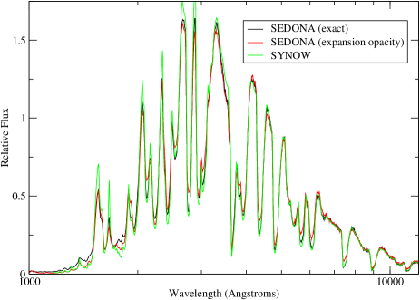
Figure 3.— SEDONA synthetic spectra of a pure silicon atmosphere compared to the output of the SYNOW code.

Lucy (2005a) discusses a simple spherically-symmetric SN Ia model used to test lightcurve calculations. The model consists of 1.4 $M_{\odot}$ of constant density ejecta extending to 10000 $\mathrm{km~{}s}^{-1}$. The ${}^{56}\mathrm{Ni}$ abundance is unity for the inner 0.5 $M_{\odot}$ of ejecta, then drops linearly to zero at 0.75 $M_{\odot}$, yielding a total ${}^{56}\mathrm{Ni}$ mass of 0.625 $M_{\odot}$. For the test calculations, a grey absorption coefficient of $\alpha/\rho=0.1$ g cm^-2 is adopted.

We have calculated a spherical SEDONA lightcurve for the model using the parameters given in the first row of Table 1. Although this problem is one of monochromatic grey radiative transfer, to fully test the MC transfer procedure and temperature solver we use 2000 opacity wavelength bins each of which is set to the same (purely absorbing) grey opacity. The results of the SEDONA calculation (Figure 1) show excellent agreement with the numerical solution of the comoving moment equations presented in Lucy (2005a). Detailed agreement obtains for both the rate of gamma-ray energy deposition from radioactive decay and the observer-frame bolometric light curve. This verifies both our gamma-ray deposition procedure and our primary MC transfer routine. The discrepancy in the light curves is comparable to the error attributed to the Eddington approximation in the comoving frame calculations by Lucy (2005a).

We have further tested the SEDONA calculations of the ejecta temperature structure using the same model. Figure 2 shows that, at all epochs, our radial temperature structure is in excellent agreement with the numerical results of Lucy (2005a). This confirms that the SEDONA MC estimators obtain the correct mean intensity of the radiation field in the time-dependent transfer calculation.

3.2. Spectrum and Polarization Tests

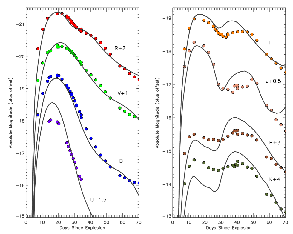
Figure 4.— SEDONA calculation of the UBVRIJHK lightcurves of the w7 Type Ia supernova explosion model. Overplotted are the Krisciunas et al. (2003) observations of SN 2001el, corrected for extinction.

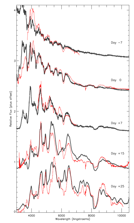
Figure 5.— SEDONA calculation of the spectra at several epochs of the w7 model compared to observations of SN 1994D. Dates given are days relative to B-band maximum.

Basic spectrum formation in SEDONA has been tested by comparing to SYNOW, a 1-D spectrum synthesis code used in many analyses of SN spectra (Branch et al., 2002, and references therein). SYNOW solves the transfer equation assuming the Sobolev approximation, time-independence, a perfectly sharp blackbody emitting photosphere, no continuum opacity, and a pure scattering line source function. Test synthetic spectra were computed with SEDONA under the same assumptions and the model parameters given in row 2 of Table 1. The particular test model discussed here consisted of pure silicon ejecta extending to 20000 $\mathrm{km~{}s}^{-1}$ with a constant density ($\rho=10^{-13}$ g/cm³) and temperature ($T=10000$ K). The photosphere was located at 10000 $\mathrm{km~{}s}^{-1}$.

Figure 3 compares the SYNOW spectrum to two SEDONA spectrum calculations – one in which the line opacity is treated directly, and another in which all the lines have been binned into the quasi-continuous expansion opacity (Eq. 6). In each case, the lines are assumed to be pure scattering – i.e. fluorescence is ignored and $\epsilon=0$.

For the direct line treatment, the agreement of the spectrum with that of SYNOW is quite good, implying a proper reproduction of the line source function for blended lines. Differences of the order a few percent are noticed, and can be attributed to the fact that different linelist data is used in the separate codes. The expansion opacity spectrum, on the other hand, does show noticeable discrepancies in the depth of individual line features. This is clearly a failure of the formalism to properly treat wavelength bins that contain only one very optically thick line ($\tau_{l}\gg 1)$. According to Eq. 6, the optical depth accrued in redshifting across such a bin is unity, and the probability of interacting with the line 1 - $\exp(-1)\approx 0.63$. This underestimates the true interaction probability $1-\exp(-\tau_{l})\approx 1$. A modification to the expansion opacity formalism to better handle this limit may be warranted.

SEDONA calculations of the emergent continuum polarization have been tested as well for a variety of cases. In the optically thin limit, we have verified the pure electron scattering polarization levels against the semi-analytical formulae of Brown & McLean (1977). In the optically thick case, we have reproduced the plane-parallel results of Chandrasekhar (1960) and those of the axisymmetric configurations calculated in Hillier (1994).

3.3. Example Application Calculations

As an example of the application of SEDONA to a realistic research problem, we calculate the spectra and lightcurves of the parameterized 1-D SN Ia explosion model w7 (Nomoto et al., 1984; Thielemann et al., 1986). Several previous radiative transfer studies using w7 have shown the model to be reasonable – but not perfect – accordance with observations (Branch et al., 1985; Harkness, 1991; Jeffery et al., 1992; Nugent et al., 1997; Lentz et al., 2001). Note that some earlier 2-D, time-independent SEDONA spectral calculations based upon w7 have already appeared (Kasen et al., 2004; Kasen & Plewa, 2005).

Figure 4 shows the synthetic UBVRIJHK lightcurves from the SEDONA calculation of w7 using the parameters in row 3 of Table 1. For these calculations we have used the Kurucz CD1 linelist containing over 40 million lines. All lines are treated in the expansion opacity two-level atom formalism with $\epsilon=1$ (i.e., no lines are given a direct fluorescence treatment). Overplotted in Figure 4 are observations of the normal Type Ia SN 2001el (Krisciunas et al., 2003) assuming a distance modulus of 31.45 and corrected for an extinction of $A_{v}=0.5,R_{v}=2.88$. The broadband model lightcurves resemble those of the observations in most regards, such as the rise times, decline rates, and peak magnitudes. A clear secondary maximum is seen in the model near-infrared IJHK bands, although it is generally stronger than the observations. These lightcurves can be compared to w7 transfer calculations using the STELLA code (Blinnikov & Sorokina, 2004), which show a similar behavior in the optical bands.

Figure 5 compares the computed w7 spectra to observations of the Type Ia SN 1994D (Patat et al., 1996; Meikle et al., 1996) at several epochs. Given the low estimated dust extinction to this object, no redding correction has been applied. While exact agreement is not to be expected, given the known limitations of the w7 model, on the whole the model well reproduces the general spectral features and colors of the observations. The overall sensible behavior suggests that time-dependent SEDONA calculations can be used to model the spectroscopic evolution of SNe over a wide time span.

At yet later times ($t_{\mathrm{exp}}\gtrsim 70$ days), SN Ia spectra become increasingly nebular, with NLTE effects and cooling by forbidden emission lines playing dominate roles. Perhaps most signficantly, at these times one expects non-thermal ionization due to the products of radioactive decay to become important once the temperature drops low enough that LTE predicts neutrality (Swartz, 1991). This physics is not included in the present version of SEDONA, and the emergent spectra and broadband lightcurves should not be expected to be accurate at the latest epochs. However, note that Branch et al. (2005) has shown, surprisingly, that resonance line scattering by permitted transitions actually does a good job of characterizing the spectrum out past $t_{\mathrm{exp}}$= 200 days.

3.4. Convergence Properties

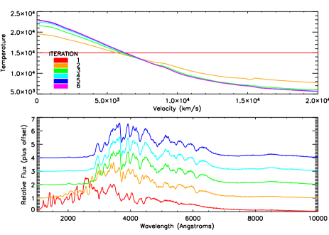
Figure 6.— Convergence of a day 18 w7 spectrum model, showing the variation of the radial temperature structure (top panel) and emergent spectrum (bottom panel) with iteration. Beginning with an isothermal temperature structure, the model converges to better than 1% in only 5 iterations.

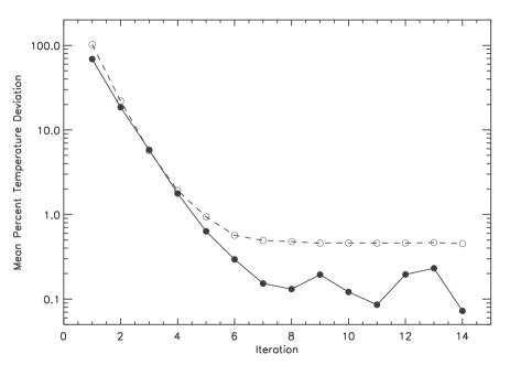
Figure 7.— Rate of convergence of the 1-D (filled circles, solid line) and 2-D (open circles, dashed line) w7-like models discussed in §3.4. The figure shows, for each iteration, the mean percent deviation of the temperature structure from that of the final iteration 15. Both models converge to better than 1% in 5 iterations, with the flattening out of the curves thereafter reflecting the level of Monte Carlo random sampling errors. The 2-D model has a larger number of cells, and thus the average sampling error in each cell is larger.

[ht]

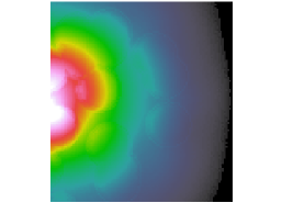
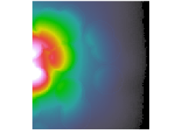
Figure 8.— Convergence of the 2-D artificial “clumpy” SN Ia model discussed in §3.4. Only the right half of the SN is shown. From left to right: Distribution of the ${}^{56}\mathrm{Ni}$ clumps; Temperature structure at iteration 2; Final converged temperature structure at iteration 15.

An issue of particular importance in radiative transfer calculations is the speed and stability of model convergence. For complicated situations – in particular time-dependent, multi-dimensional problems – convergence can be the limiting factor in the practical utility of the transfer code.

One very appealing feature of the MC approach, then, is its favorable convergence properties. Figure 6 shows the variation with iteration of the radial temperature structure at $t_{\mathrm{exp}}$= 18 days for a static spectrum calculation of the 1-D w7 model. Model parameters are those given in Table 1, row 4. All lines are treated in the expansion opacity formalism with $\epsilon=1$. Beginning with an isothermal atmosphere at T = 15000 K (a very poor initial guess, in fact) convergence is stable and rapid, with the spectrum and temperature changing negligibly after just five iterations. Figure 7 quantifies the convergence rate by showing, for each iteration, the mean percent deviation of the temperature structure from the final structure at iteration 15. After 5 iterations, the accuracy of the temperature structure is better than 1%. The flattening out of the convergence curve at $0.1\%\sim 1/\sqrt{N_{p}}$ reflects the level of random Monte Carlo sampling errors, and can only be improved by increasing the number of packets. Note that, given a more reasonable initial temperature guess (e.g., a grey atmosphere structure) the model converges (at the 1% level) to the same result after only three iterations.

The rapid convergence seen in Figure 6 highlights the utility of the constrained lambda-iteration approach developed in Lucy (1999a). In the limit that enough packets are used, the MC transfer routine always obtains the correct radiation field at all points, regardless of the dominance of scattering or NLTE line processes. Energy is strictly conserved in every packet interaction, in contrast to difference equation solutions of the radiative transfer in which energy is conserved only asymptotically as the iteration procedure converges. In the MC approach, multiple iterations are then needed only to assure that the opacities/emissivities are consistent with the temperature implied by energy balance. For problems with temperature independent opacity/emissivity, only one iteration is required. More generally, several iterations are needed, as each adjustment to the opacities feeds back into an altered radiation field structure.

Naturally, the speed of convergence hinges upon on the temperature sensitivity of the opacity. In the SNe Ia example, the dominate opacity is bound-bound line blanketing. The contribution of an individual line to the expansion opacity saturates for $\tau\gg 1$ (Equation 6), therefore the opacity is insensitive to the exact optical depth of lines, depending rather on the total number of optically thick lines. The variation with temperature is therefore smooth and gradual, contributing to the rapid and stable convergence.

These favorable convergence properties carry over to problems with complicated multi-dimensional geometries. We demonstrate this in Figure 8 using an artificial “clumpy” SN Ia model, constructed by hand to resemble multi-D deflagration models. The density structure in this 2-D example was taken from the spherical w7 model, but the 0.6 $M_{\odot}$ of ${}^{56}\mathrm{Ni}$ was randomly distributed in “clumps” (actually toruses) of velocity radius 2000 $\mathrm{km~{}s}^{-1}$. The “clumps” are surrounded by a 400 $\mathrm{km~{}s}^{-1}$ shell of silicon rich material, and are embedded in a substrate of carbon/oxygen. Model parameters are given in Table 1, row 5. Figure 7 shows that, despite the complicated and irregular geometry, the model converges as quickly as the 1-D case to better than 1% in only 5 iterations. Because of the larger number of cells in the 2-D model, however, a larger number of packets are needed to achieve adequate statistics in each cell. Figure 8 shows that the final converged temperature structure is itself highly irregular, bearing the marks of the enhanced radioactive energy generation and ionization in the ${}^{56}\mathrm{Ni}$ clumps. Similarly rapid convergence behavior is found for models exhibiting global asphericity in the density contours (Kasen et al., 2004).

3.5. Time Dependent Versus Stationary Spectrum Calculations

Many SN spectral synthesis codes to date have not explicitly included time-dependence, adopting rather a stationarity approximation. From a formal point of view, the assumption is inappropriate at early times, when the photon diffusion time ($t_{d}$) is long compared to the expansion time ($t_{\mathrm{exp}}$) of the supernova. SEDONA allows us to test the validity of the approximation in practice.

SEDONA calculations can be run in a time-independent, “snapshot” mode, such that photons are emitted according to the instantaneous radioactive deposition function, and do not diffuse in time. As an example, we compute snapshot spectra of w7 at 10 days and 18 days after explosion, for which the electron scattering diffusion times are $t_{d}=1.2$ $t_{\mathrm{exp}}$ and 0.3 $t_{\mathrm{exp}}$, respectively. The emergent bolometric luminosity is a free parameter in the snapshot calculations, which in this case was taken from the time-dependent w7 calculation discussed in §3.3.

Figure 9 compares the snapshot spectra to those of the full time-dependent calculation. The agreement is surprisingly good for both day 18 and day 10. Thus, although the time-dependent calculations include diffuse photon packets emitted at earlier epochs, the initial spectral energy distribution of such packets has apparently been erased during the transfer. Wavelength redistribution processes operate on each packet on a short enough time scale such that the original time of emission of a photon packet is not an important factor.

We conclude that, at least in the context 1-D SN Ia calculations, stationarity is a very reasonable approximation near and even prior to maximum light. The major limitation of the approximation, of course, is its inability to predict the emergent bolometric luminosity at any given time, which must therefore be included as a free parameter in the simulation. Stationarity may also be more questionable in multi-dimensional polarization calculations, for which the directional diffusion time and isotropy of the radiation field is of importance.

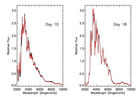
Figure 9.— Comparison of time-dependent spectral calculations (thick, black lines) to time-independent “snapshot” calculations (thin red,lines) for the w7 model at days $t_{\mathrm{exp}}$=10 and 18.

3.6. Fluorescence Versus Two-Level Atom Redistribution

For SN spectral calculations, the wavelength redistribution of photons in bound-bound transitions constitutes an essential component of the radiative transfer. In SNe Ia, for example, photon packets are typically initiated in the hot, inner regions of ejecta, where the thermal emissivity peaks in the ultraviolet (UV). The opacity in the UV is large due to high density of Fe-peak lines, and the diffusion time of UV photons exceedingly long. Photon escape, however, is greatly enhanced by interactions with lines, which degrade photons to redder wavelengths, where the opacity is lower. The primary method by which this occurs is fluorescence (a.k.a. line-splitting)– i.e., a UV photon excites an high-energy atomic transition, followed by de-excitation via a redder transition (Pinto & Eastman, 2000b).

Obviously a proper treatment of the wavelength redistribution in lines is critical for calculating the lightcurves of SNe. As previously discussed (§2.3.2), SEDONA allows for a direct MC treatment of line fluorescence. The approach, however, places sizeable computational and memory demands on a system, and is usually only feasible when using a restricted linelist ($\lesssim 500,000$ lines). A simpler, approximate method is desirable, and so in §2.2 we introduced the two-level atom (TLA) expansion opacity approach. Here lines either scatter or “absorb” radiation, depending upon the assigned redistribution probability parameter $\epsilon$. Absorption in a line is followed by immediate re-emission in another line according to a thermal distribution, a process which is designed to mimic fluorescence (the probability of true absorption is in fact very small).

Here we explore how well a simple constant $\epsilon$ TLA approach approximates the true wavelength redistribution calculated with line-fluorescence treated directly. We compute spectra and lightcurves of the w7 model using both methods, applying a linelist of nearly 500,000 lines from the Kurucz CD 23. In one test calculation, all 500,000 lines are given a direct fluorescence treatment. In the other test calculations, all 500,000 lines are treated using the expansion opacity TLA formalism with different values of the redistribution probability $\epsilon$. We explore three values of $\epsilon$, viz., $1.0,0.3$, and $0.01$.

Figure 10 compares stationary w7 spectra computed near maximum light ($t_{\mathrm{exp}}$= 18 days). For high redistribution probability ($\epsilon=1$ or $0.3$) the TLA approach in fact reasonably approximates the line-fluorescence spectrum. In the example, the $\epsilon=1$ model somewhat overestimates the redistribution, moving too much flux to the red, while the $\epsilon=0.3$ calculation more accurately reproduces the colors. The scattering dominated atmosphere ($\epsilon=0.01$), on the other hand, dramatically fails to properly redistribute flux, leading to unreasonable results. Similar behavior was found by Nugent et al. (1997).

The synthetic light curves in Figure 11 demonstrate that essentially the same effect operates in the time-dependent calculation. For $\epsilon>0.1$, the TLA bolometric lightcurves are remarkably similar to the line-fluorescence calculations. Discrepancies are naturally larger in the monochromatic lightcurves, which are more sensitive to the redistribution. For example, the $\epsilon=1$ and $\epsilon=0.3$ B-band lightcurves are slightly depressed at peak, as too much flux is moved to the red (the R and I band lightcurves are correspondingly brighter). The $\epsilon=0.01$ atmosphere, however, gives completely unreasonable results. In the absence of sufficient redistribution, packets are frozen at the high-opacity UV wavelengths. Diffusion times are long and adiabatic losses severe. This emphasizes the critical importance of wavelength redistribution via fluorescence in the lightcurves of SNe Ia (Pinto & Eastman, 2000b).

Overall, the TLA approach offers a useful approximation for many lightcurve and spectral studies of interest. In the present example, the errors in the B-band lightcurve are of order 0.1 mag, probably comparable to other uncertainties in the transfer calculation. Moreover, the output is not particularly sensitive to the value of $\epsilon$, as long as $\epsilon$ is close to unity. The effectiveness of the TLA approach is not entirely surprising. Given the extreme complexity of the iron-peak element’s atomic structure and the high rate of packet-line interactions, a quasi-equilibrium is nearly established and assuming thermal redistribution in fact fairly well represents the actual fluorescence processes.

One could improve the TLA approximation somewhat by calibrating $\epsilon$ for each line individually in an effort to better reproduce the line source functions (e.g. Höflich, 1995). We note that in the present context, the redistribution probability for a given atomic transition between lower level $l$ and upper level $u$ can be approximated as

$$p_{\mathrm{fluor}}=\frac{\sum_{k\neq l}\beta_{uk}A_{uk}}{N_{e}\sum_{k}C_{uk}+\sum_{k}\beta_{uk}A_{uk}}.$$ (41)

This formula expresses the probability that the radiative excitation $l\rightarrow u$ is followed by de-excitation into a lower level other than $l$. For the conditions in SNe Ia, one finds that for most lines $p_{\mathrm{fluor}}=0.1-1.0$. To eliminate altogether the free $\epsilon$ parameter occurring in our TLA approach, one could take $\epsilon=p_{\mathrm{fluor}}$ where $p_{\rm fluor}$ is computed using Equation 41 for each line individually and for the specific ejecta conditions in each spatial cell and time. Because $p_{\rm fluor}$ is found typically to be near unity, transfer calculations using this approach will not in fact differ much from the constant $\epsilon=1$ and $\epsilon=0.3$ calculations demonstrated in this section.

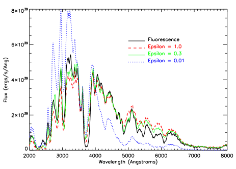
Figure 10.— Spectra of the w7 model (at day 18) calculated using a direct treatment of line fluorescence (black line) compared to the TLA approach with various redistribution probabilities (colored lines).

Figure 11.— Bolometric and B-band lightcurve of the w7 model calculated using a direct treatment of line fluorescence (black line) compared to the TLA approach with various redistribution probabilities (colored lines).

4. Summary and Conclusions

In this paper we have described the computational techniques, and demonstrated applications and verifications of the multi-dimensional MC transfer code SEDONA. We have also explored the validity of several common approximations made in SN transfer models. These findings will be drawn upon in future applications of the code.

Although computational efficiency is often considered a drawback of MC codes, the effective parallelization and favorable convergence properties of the present techniques allow SEDONA to immediately address complicated transfer problems using currently available computing resources. Moreover, as the physics included in the radiative transfer simulation becomes increasingly complicated, including all of multi-dimensionality, NLTE effects, polarization and time-dependence, it is not clear that difference equation techniques will outperform MC approaches in their execution times.

With further work, and with the advance of computing power, some of the presently applied approximations can be relaxed. Most outstanding is the inclusion of an NLTE treatment of the occupation numbers, including excitation/ionization by non-thermal electrons scattered from radioactive gamma-rays. Inclusion of nebular physics and cooling by forbidden line transitions would also improve model accuracy at late times. Eventually, coupling of the transfer code to a multi-dimensional hydrodynamical solver would allow the calculations to be generalized to non-homologous flows. Fortunately, the foreseeable improvements are readily incorporated into the MC framework in a straightforward and intuitive manner.

Appendix A Gamma-Ray Transfer

Several discussions of MC gamma-ray transfer calculations for SN can be found in the literature, including Swartz et al. (1995), Höflich et al. (1994), Ambwani & Sutherland (1988), Milne et al. (2004), and references therein. The important opacities for gamma-rays are Compton scattering and photoelectric absorption (the additional opacity due to pair-production is typically small and will be ignored). Because the gamma-ray energies are much greater than the atomic binding energies, all electrons in an atom (bound and free) contribute to the Compton opacity, which for a gamma-ray packet of energy $E_{\gamma}$ is

$$\alpha_{\mathrm{c}}=\sigma_{\mathrm{T}}NK(x)\sum_{i}X_{i}Z_{i},$$ (A1)

where $x=E_{\gamma}/m_{e}c^{2}$, $\sigma_{T}$ is the Thomson cross-section, and $N$ is the total number density. The sum runs over all elements with abundance fraction by number $X_{i}$ and atomic number $Z_{i}$. The dimensionless quantity $K(x)$ is the Klein-Nishina correction to the cross-section

$$K(x)=\frac{3}{4}\biggl{[}\frac{1+x}{x^{3}}\biggl{(}\frac{2x(1+x)}{1+2x}-\ln(1+2x)\biggr{)}+\frac{1}{2x}\ln(1+2x)-\frac{1+3x}{(1+2x)^{2}}\biggr{]}.$$ (A2)

$K(x)$ is always less than one and decreases with increasing x.

Typically Compton opacity dominates for $E_{\gamma}\gtrsim 50$ keV, while photoelectric absorption dominates for lower energies. The photoelectric extinction coefficient is dominated by the two K-shell electrons, and can be approximated as

$$\alpha_{\mathrm{p}}=\sigma_{\mathrm{T}}\alpha^{4}8\sqrt{2}x^{-7/2}N\sum_{i}Z_{i}^{5}X_{i},$$ (A3)

where $\alpha$ is the fine-structure constant.

Individual gamma-ray packets are emitted proportional to the local decay rate of radioactive nuclei in one of several gamma-ray lines, listed, for example, in Ambwani & Sutherland (1988). The energy of each packet is initially $E_{\gamma}=E_{\rm rad,tot}/N_{\gamma}$, where $E_{\rm rad,tot}$ is the total gamma-ray energy emitted from radioactive decay and $N_{\gamma}$ the number of packets used in the simulation. The gamma-ray packets are tracked through scatterings and absorptions through the atmosphere much as described for the optical packets in §2.3.2, with the propagation coming to an end when the packet either escapes the atmosphere or is photo-absorbed in the ejecta.

In a Compton scattering, a new direction for the gamma-ray is sampled from the anisotropic differential cross-section

$$\frac{d\sigma}{d\Omega}=\frac{3\sigma_{T}}{16\pi}f(x,\Theta)^{2}\biggl{(}f(x,\Theta)+f(x,\Theta)^{-1}-\sin^{2}\Theta\biggr{)},$$ (A4)

where $\Theta$ is the angle between incoming and outgoing gamma-ray directions and $f(x,\Theta)$ is the ratio of incoming to outgoing gamma-ray energy,

$$f(x,\Theta)=\frac{E_{\mathrm{out}}}{E_{\mathrm{in}}}=\frac{1}{1+x(1-\cos\Theta)}.$$ (A5)

The average energy lost in an interaction is given by

$$F(x)=1-\frac{1}{4\pi}\oint d\mu d\phi\frac{d\sigma}{d\Omega}f(x,\mu).$$ (A6)

For a 1 MeV gamma-ray, $F(x)\approx 0.6$. Thus a gamma-ray loses almost all of its energy after just a few Compton scatterings, after which it will be destroyed by photo-absorption. The lost gamma-ray energy becomes the kinetic energy of fast scattered electrons, which are assumed to be thermalized locally through electron-electron collisions.

The rate of energy deposition $\dot{E}^{i,j}_{\mathrm{dep}}$ in each cell $i$ and each time step $j$ can be estimated by tallying up the gamma-ray energy lost during each scattering or absorption event. In this case, however, enough packets must be used such that many interactions occur in every cell. On a 3-D grid, this requires a very large number of packets, especially at later times when interaction events become infrequent. Fortunately, we can derive a better estimator of $\dot{E}^{i,j}_{\mathrm{dep}}$ by considering the analytic expression for the absorbed energy,

$$\dot{E}^{i,j}_{\mathrm{dep}}=\oint\int\alpha_{\mathrm{abs}}I_{\lambda}d\lambda d\Omega=4\pi\int J_{\lambda}[\alpha_{\mathrm{c}}(x)F(x)+\alpha_{\mathrm{p}}(x)]d\lambda.$$ (A7)

The mean intensity of the radiation field $J_{\lambda}$ can always be better estimated than $\dot{E}^{i,j}_{\mathrm{dep}}$ can be by direct counting of energy loses, because every packet passing through a cell contributes, regardless of whether an interaction occurs. To derive the needed estimator, we begin with the relationship between $J_{\lambda}$ and the monochromatic energy density $u_{\lambda}$ (Mihalas, 1978),

$$u_{\lambda}d\lambda=\frac{4\pi}{c}J_{\lambda}d\lambda.$$ (A8)

When a packet possessing a fraction $E/E_{\gamma}$ of its initial energy takes a velocity step of size $\Delta v_{k}$ in a cell, its contribution to $u_{\lambda}$ is

$$du_{\lambda}{d\lambda}=\frac{E_{\gamma}}{V_{i}}\biggl{(}\frac{E}{E_{\gamma}}\biggl{)}\biggl{(}\frac{\delta t}{\Delta y}\biggr{)},$$ (A9)

where $V_{i}$ is the volume of the cell, $\Delta t$ the size of the time slice, and $\delta t=\Delta v_{k}~{}t_{\mathrm{exp}}/c$. Using this equation and Equation A7 gives

$$\dot{E}^{i,j}_{\mathrm{dep}}=\frac{E_{\gamma}}{V_{i}~{}\Delta t}\sum_{k}(\Delta v_{k}~{}t_{\mathrm{exp}})\frac{E}{E_{\gamma}}\biggl{[}\alpha_{\mathrm{c}}(x)F(x)+\alpha_{\mathrm{p}}(x)\biggr{]},$$ (A10)

where the sum over $k$ runs over every packet step that occurs inside the cell.

Note that because the gamma-ray opacities are independent of temperature, the gamma-ray transfer procedure need not be repeated at every iteration. Rather $\dot{E}^{i,j}_{\mathrm{dep}}$ need only be computed once and stored at the beginning of a run.

References

- Ambwani & Sutherland (1988) Ambwani, K. & Sutherland, P. 1988, ApJ, 325, 820
- Auer (2003) Auer, L. 2003, in Stellar Atmosphere Modeling, Proceedings of an International Workshop held in Tübingen, Germany, 8-12 April 2002, ed. D. M. Ivan Hubeny & K. Werner (Astronomical Society of the Pacific), 3
- Baron et al. (1996) Baron, E., Hauschildt, P. H., & Mezzacappa, A. 1996, MNRAS, 278, 763
- Blinnikov & Sorokina (2004) Blinnikov, S. & Sorokina, E. 2004, Ap&SS, 290, 13
- Branch et al. (2005) Branch, D., Baron, E., Hall, N., Melakayil, M., & Parrent, J. 2005, PASP, 117, 545
- Branch et al. (2002) Branch, D., Benetti, S., Kasen, D., Baron, E., Jeffery, D. J., Hatano, K., Stathakis, R. A., Filippenko, A. V., Matheson, T., Pastorello, A., Altavilla, G., Cappellaro, E., Rizzi, L., Turatto, M., Li, W., Leonard, D. C., & Shields, J. C. 2002, ApJ, 566, 1005
- Branch et al. (1985) Branch, D., Doggett, J. B., Nomoto, K., & Thielemann, F.-K. 1985, ApJ, 294, 619
- Brown & McLean (1977) Brown, J. C. & McLean, I. S. 1977, A&A, 57, 141
- Burrows et al. (1995) Burrows, A., Hayes, J., & Fryxell, B. 1995, ApJ, 450, 830
- Castor (1970) Castor, J. I. 1970, MNRAS, 149, 111
- Chandrasekhar (1960) Chandrasekhar, S. 1960, Radiative Transfer (New York: Dover, 1960)
- Chevalier & Klein (1978) Chevalier, R. A. & Klein, R. I. 1978, ApJ, 219, 994
- Code & Whitney (1995) Code, A. D. & Whitney, B. A. 1995, ApJ, 441, 400
- Cropper et al. (1988) Cropper, M., Bailey, J., McCowage, J., Cannon, R. D., & Couch, W. J. 1988, MNRAS, 231, 695
- Cunto & Mendoza (1992) Cunto, W. & Mendoza, C. 1992, Revista Mexicana de Astronomia y Astrofisica, vol. 23, 23, 107
- Daniel (1980) Daniel, J. Y. 1980, A&A, 86, 198
- Decourchelle et al. (2001) Decourchelle, A. et al. 2001, A&A, 365, L218
- Eastman & Pinto (1993) Eastman, R. G. & Pinto, P. A. 1993, ApJ, 412, 731
- Fesen & Gunderson (1996) Fesen, R. & Gunderson, K. 1996, ApJ, 470, 967
- Gamezo et al. (2003) Gamezo, V. N., Khokhlov, A. M., Oran, E. S., Chtchelkanova, A. Y., & Rosenberg, R. O. 2003, Science, 299, 77
- Hamilton (1947) Hamilton, D. R. 1947, ApJ, 106, 457
- Hanuschik & Dachs (1987) Hanuschik, R. W. & Dachs, J. 1987, A&A, 182, L29+
- Harkness (1991) Harkness, R. 1991, in Supernova 1987A and other supernovae, ESO Conference and Workshop Proceedings, Proceedings of an ESO/EIPC Workshop, Marciana Marina, Isola d’Elba, September 17-22, 1990, Garching: European Southern Observatory (ESO), edited by I. J. Danziger, and Kurt Kjär., p 447
- Herant & Woosley (1994) Herant, M. & Woosley, S. E. 1994, ApJ, 425, 814
- Hillier (1994) Hillier, D. J. 1994, A&A, 289, 492
- Höflich (1991) Höflich, P. 1991, A&A, 246, 481
- Höflich (1995) Hoflich, P. 1995, ApJ, 443, 89
- Höflich (2002) Höflich, P. 2002, New Astronomy Review, 46, 475
- Höflich et al. (1994) Hoeflich, P., Khokhlov, A., & Mueller, E. 1994, ApJS, 92, 501
- Höflich et al. (1996) Höflich, P., Wheeler, J. C., Hines, D. C., & Trammell, S. R. 1996, ApJ, 459, 307
- Howell et al. (2001) Howell, D. A., Höflich, P., Wang, L., & Wheeler, J. C. 2001, ApJ, 556, 302
- Hungerford et al. (2003) Hungerford, A. L., Fryer, C. L., & Warren, M. S. 2003, ApJ, 594, 390
- Hwang et al. (2000) Hwang, U., Holt, S., & Petre, R. 2000, ApJ, 537, L119
- Jeffery (1989) Jeffery, D. J. 1989, ApJS, 71, 951
- Jeffery (1995) Jeffery, D. J. 1995, A&A, 299, 770
- Jeffery & Branch (1990) Jeffery, D. & Branch, D. 1990, in Supernovae, Jerusalem Winter School for Theoretical Physics, ed. S. W. J.C. Wheeler, T. Piran (World Scientific Publishing Co.), 149
- Jeffery et al. (1992) Jeffery, D. J., Leibundgut, B., Kirshner, R. P., Benetti, S., Branch, D., & Sonneborn, G. 1992, ApJ, 397, 304
- Karp et al. (1977) Karp, A. H., Lasher, G., Chan, K. L., & Salpeter, E. E. 1977, ApJ, 214, 161
- Kasen et al. (2004) Kasen, D., Nugent, P., Thomas, R. C., & Wang, L. 2004, ApJ, 610, 876
- Kasen & Plewa (2005) Kasen, D. & Plewa, T. 2005, ApJ, 622, L41
- Kawabata et al. (2002) Kawabata, K. S. et al. 2002, ApJ, 580, L39
- Khokhlov et al. (1999) Khokhlov, A. M., Höflich, P. A., Oran, E. S., Wheeler, J. C., Wang, L., & Chtchelkanova, A. Y. 1999, ApJ, 524, L107
- Kifonidis et al. (2000) Kifonidis, K., Plewa, T., Janka, H.-T., & Müller, E. 2000, ApJ, 531, L123
- Krisciunas et al. (2003) Krisciunas, K., Suntzeff, N. B., Candia, P., Arenas, J., Espinoza, J., Gonzalez, D., Gonzalez, S., Höflich, P. A., Landolt, A. U., Phillips, M. M., & Pizarro, S. 2003, AJ, 125, 166
- Kurucz & Bell (1995) Kurucz, R. L. & Bell, B. 1995, Atomic line list (Kurucz CD-ROM, Cambridge, MA: Smithsonian Astrophysical Observatory, —c1995, April 15, 1995)
- Lentz et al. (2001) Lentz, E. J., Baron, E., Branch, D., & Hauschildt, P. H. 2001, ApJ, 557, 266
- Leonard et al. (2005) Leonard, D. C., Li, W., Filippenko, A. V., Foley, R. J., & Chornock, R. 2005, ApJ, 632, 450
- Li & McCray (1993) Li, H. & McCray, R. 1993, ApJ, 405, 730
- Lucy (1999a) Lucy, L. B. 1999a, A&A, 344, 282
- Lucy (1999b) —. 1999b, A&A, 345, 211
- Lucy (2001) —. 2001, MNRAS, 326, 95
- Lucy (2002) —. 2002, A&A, 384, 725
- Lucy (2003) —. 2003, A&A, 403, 261
- Lucy (2005a) —. 2005a, A&A, 429, 19
- Lucy (2005b) —. 2005b, A&A, 429, 31
- MacFadyen & Woosley (1999) MacFadyen, A. I. & Woosley, S. E. 1999, ApJ, 524, 262
- Marietta et al. (2000) Marietta, E., Burrows, A., & Fryxell, B. 2000, ApJS, 128, 615
- Mazzali et al. (1995) Mazzali, P. A., Danziger, I. J., & Turatto, M. 1995, A&A, 297, 509
- Mazzali & Lucy (1993) Mazzali, P. A. & Lucy, L. B. 1993, A&A, 279, 447
- Mazzali et al. (2001) Mazzali, P. A., Nomoto, K., Patat, F., & Maeda, K. 2001, ApJ, 559, 1047
- Meikle et al. (1996) Meikle, W. P. S. et al. 1996, MNRAS, 281, 263
- Mihalas (1978) Mihalas, D. 1978, Stellar Atmospheres (San Francisco: W. H. Freeman)
- Milne et al. (2004) Milne, P. A., Hungerford, A. L., Fryer, C. L., Evans, T. M., Urbatsch, T. J., Boggs, S. E., Isern, J., Bravo, E., Hirschmann, A., Kumagai, S., Pinto, P. A., & The, L.-S. 2004, ApJ, 613, 1101
- Nomoto et al. (1984) Nomoto, K., Thielemann, F., & Yokoi, K. 1984, ApJ, 286, 644
- Nugent et al. (1997) Nugent, P., Baron, E., Branch, D., Fisher, A., & Hauschildt, P. H. 1997, ApJ, 485, 812
- Patat et al. (1996) Patat, F. et al. 1996, MNRAS, 278, 111
- Pinto & Eastman (2000a) Pinto, P. A. & Eastman, R. G. 2000a, ApJ, 530, 744
- Pinto & Eastman (2000b) —. 2000b, ApJ, 530, 757
- Plewa et al. (2004) Plewa, T., Calder, A. C., & Lamb, D. Q. 2004, ApJ, 612, L37
- Röpke (2005) Röpke, F. K. 2005, A&A, 432, 969
- Röpke & Hillebrandt (2005) Röpke, F. K. & Hillebrandt, W. 2005, A&A, 431, 635
- Rybicki & Lightman (1986) Rybicki, G. B. & Lightman, A. P. 1986, Radiative Processes in Astrophysics (Radiative Processes in Astrophysics, by George B. Rybicki, Alan P. Lightman, pp. 400. ISBN 0-471-82759-2. Wiley-VCH , June 1986.)
- Sobolev (1947) Sobolev, V. V. 1947, Moving Envelopes of Stars (Leningrad: Leningrad State University)
- Swartz (1991) Swartz, D. A. 1991, ApJ, 373, 604
- Swartz et al. (1995) Swartz, D. A., Sutherland, P. G., & Harkness, R. P. 1995, ApJ, 446, 766
- Thielemann et al. (1986) Thielemann, F.-K., Nomoto, K., & Yokoi, K. 1986, A&A, 158, 17
- Utrobin et al. (1995) Utrobin, V., Chugai, N., & Andronova, A. 1995, A&A, 295, 129
- van Regemorter (1962) van Regemorter, H. 1962, ApJ, 136, 906
- Wang et al. (2003) Wang, L., Baade, D., Höflich, P., Khokhlov, A., Wheeler, J. C., Kasen, D., Nugent, P. E., Perlmutter, S., Fransson, C., & Lundqvist, P. 2003, ApJ, 591, 1110
- Wang et al. (1997) Wang, L., Wheeler, J. C., & Hoeflich , P. 1997, ApJ, 476, L27
- Wood et al. (1996) Wood, K., Bjorkman, J. E., Whitney, B. A., & Code, A. D. 1996, ApJ, 461, 828
- Yoon & Langer (2005) Yoon, S.-C. & Langer, N. 2005, A&A, 435, 967
- Zhang & Wang (1996) Zhang, Q. & Wang, Z. R. 1996, A&A, 307, 166