The role of Kelvin-Helmholtz instability in the internal structure of relativistic outflows. The case of the jet in 3C 273

Abstract

Context. Relativistic outflows represent one of the best-suited tools to probe the physics of AGN. Numerical modelling of internal structure of the relativistic outflows on parsec scales provides important clues about the conditions and dynamics of the material in the immediate vicinity of the central black holes in AGN.

Aims. We investigate possible causes of the structural patterns and regularities observed in the parsec-scale jet of the well-known quasar 3C 273.

Methods. We present here the results from a 3D relativistic hydrodynamics numerical simulation based on the parameters given for the jet by Lobanov & Zensus (2001), and one in which the effects of jet precession and the injection of discrete components have been taken into account. We compare the model with the structures observed in 3C 273 using very long baseline interferometry and constrain the basic properties of the flow.

Results. We find growing perturbation modes in the simulation with similar wavelengths to those observed, but with a different set of wave speeds and mode identification. If the observed longest helical structure is produced by the precession of the flow, longer precession periods should be expected.

Conclusions. Our results show that some of the observed structures could be explained by growing Kelvin-Helmholtz instabilities in a slow moving region of the jet. However, we point towards possible errors in the mode identification that show the need of more complete linear analysis in order to interpret the observations. We conclude that, with the given viewing angle, superluminal components and jet precession cannot explain the observed structures.

1 Introduction

The structure and kinematics of parsec-scale outflows is typically explained in terms of shocks (Marscher mar80 (1980), Marscher & Gear mg85 (1985), Gómez et al. gam93 (1993), gam94 (1994), Gómez et al. gom+94 (1994)) and Kelvin-Helmholtz (K-H) instabilities (Hardee har82 (1982), har84 (1984), har87 (1987), Hardee et al. hcr97 (1997), Hardee har00 (2000), har03 (2003), Hardee et al. har05 (2005)) developing in a relativistic fluid. Relativistic shocks may dominate the jet dynamics and emission at small scales, but are likely to dissipate at distances larger than $\sim 10$ pc (Lobanov & Zensus lz99 (1999)) due to the interaction with the slower flow. On intermediate scales ($\sim 10$–100 pc) shocks and plasma instabilities may play equally important roles in jets (Lobanov & Roland lr01 (2001)). Distributions of the synchrotron turnover frequency obtained for 3C 273 (Lobanov et al. 1997) and 3C 345 (Lobanov 1998) indicate that both shocks and instabilities are present on these scales, while larger scales are most likely dominated by plasma instabilities alone.

Recent studies by Hardee (har00 (2000)) have shown that K-H instability may produce complex, three-dimensional ribbon-like and thread-like patterns inside a relativistic jet. In these ribbons and threads, a substantial increase of particle pressure and radio emissivity can be expected. This model has been successfully applied to the jet in 3C 120 (Hardee har03 (2003), Hardee et al. har05 (2005)). The threaded structure forming a double helix has been detected in a space VLBI image of 3C 273 made at 5 GHz (Lobanov et al. lob+00 (2000)). It was explained in terms of K-H instability developing in a relativistic flow with a modest Lorentz factor $\gamma=2.1$ and a relativistic Mach number $M=3.5$ (Lobanov & Zensus 2001, hereafter LZ (01)). The analytical approach used in LZ01 is based on linear perturbation analysis of a K-H instability developed by Hardee (har87 (1987), har00 (2000)). A similar approach applied to kiloparsec-scale jet in M87 allowed for accurate determination of physical parameters and modelling of radio emission to be made (Lobanov et al. lhe03 (2003)).

However, results from numerical simulations of relativistic flows indicate that, after the linear regime of instability growth, the jets can be easily disrupted (Perucho et al. 2004b ). In addition to this, the bulk Lorentz factor $\gamma=2.1$ derived in LZ01 is below the values required to explain the apparent speeds of $\beta_{\mathrm{app}}\sim 5-8\,c$ of enhanced emission features observed in 3C 273. LZ01 suggest that the K-H instability is developing in a slower, underlying flow, and the fast components are most likely faster shock waves produced in the jet by the periodic ejections associated with the nuclear flares. The presence of such shocks may disrupt the linear growth of the K-H instability as well, and it is not clear whether the linear stability analysis can be still applied in the presence of these kind of non-linear effects in the flow.

In view of these concerns, it is important to confront the results of LZ01 with numerical simulations, and attempt to address several fundamental issues about the stability and propagation of relativistic flows similar to the one observed in 3C 273. Numerical simulations can be used to verify whether the linear theory can be applied for explaining self-consistently the morphology and kinematics of parsec-scale flows, and whether these flows preserve fingerprints of linear modes even when the non-linear regime has developed or non-linear features, such as fast components, appear. Numerical simulations provide a means to address these problems by following the transition from linear to non-linear regimes of instability development (Perucho et al. 2004a ; 2004b ). The ultimate goal of this work is to probe the advantages and limitations of the combination of different approaches (linear theory, numerical simulations and observations) to studies of parsec-scale jets.

3C 273 is the second quasar discovered (Hazard et al. hms63 (1963)), and the first one for which the emission lines were identified with red-shifted hydrogen lines (Schmidt sch63 (1963)). In the same work, Schmidt (sch63 (1963)) also pointed out the presence of a jet-like structure in this object. During the last four decades, the active nucleus and the relativistic outflow in 3C 273 have been studied in great detail (Courvoisier cou98 (1998)). The parsec-scale radio jet in 3C 273 has been monitored for almost three decades (Pearson et al. pea+81 (1981), Unwin et al. unw+85 (1985), unw+89 (1989), Zensus et al. zen+88 (1988), zen+90 (1990), Davis et al. dum91 (1991), Abraham et al. abr+96 (1996), Krichbaum et al. kwz00 (2000), Lobanov et al. lob+00 (2000), Asada et al. asa+02 (2002)). The emission associated with the relativistic outflow on kiloparsec scales has been probed extensively in the radio (Conway et al. con+81 (1981), con+93 (1993)), near infrared (Neumann et al. nmr97 (1997), Hutchings et al. hut+04 (2004)), optical (Thompson et al. tmw93 (1993), Jester jes01 (2001), Jester et al. jes+01 (2001)) and X-ray (Röser et al. roe+00 (2000), Marshall et al. mar+01 (2001), Sambruna et al. sam+01 (2001)) wavebands.

The relativistic jet observed in the quasar 3C273 is one-sided, with no signs of emission on the counter-jet side at dynamic ranges of up to 16,000:1 (Unwin et al. unw+85 (1985)). This is evidence for strong relativistic boosting in an intrinsically double-sided outflow powered by an accretion disk around the central black hole (Begelman et al. bbr84 (1984)). The mass of the central black hole in 3C 273 is estimated to be $M_{\mathrm{bh}}=5.5^{+0.9}_{-0.8}\times 10^{8}\mathrm{M}_{\sun}$ (Kaspi et al. kas+00 (2000)). The enhanced emission features (jet components) identified in the jet on scales of up to $\sim$20 milliarcseconds (mas) are moving at apparent speeds exceeding the speed of light by factors of 5-8 (Abraham et al. abr+96 (1996)). Plausible ranges of the Lorentz factor $\gamma\approx 5$–10 and viewing angles $\theta_{\mathrm{jet}}\approx 10\degr$–$15\degr$ have been inferred from these measurements.

Ejections of new components into the jet occur roughly once every year (Krichbaum et al. kwz00 (2000)), and they are likely to be related to weak optical flares observed with a similar periodicity (Belokon bel81 (1981)). The position angle at which the components are ejected shows regular variations with a likely period of about 13–15 years (Abraham et al. abr+96 (1996), Abraham & Romero ar99 (1999)), correlated with the long-term variability observed in 3C 273 in the optical (Babadzhanyants & Belokon bb93 (1993)) and radio (Turler et al. tcp99 (1999)) bands. Abraham & Romero (ar99 (1999)) have suggested that this periodicity may reflect changes of the jet axis induced by the relativistic precession of the inner part of the accretion disk.

Results from the linear analysis and numerical modelling are presented, compared and discussed in Sect. 2 in connection to explaining the observed properties of parsec-scale outflow in 3C 273. Main results of the work are discussed in Sect. 3.

Throughout the paper, we adopt the flat $\Lambda$CDM Cosmology with the Hubble constant $H_{0}=71\,h\,$km  s^-1 Mpc^-1, where $h$ is a constant with a likely value of 1, and matter density $\Omega_{M}=0.27$. The positive definition of spectral index, $S\propto\nu^{\alpha}$ is used. For 3C 273 ($z=0.157$, Strauss et al. str+92 (1992)), the adopted cosmological parameters correspond to the luminosity distance $D_{\mathrm{L}}=0.7h^{-1}$ Gpc. The respective linear scale is $2.69h^{-1}$ pc mas^-1, and a proper motion of 1 mas/yr corresponds to an apparent speed of $10.1h^{-1}\,c$.

2 Numerical simulations

In this section, we present numerical simulations performed with the aim to provide a counterpart to the analytical modelling of the jet structure in 3C 273 made in LZ01. To give a better account of the connection between the analytical and numerical approaches, basic results from the linear model of LZ01 are briefly summarized below.

2.1 Results from the linear analysis

Linear perturbation analysis of Kelvin-Helmholtz instability (cf. Hardee har87 (1987, 2000) and Hardee et al. hcr97 (1997)) was applied in LZ01 to explaining the internal structure of the jet in 3C 273. The locations of two thread-like features identified inside the jet (the features P1 and P2, in the nomenclature of LZ01) were approximated by combinations of several oscillatory modes. These modes were identified with different modes of Kelvin-Helmholtz instability. The parameters of these modes are given in Table 1. The characteristic wavelengths of different instability modes can be related to the jet speed ($\beta_{j}$), Mach number ($M_{j}$) and the density ratio ($\eta=\rho_{j}/\rho_{a}$) between the jet and the ambient medium. These wavelengths are obtained by approximating the dispersion relation in the small frequency limit ($\omega\rightarrow 0$) and large frequency limit ($\omega\gg$). Both are obtained for highly supersonic jets ($M_{j}\gg 1$). The longest unstable wavelength, $\lambda^{l}_{nm}$ (obtained in the low-frequency limit), and the resonant wavelength, $\lambda^{*}_{nm}$ (obtained in the high frequency limit), are given by (Hardee har87 (1987)):

$$\lambda^{l}_{nm}=\frac{4\gamma_{j}R_{j}(M_{j}^{2}-1)^{1/2}}{n+2m-1/2}\,,$$ (1)

$$\lambda^{*}_{nm}=\frac{2\pi}{\beta_{s,a}/\beta_{j}\,(n+m+1/2)}$$

$$\qquad\qquad\qquad\frac{\gamma_{j}(M_{j}^{2}-\beta_{j}^{2})^{1/2}}{(M_{a}^{2}-\beta_{j}^{2})^{1/2}+\gamma_{j}(M_{j}^{2}-\beta_{j}^{2})^{1/2}}\,,$$ (2)

where $\beta_{s,a}$ is the sound speed of the external medium in units of the speed of light, $\gamma_{j}$ is the Lorentz factor of the jet, $M_{a}=\beta_{j}/\beta_{s,a}$, $R_{j}$ is the jet radius, and $n$ (the azimuthal number) and $m$ give the number of nodes around the jet surface and the number of nodes between the axis and the surface, respectively. The first equation gives the longest unstable wavelength for a body mode ($m>0$) and the zero frequency limit for a surface mode ($m=0$), as the latter do not show the long wavelength cut, and the second stands for the most unstable wavelength of a given mode. A total of five wavelengths were identified from fits to the double ridge line found in the observations presented in LZ01. Physical parameters of the jet were obtained in LZ01 by relating these wavelengths to the wavelengths of the oscillatory modes from the fit to the internal structure of the jet. The jet parameters obtained are given in Table 2. Four of the observed wavelengths were associated with resonant wavelengths of helical and elliptical modes and the longest wavelength (18 mas) was associated with the helical surface mode driven externally at approximately twice the resonant wavelength.

Table 1: Identified wavelengths, modes and their amplitudes from observations (LZ01). $H$ stands for helical, $E$ for elliptical modes, and subscripts refer to surface ($s$, fundamental) or body modes ($b$, reflection). The latter are followed by the index identifying the exact body mode.^∗ stands for identified resonant modes.

$\lambda$ [mas]	Amplitude [mas]	Mode
P1 P2	P1 P2
18	1.5	$H_{s}$
12	1.4	$E^{*}_{s}$
3.9 4.1	2.2 1.5	$H^{*}_{b1}$
3.8	1.2	$E^{*}_{b1}$
1.9	0.25	$H^{*}_{b2}$

Table 2: Jet parameters from the fit. $\gamma_{j}$ is Lorentz factor, $M_{j,r}$ is the relativistic Mach number, $\eta$ is the jet-to-ambient rest mass density ratio, $\phi_{j}$ is jet half opening angle, $\theta_{j}$ is jet viewing angle, $c_{s,j,a}$ are sound speeds, and $l$ is the projected linear scale.

$\gamma_{j}$	$M_{j,r}$	$\eta$	$R_{j}$[pc]	$\phi_{j}$ [∘]	$\theta_{j}$ [∘]	$c_{s,j}$ [$c$]	$c_{s,a}$ [$c$]	$l$ [$\rm{pc/mas}$]
2.1	3.5	0.023	0.8	1.5	15	0.53	0.08	2.43

It should be noted that the Lorentz factor $\gamma=2.1$ derived for the jet is below the values given by other authors in order to explain superluminal motions observed in 3C 273. This may result from Kelvin-Helmholtz instability developing in an underlying, slower flow, and not in the flow that contains ballistic, superluminal features (LZ01).

The results from the linear stability analysis are compared to the numerical solutions of the stability problem obtained from the individual simulation runs described below.

2.2 General properties of the numerical models

Numerical simulations were performed using a three-dimensional finite-difference code based on a high-resolution shock-capturing scheme which solves the equations of relativistic hydrodynamics written in conservation form. This code is an upgrade to 3D of the code described in Martí et al. (m97 (1997)) and shares many features with the 3D code GENESIS (Aloy et al. a99 (1999)). It was parallelised using OMP directives. Simulations were performed in an SGI Altix 3000.

In the numerical models, the initial properties of a stationary flow in pressure equilibrium with the external medium are set according to the results of the linear modelling (see Table 2). It has to be noted, however, that no opening angle has been taken into account. Perturbations are applied at the inlet. Boundary conditions are: 1) injection at the inlet (with the parameters given by LZ01), and 2) outflow at the side boundaries and at the axial end of the grid. An extended grid with a decreasing resolution is added on each side of the main grid and at its axial end, in order to avoid spurious numerical reflections of the solution at the main grid boundaries.

In order to achieve a steady initial model, we add a smooth transition (i.e., shear layer) between the jet and the ambient medium, of the form:

$$\rho(r)=\rho_{a}-(\rho_{a}-\rho_{j})/cosh(r)^{m},$$ (3)

$$v_{z}(r)=v_{z,0}/cosh(r)^{m},$$ (4)

where $\rho$ stands for rest mass density and $v_{z}$ for axial velocity ($v_{z,0}$ is the value at the axis corresponding to the Lorentz factor $\gamma_{j}=2.1$), subscripts $a$ and $j$ correspond to ambient medium an jet, respectively, and $r$ is the radial coordinate. The smaller the resolution, the smaller the exponent $m$ has to be in order to reduce the numerical noise below the amplitudes of the perturbations.

We performed two simulations to investigate the general development of a K-H instability in the flow and to analyse the effect of fast components and the jet precession. In the first simulation (3C273-A) we perturb a stationary flow so as to observe which modes and wavelengths dominate the jet structure. In the second simulation (3C273-B) we try to see if similar instability structures can be generated by the precession of the jet and periodic injections of faster components into the flow. In both simulations, the parameters of the steady flow are those from LZ01 (see Table 2). We use the perfect gas equation of state with the adiabatic exponent $\Gamma=4/3$.

2.3 Simulation 3C273-A

2.3.1 Initial setup

In this simulation we introduce perturbations at frequencies calculated such that they are expected to reproduce the observed wavelengths in the jet structure if these are propagating at the given speed in LZ01. The grid extends over 844 cells in the axial direction and 128 cells in both lateral directions (including the extended grid). We use a resolution of $16\,\rm{cells}/R_{j}$, with $R_{j}$ the radius of the jet, in the transversal direction and $4\,\rm{cells}/R_{j}$ in the direction of the flow. Simulation lasted for a time $1097\,R_{j}/c$ (i.e., about $2852\,\rm{yrs}$ when scaled to source units; see next paragraph), and it used $\simeq 11$ Gb of RAM memory and $8$ processors during around $30$ days in a SGI Altix 3000 computer.

Assuming an angle to the line of sight of $15^{\circ}$ and redshift $z=0.158$ ($1\,\rm{mas}=2.43$ pc) the observed jet is $169\,\rm{pc}$ long. Considering the jet radius given in LZ01 ($0.8\,\rm{pc}$), the numerical grid extends over $211\,R_{j}$ (axial) times $8\,R_{j}$ times $8\,R_{j}$ (transversal), i.e., $169\,\rm{pc}\times 6.4\,\rm{pc}\times 6.4\,\rm{pc}$. This allows us to accommodate all relevant relativistic and sub-relativistic structures which could give rise to the wavelengths observed in the patterns P1 and P2 from LZ01. A shear layer of $2\,R_{j}$ width ($m=2$) in Eqs. (3)–(4) is included in the initial rest mass density and axial velocity profiles to keep numerical stability of the initial jet. To avoid reflection of the numerical noise from the main grid boundaries, an extended grid is introduced, with a cell size increasing progressively by 20%, as we do not need fine cells in this extended region because we are mainly interested in the linear regime, which does not involve large radial distortions of the jet. The extended grid has 24 cells in the radial directions, reaching up to $36\,R_{j}$ on each side of the jet, and 168 cells axially, reaching up to $316.5\,R_{j}$. Elliptical and helical modes are induced at the inlet using the following expression:

$$P^{\prime}=\frac{A_{0}}{\cosh^{2}r}\,\cos(\omega t+n\,\theta)\,\sin^{2}(\pi r),$$ (5)

where $A_{0}(=10^{-4})$ is the initial amplitude, $r$ is the radial coordinate, $\omega$ is the frequency of the mode, $n=1$ for helical modes and $n=2$ for elliptical ones, $\theta$ is the polar angle in cylindrical coordinates, and $\sin^{2}(\pi r)$ is used in order to give an initial transversal structure to the modes. The evolution of perturbations and their coupling to K-H modes have been shown to be independent from this transversal structure (Perucho et al. pe+05 (2005)). In Fig. 1, we show axial and transversal cuts for a three-dimensional jet with periodic boundary conditions in the axial directions, like those used in Perucho et al. (pe+05 (2005)). The axial structure shown in the axial cuts is added to Eq. (5) as a term $k_{z}\,z$ in the cosinus function. Typical structures induced by Eq. (5) in such a generic jet are those shown in the transversal cuts. The sum of all the input modes gives the total perturbation. The simulation has to reproduce the resonant wavelengths of the basic modes identified in Table 2 (2, 4 and 12 mas). It should be noted that the helical surface mode at $\lambda_{\mathrm{Hs}}=18$ mas is driven externally and therefore cannot be reproduced in this simulation.

Table 3: Correspondence between the observed wavelength and the perturbations used for the simulation 3C273-A. $\lambda^{obs}$ is the observed, projected wavelength, $\lambda^{theor}$ is the intrinsic wavelength, and $\omega$ is the derived frequency for the given intrinsic wavelength and wave speed (see text). Fourth to seventh columns give the wavelengths and wave speeds derived from the dispersion relation solution, marked in Fig. 2 as $\omega_{1}$, $\omega_{2}$ and $\omega_{3}$.

$\lambda^{obs}\,[\rm{mas}]$	$\lambda^{theor}\,[R_{j}]$	$\omega\,[c/R_{j}]$	Pinch b1	Helical s	Elliptical s	Elliptical b1
			$\lambda$; $v_{\omega}$	$\lambda$; $v_{\omega}$	$\lambda$; $v_{\omega}$	$\lambda$; $v_{\omega}$
12 ($E^{*}_{s}$)	110.0	0.013 ($\omega_{1}$)	-	38.5; 0.081	18.5; 0.077	-
4 ($H^{*}_{b1},E^{*}_{b1}$)	37.4	0.039 ($\omega_{2}$)	-	16.0; 0.10	6.1; 0.078	-
2 ($H^{*}_{b2}$)	18.7	0.078 ($\omega_{3}$)	7.0; 0.088	12.1; 0.15	5.4; 0.14	3.2; 0.08

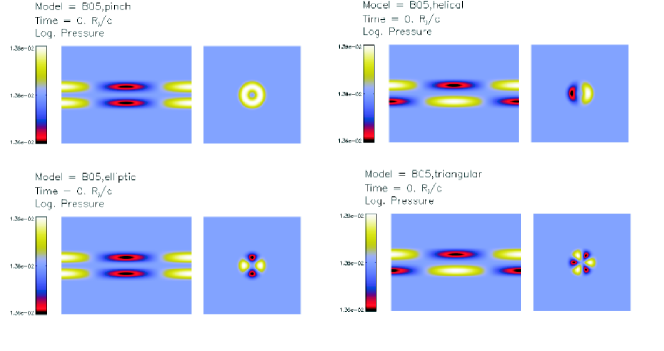
Figure 1: Structure of perturbations (axial and transversal cuts) in a generic 3D jet, as described by Eq. (5). Top left: pinching mode ($n=0$). Top right: helical mode ($n=1$). Bottom left: elliptical mode ($n=2$). Bottom right: triangular mode ($n=3$).

Frequencies of the excited modes, both helical and elliptical, are introduced in Eq. 5. These frequencies are computed from the observed wavelengths in LZ01, $\lambda^{obs}$, corrected for projection effects and relativistic motion of the wave (time delay), with velocity $v_{w}$($=0.23\,c$). We use $\omega=2\,\pi\,v_{w}/\lambda^{theor}$ (see Table 3), where

$$\lambda^{theor}=\frac{\lambda^{obs}(1-v_{w}/c\,\cos\theta_{j})}{\sin\theta_{j}},$$ (6)

where $\theta_{j}$ is the angle to the line of sight. We observe that, when computing the numerical solutions for the stability problem for the proposed jet parameters, the wavelengths and speeds obtained for the relevant modes (see Table 3) are different to those given in LZ01. This fact may be caused by errors in the angle to the line of sight or in the derived parameters in LZ01, including the wave speeds which are used in the transformation.

2.3.2 Results

To compare the results of the simulation with the numerical solution of the stability problem, we have solved the dispersion relation equation (e.g., Hardee har00 (2000)) for the parameters given in Table 2. Fig. 2 shows the solutions for the pinching, helical and elliptical surface, first and second body modes. Table 4 shows the characteristic wavelengths of the relevant modes.

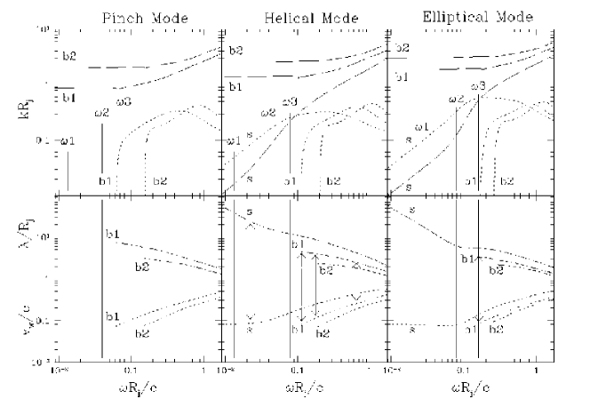
Figure 2: Solution of the stability problem for the parameters given in Table 2. In the upper plots, real (dashed lines) and imaginary (dotted lines) parts of the wavenumber are given as a function of frequency. In the lower plots, corresponding wavelengths and wave speeds are shown. Frequencies $\omega 1$, $\omega 2$ and $\omega 3$ correspond to those given in Table 3 for the simulation 3C273-A. Note that wavelengths for the elliptical modes in the plot are for a $180^{\circ}$ rotation of the ellipse and needs to be doubled for a complete rotation. This is because such a $180^{\circ}$ rotation generates a repetition of the structure in elliptical modes, therefore giving the impression of a complete wavelength. Arrows connecting the wavelength and wave speed plots indicate identified modes in the simulation 3C273-A (see text).

Table 4: Solutions of the stability problem in the fastest growing or resonant frequencies (indicated with an asterisk, column one lists the frequencies, column two the wavelengths and column three the wave speeds) and longest unstable wavelength (fourth column, $\lambda_{l}$)

Mode	$\omega^{*}$ ($c/R_{j}$)	$\lambda^{*}$ ($R_{j}$)	$v_{\omega}^{*}$ ($c$)	$\lambda_{l}$ ($R_{j}$)
Pinch b1	0.46	3.5	0.26	7.5
Pinch b2	0.86	1.8	0.25	3.1
Helical s	0.24	7.6	0.28	-
Helical b1	0.66	2.5	0.26	4.5
Helical b2	1.07	1.5	0.25	2.4
Elliptic s	0.19	5.3	0.16	-
Elliptic b1	0.85	1.9	0.26	3.2
Elliptic b2	1.27	1.3	0.25	2.0

Fig. 3 presents axial cuts made at two different times of the simulation. In Fig. 3 we observe a $\lambda\sim 20-25R_{j}$ helical structure in the upper plot that could be associated to $\omega_{2}$ (see Table 3). Fig. 4 shows several transversal cuts of the jet illustrating competition between the helical and elliptical modes. We can see how excited modes dominate at different positions and times in the jet. It is remarkable that elliptical structures show up close to the injection point, while helical modes, develop in the jet farther downstream. This agrees with the conclusions presented in LZ01. Nevertheless, we have not been able to clearly identify the elliptical mode in the longitudinal cuts. Fig. 5 shows longitudinal cuts of pressure perturbation (defined as the difference between the value of the pressure in a cell and the initial equilibrium pressure, $P-P_{0}$, with $P_{0}\sim 0.03\,\rho_{a}\,c^{2}$) at different jet radii, from which the dominant wavelengths could be identified in the simulated jet. We identify a $\lambda\sim 40-50\,R_{j}$ structure at $z<60\,R_{j}$ which we interpret as due to beating between two wavelengths of the first body helical mode at wavelengths $4.5\,R_{j}$ and $4\,R_{j}$, like that derived from the fits to the observations by LZ01, and given in Table 1 (3.9 and 4.1 mas). From plots of pressure perturbation at different radii (Fig. 5) we conclude that the radial structure of this beat can only be produced by the helical first body mode, as the fluctuations are stronger at $R_{j}/2$. The beating could also be produced by the elliptical surface mode, but the fact that pressure fluctuations are smaller at the jet surface rules out this possibility (see, e.g., Hardee har00 (2000)). At larger distance ($z>70R_{j}$) we have identified a large amplitude helical $\sim 25\,R_{j}$ wavelength and a shorter $2.5\,R_{j}$ wavelength superposed on the former one. In an axial cut of the pressure perturbation close to the axis we have identified an elliptical fluctuation with wavelength $\sim 3.5\,R_{j}$ at $z\sim 70-95\,R_{j}$ and a helical one with wavelength $2.5\,R_{j}$ at $z>100\,R_{j}$. All the modes that are reported in this paragraph are pointed in Fig. 2 with arrows indicating their wavelengths and wave speeds. We should keep in mind that the stability problem has been solved for the vortex sheet case and the jet in the simulations has a thick shear layer. This fact can introduce inaccuracies in the detection of modes in the simulation.

We have used all the identified structures in order to produce theoretical cuts of the pressure perturbation. Results are shown in Fig. 6. Note that here we have plotted $P/P_{0}$, whereas in Fig. 5 we plot $P-P_{0}$. The similarity to that obtained from the simulation is remarkable taking into account the fact that the presence of a shear layer, which may modify the stability problem solution (Perucho et al. pe+05 (2005)), has not been considered in the interpretation of the results.

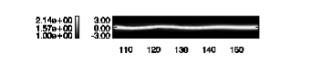
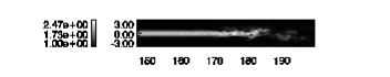
Figure 3: Map of Lorentz factor distribution of a portion of the jet at a time before disruption, where a large amplitude wave is apparent (top panel, $t=320\,R_{j}/c$) and at the last frame (bottom panel, $t=1097\,R_{j}/c$). Coordinates are in jet radii. The vertical scale size is increased by a factor of 4 to better represent the jet structure.

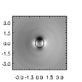
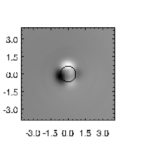
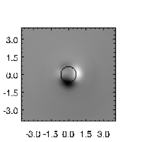
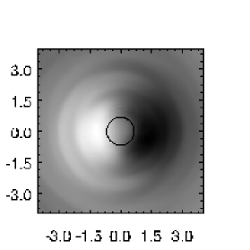
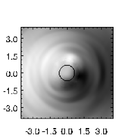
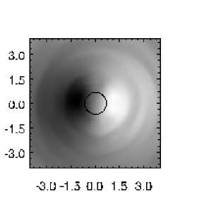
Figure 4: Transversal structure of pressure perturbations (lighter shading indicates higher pressure values). Solid line indicates $v_{z}=0.8\,c$ contour. Three left panels: Cuts at $35\,R_{j}$, for $t=70,\,140,\,200\,R_{j}/c$ where the elliptical or double helical mode rotation is apparent. Three right panels: Cuts at $105\,R_{j}$, for $t=210,\,220,\,240\,R_{j}/c$ where the helical mode rotation is apparent.

Figure 5: Longitudinal cuts of pressure perturbation at different radii ($R_{j}/8$ top left, $3R_{j}/8$ top right, $5R_{j}/8$ bottom left, $7R_{j}/8$ bottom right) and in symmetric positions with respect to the jet axis at $t=250\,R_{j}/c$.

Figure 6: Theoretical computation of the pressure perturbation produced by the combination of modes identified in the simulation, compared to Fig. 5. Lines indicate cuts at different distances from the axis. Dotted line stands for pressure perturbation at $R_{j}/8$, dashed line at $3R_{j}/8$, dash-dot line at $5R_{j}/8$, and long dashed line for $7R_{j}/8$. The wavelengths and wave speeds of the modes applied in this plot are indicated with arrows in Fig. 2. These are the helical first body mode at $\lambda=4.53\,R_{j}$, $\lambda=4.04\,R_{j}$ for $z<60\,R_{j}$, the helical surface mode at $\lambda=24.3\,R_{j}$ and first body mode at $\lambda=2.47\,R_{j}$ and the elliptical first body mode at $\lambda=3.22\,R_{j}$ for $z>70\,R_{j}$. We have used a linearly growing amplitude between $z=70\,R_{j}$ and $z=120\,R_{j}$ for the helical surface mode, between $z=70\,R_{j}$ and $z=105\,R_{j}$ for the helical first body mode, and constant amplitude from those distances. We have also used constant amplitude at $z<70\,R_{j}$ for the elliptical body mode.

When comparing the results given in the previous paragraphs with those from LZ01, we find differences in the typical wave speeds for the modes observed in the simulation ($\sim 0.1c$), obtained from the solution to the stability problem (Fig. 2), compared to those given in LZ01 from the linear approximations ($0.23c$). This could be caused by the uncertainties of the linear approximations, Eqs. (1) and (2.1), used in LZ01. In deriving approximations, a large classical Mach number is assumed ($M_{j}=v_{j}/c_{s,j}\gg 1$), but this is not generally the case for hot jets, for which $c_{s,j}\simeq 0.57$, and thus, $M_{j}\leq 1.75$. To investigate the uncertainties introduced by this fact, we have used numerical solutions of the dispersion relation for different cases and compared them with the results of the approximations. Results show that the errors in the determination of characteristic wavelengths with linear approximations can reach a factor two for small Mach numbers, while for $M_{j}>5$, the errors are smaller than $30\%$. This could result in significant errors with the identification of the modes. Another difference we find comes from the fact that we do not observe the elliptical surface mode in the simulation, although it is fitted from observations in LZ01 and we find in the solution to the stability problem that it has a short growth length (Fig. 2). This could be due to the radial structure of the initial perturbation ($\propto\sin(\pi r)/\cosh(r)$) giving zero initial amplitudes at the jet surfaces, and therefore suppressing the surface modes. Otherwise we would expect the elliptical surface mode to dominate at $z<60\,R_{j}$ and maybe also farther downstream, as seen in the growth rates shown. Somehow, however, the helical surface mode seems to develop at distances $z>70\,R_{j}$, and we think that this may be due to slight changes in the radial structure of the perturbations with downstream evolution as they grow in amplitude and modes interact among them.

In the frame of the comparison between results from the simulation and linear analysis and from the fits in LZ01, we now focus our discussion on the three main structures observed in the simulation. We define $\lambda^{sim}_{1}=4\,R_{j}$, $\lambda^{sim}_{2}=25\,R_{j}$ and $\lambda^{sim}_{3}=50\,R_{j}$ as the characteristic wavelengths in the simulation. Propagation speeds of the perturbations can be measured in the section of the jet dominated by the linear growth of instability. Although this is difficult due to the sparsity of the data frames, we derive the wave speed of the disruptive mode ($\lambda^{sim}_{2}$) following the motion of the large amplitude wave (see Fig. 3) from frame to frame, which gives $v_{w,2}\simeq 0.38\,\rm{c}$, or any fraction of this number. From Fig. 2 we can tell that the mode must be moving at $v_{w}\sim 0.09c$. Another wave speed of the system is obtained from the rotation of the elliptical patterns similar to those shown in Fig. 4, which yields $v_{w}\simeq 0.2\,\rm{c}$. Unfortunately, we have not been able to find the wavelength of this elliptical mode in the pressure perturbation plots. We note that this speed is close to the value of $v_{w}$ given in LZ01 and it is different from the one predicted by the solution of the stability problem (Fig. 2) for the helical first body modes that we claimed to generate this long scale structure as a beating pattern. This can be due to the presence of a thick shear layer that certainly changes the picture of the solution to the stability problem. It could also be due to the structure that we have used to measure the speed having been artificially generated by the interaction of helical modes in $180^{\circ}$ phase, and therefore giving a different velocity to those of single modes. Also, we use, as a limit for small wavelength perturbations, a wave speed equal to that of the flow ($v_{w,1}\simeq 0.88\,c$).

The parameters of the simulated and resulting observed structures are given in Table 5. To reconcile the simulations with the observational results we calculate $\lambda^{obs}$ from $\lambda^{sim}$ ($\lambda^{theor}$ in Eq. 6), using the three different values of $v_{w}$ mentioned in the previous paragraph. It should be noted that the two longest modes identified in the simulation have an observational counterpart when we take $v_{w}=0.09c$, which is a value close to that given by the stability problem for most of the identified modes in the simulation (see Fig. 2). The $\lambda^{sim}_{2}$ mode could be identified with the fitted helical second body mode with the wavelength of 2 mas in LZ01. The $\lambda^{sim}_{3}$ mode could correspond to the fitted first body modes at the wavelength of 4 mas in LZ01. However, $\lambda^{sim}_{2}$ is identified as a helical surface mode, thus not coincident with the fitted second body mode to the 2 mas structure and we have used the long envelope of the beating structure in order to derive a 4 mas structure, which is interpreted as two helical body modes with a similar wavelength in LZ01. Using the given wave speed of $v_{w}=0.09c$, the term $\sin\theta_{j}$ has larger influence on the result than the term $1-v_{w}\cos\theta_{j}$ in Eq. 6, so only larger angles to the line of sight would give larger $\lambda^{obs}$ from a given $\lambda^{sim}$: the $4\,R_{j}$ wavelength would result in a 1 mas observed structure at $45^{\circ}$ and the $25\,R_{j}$ wavelength would result in a 6 mas observed structure at the same angle to the line of sight. Nevertheless, this angles are ruled out by jet to counter-jet (still not observed) flux ratios and by recent observations by Jorstad et al. (jor+05 (2005)). At that wave speed, shorter angles to the line of sight would result in even shorter observed wavelengths. This translates into the need of larger wavelengths in the simulation in order to fit them to observations, but Fig. 2 tells us that we are in the longest unstable wavelength limit for body modes, so this seems unrealistic.

Why we do not see the 12 mas elliptical surface mode is thought to be due to the radial structure of the initial perturbation ($\propto\sin(\pi r)/\cosh(r)$) which, as stated above, gives zero initial amplitudes at the jet surfaces, therefore suppressing these modes. Moreover, the 12 mas mode, with the wave speed given in LZ01, would require a $110\,R_{j}$ wavelength in the simulation, which is difficult to observe even in a grid as large as was used here, in particular when shorter harmonics grow fast and disrupt the flow.

Table 5: First column give identified wavelengths in LZ01 from shorter to longer, in the second column we have written characteristic wavelengths in the simulation also in increasing order, and the last three columns give the wavelengths as observed depending on the wave speed.

$\lambda^{obs}\,[\rm{mas}]$	$\lambda^{sim}\,[R_{j}]$	$\lambda^{sim}_{v_{w}=0.09\,c}\,[\rm{mas}]$	$\lambda^{sim}_{v_{w}=0.23\,c}\,[\rm{mas}]$	$\lambda^{sim}_{v_{w}=0.88\,c}\,[\rm{mas}]$
2	4	0.36	0.44	2.27
4	25	2.28	2.7	14.3
12	50	4.56	5.5	28.5

2.3.3 Nonlinear regime

Nonlinear effects become important at time $t=350\,R_{j}/c$ with the disruption of the head of the jet due to the longest helical mode $\lambda^{sim}_{2}\simeq 25\,R_{j}$. After that point perturbations produced at the disruption point propagate backwards slowly as a backflow. The disruption point itself moves downstream due to constant injection of momentum at the inlet and the change of conditions around the jet. The disruption point advances from $160\,R_{j}$ to $180\,R_{j}$ by the end of the simulation (see Fig. 3).

Morphology of the jet at the end of the run (lower panel of Fig. 3) is thus different from the observed source mainly due to the disruption of the jet. These difference may result from the development of a disruptive mode in the simulation which is not present in the real jet due to, for example, magnetic fields or an opening angle in the jet, not taken into account here. Uncertainties in the calculation of the physical parameters from the characteristic wavelengths following Eqs. (1) and (2.1), as discussed in previous paragraphs, can be a source of error in the determination of the parameters of the jet, which, in turn, influence the long term stability properties.

Disruption of the jet in the simulation contradicts apparently the fact that the jet is observed on much larger scales. It should be noted however that the disruption point still propagates outward at $v\sim 0.03\,c$, at the end of the simulations. This implies that the simulation has not run long enough to reach a quasi-steady stage. It is also possible that the disruption observed is a transitory phase and that the simulation should have run longer in order to allow the jet to move downstream. If a stabilizing factor is needed in order to explain the jet in 3C273, we suggest several possibilities: 1) a thicker shear layer (Birkinshaw bir91 (1991), Hardee & Hugues hah03 (2003), Perucho et al. pe+06 (2006)), 2)  inclusion of the superluminal components in the simulations, as faster jets are much more stable against K-H instability (see Perucho et al. 2004b , Perucho et al. pe+05 (2005)), 3) a decreasing density atmosphere (Hardee har82 (1982, 1987), Hardee et al. har05 (2005), where it is shown, in the case of the jet in 3C 120, that the expansion of the jet provides a stabilizing influence), which must be the case as can be derived from the outward dimming due to adiabatic expansion of the observed jet in the parsec scale , 4) a stabilizing configuration of magnetic field (Rosen et al. ro+99 (1999), Frank et al. fra+96 (1996), Jones et al. jon+97 (1997), Ryu et al. ryu+00 (2000), Asada et al. asa+02 (2002)). The cumulative effect of these factors would effectively make the jet more stable already on the time scales probed by the simulation.

2.4 Simulation 3C273-B

2.4.1 Initial setup

In this simulation, the stationary flow is perturbed by precession and periodical ejections of faster components. The initial conditions are similar to those in the first simulation. The width of the shear layer is $\sim 0.6\,R_{j}$ ($m=8$). The precession frequency is derived from the observed $\sim 15$ yr ($6\,R_{j}/c$ in the code units) periodicity of position angle variations (Abraham et al. abr+96 (1996)). The frequency of ejections of components is set by the reported $\sim 1$ yr ($0.4\,R_{j}/c$) periodicity in the optical light curve (Babadzhanyants and Belokon bb93 (1993)). The duration of each ejection is estimated to be $\sim 2$ months ($0.066\,R_{j}/c$), set by the approximate inspiralling time from an orbit at $\approx 6R_{\mathrm{G}}$ around a $5.5\times 10^{8}\mathrm{M}_{\odot}$ black hole. The amplitude of the precession is set by the true opening angle ($0.4^{o}$) of the jet obtained by deprojecting the apparent opening of $1.5^{o}$. This precession is included in transversal velocities at the injection point as follows:

$$\overrightarrow{v_{\perp}}=A_{0}v_{z}(\cos(\omega t),\sin(\omega t))$$ (7)

where $\overrightarrow{v_{\perp}}$ and $v_{z}$ are the transversal and axial components of the velocity, $t$ is time, $A_{0}=6.83\,10^{-3}$ is the initial amplitude, and $\omega\sim 1.01\,c/R_{j}$ is the angular frequency calculated from the precession period of $\sim 15\,\rm{yrs}$.

The fluid in the injected components is considered to have the same density as the underlying flow and to be in pressure equilibrium with it. Velocity of the fluid in components is taken as constant, with the mean value of Lorentz factor $\gamma_{\mathrm{c}}\simeq 5$ as reported in Abraham et al. (abr+96 (1996)). The components are generated as shells of fluid with a diameter of $0.5\,R_{j}$ ejected along the axis.

The numerical grid for this simulation covers $30\,R_{j}$ (axial) times $6\,R_{j}$ times $6\,R_{j}$ (transversal), i.e., $24\,\rm{pc}\times 4.8\,\rm{pc}\times 4.8\,\rm{pc}$. The axial dimension of the grid is related to the ejection of the components. We take into account that the wavelength induced by the precession of components, if they move ballistically, is $\lambda_{\mathrm{c}}\sim P\,v_{\mathrm{c}}$, where $P$ is the precession period and $v_{\mathrm{c}}$ is the injection velocity of the fluid in the components. This gives $\lambda_{\mathrm{c}}\sim 6\,R_{j}$, and we have chosen the grid of $5\,\lambda_{\mathrm{c}}$ to allow the wave to become apparent.

The resolution of the grid is 16 cells$/R_{j}$ in the transversal direction and 32 cells$/R_{j}$ in the direction of the flow. An extended grid is introduced in both transversal and axial directions. In the radial directions, it has 36 cells reaching out to $15\,R_{j}$ on each side of the jet (increasing the cell size by $7.7\%$ from one cell to the next). In the axial direction the extended grid has 192 cells, reaching up to $45\,R_{j}$. This simulation has lasted for a time of $70\,R_{j}/c$ (i.e., more than two light crossing times of the grid).

2.4.2 Results

Fig. 7 shows the solutions of the linear stability problem for the jet parameters given in Table 2 and indicates the characteristic wavelengths arising un this simulation. Fig. 8 shows longitudinal cuts of pressure perturbation at different jet radii at time $40\,R_{j}/c$. Inspection of the longitudinal cuts indicates that, close to the injection point and to the jet axis, a symmetric, short wavelength perturbation generated by the fast components dominates the structure of the flow. Its wavelength is $\lambda^{sim}_{1}=0.4\,R_{j}$, and it is clearly related to the ejection period of components ($0.4\,R_{j}/c$). After $3-4\,R_{j}$, the presence of the fast components is also evident in the jet boundary (at $r=7/8R_{j}$). These high-frequency and short-wavelength structures are damped at $z>10\,R_{j}$, as expected to occur for perturbations with wavelengths smaller than the shear layer width. Close to the jet boundary, the most pronounced structure is the typical antisymmetric pattern of helical motion induced by the precession ($\lambda^{sim}_{2}\sim 3.7\,R_{j}$). This structure is driven by the precession of the injected components and it couples to the helical surface mode at a frequency of $0.8\,c/R_{j}$. A pinch mode structure with a wavelength $\lambda^{sim}_{2}=3.7\,R_{j}$ is also observed at $r=R_{j}/8$, coinciding with the maximum growth of the first body mode (see Fig. 7 and Table 4).

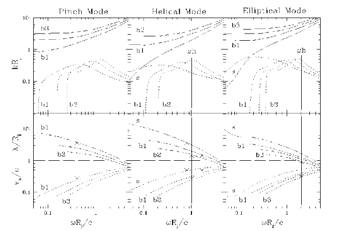
Figure 7: Solution of the stability problem for the parameters given in Table 2 with the characteristic frequencies for simulation 3C273-B. Frequency $\omega_{h}=1.01c/R_{j}$ corresponds to that excited in the simulation 3C273-B. Arrows connecting the wavelength and wave speed plots indicate identified modes in the simulation 3C273-B (see text).

Farther downstream and close to the jet center, there is a $\lambda^{sim}_{3}=0.9\,R_{j}$ wavelength on top of the longer pinch mode ($\lambda^{sim}_{2}$). This short wavelength coincides with the maximum growth rate of the elliptical third body mode at the helical driving frequency ($1.01\,c/R_{j}$) (see Fig. 7 and Table 4). We remind the reader that this is frequency correspond to a 360^∘ turn, as explained in the caption of Fig. 2. The radial structure of this mode in the simulation is also coincident with the theoretical structure of the third body elliptical mode, with the maximum amplitude at $r=R_{j}/4$ and decreasing amplitude at larger radii. The helical driving frequency falls very close to the maximum growth of the second body helical mode with wavelength $\lambda^{sim}_{4}=1.5\,R_{j}$, observed in Fig. 8. However, the radial structure found in the simulation is somehow a mixture of the second body mode with that of the first body mode. We expect the second body mode to have an amplitude maximum at $r=1/8R_{j}$, but we find that this maximum occurs at $r=3/8R_{j}$. The first body mode at this wavelength develops an amplitude maximum at $r=3/8R_{j}$, which is coincident with the one found in the simulation, although the amplitude at $r=1/8R_{j}$ found in the simulation is too large for this mode. We interpret this as the second body mode being triggered at the driving frequency, which in turn excites the first body mode at the same wavelength. Both modes seem to be triggered out of phase and interfere destructively in the inner jet, but the first body mode dominates in the mid jet region and both decline in amplitude towards the jet surface. Comparison of smaller and larger radius plots of pressure perturbation in Fig. 8 shows large positive offsets observed at larger radii. This indicates possible drifting of components (shocks) to outer radii of the jet as they follow the helical path given by the surface mode (similar to what has been reported by LZ01). This feature would produce enhanced emission regions at the positions of the helix in which the flow moves in a direction closer to the line of sight. Using all of the modes identified in the simulation we have computed a theoretical representation of the pressure perturbation in the jet. Fig. 9 shows the resulting axial cuts of the pressure perturbation and indicates that the theoretical calculation generates most of the structures found in the simulation, except those which are intrinsically nonlinear (for instance, the injected components at the jet inlet and those structures at outer jet radii farther downstream).

Figure 8: Longitudinal cuts of pressure perturbation at different radii ($R_{j}/8$ top left, $3R_{j}/8$ top right, $5R_{j}/8$ bottom left, $7R_{j}/8$ bottom right) and in symmetric positions with respect to the jet axis at $t=40\,R_{j}/c$. Short wavelength ($\lambda^{sim}_{1}=0.4\,R_{j}$ and $\lambda^{sim}_{3}=0.9\,R_{j}$) structures are observed close to the jet axis. The amplitude of the first structures decrease downstream as a consequence of the drift of components to outer radial positions due to the precessional motion and their interaction with the underlying flow. Also at positions close to the axis, we find a structure with wavelength $\lambda^{sim}_{3}=1.5\,R_{j}$. Short wavelength symmetric ($\lambda^{sim}_{1}=0.4\,R_{j}$) and longer wavelength antisymmetric ($\lambda^{sim}_{2}=4\,R_{j}$) structures are also observed at outer radial positions. The longer structure dominates close to the injection, before the components expand and/or drift from the axis to the jet boundaries, when short scale structures can be observed to be modulated by the longer one (from $z\sim 4\,R_{j}$). After this, at $z=9\,R_{j}$, the antisymmetric longer structure grows in amplitude, with some spikes that can be associated with the drift of the components due to their precessional motion.

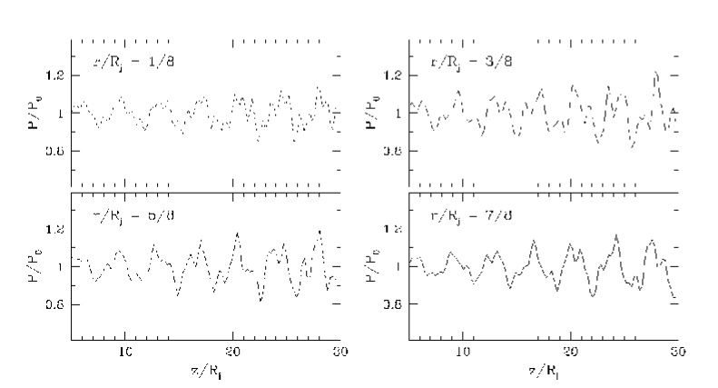
Figure 9: Theoretical computation of the pressure perturbations produced by the combination of modes identified in the simulation. Different panels indicate cuts at different distances from the axis in the X-Z plane. The wavelengths and wave speeds of the modes contributing to this perturbations are marked by arrows in Fig. 7. These are the first pinch body mode at $\lambda=3.7\,R_{j}$, the helical surface mode at $\lambda=3.7\,R_{j}$, helical first and second body modes at $\lambda=1.5\,R_{j}$, and the elliptical third body mode at $\lambda=0.9\,R_{j}$. We have used a linearly growing amplitude for the modes. This perturbations can be compared with the structures identified in Fig. 8. Main differences between this plot and Fig. 8 are due to nonlinearities introduced by injected components, mainly close to the injection on the jet axis and at outer radii farther downstream.

The complexity of the structure is further illustrated by the surface plot of the flow Lorentz factor shown in Fig. 10. Although in this figure we only see patterns in the fluid, comparison of the wavelengths seen here and in Fig. 8 allows us to identify the wavelengths derived from the fluid patterns in Fig. 10 and from the frequency of injection of components. The middle panel of Fig. 10 (Lorentz factor $\gamma=2.5$) indicates that the periodicity induced by individual jet components dominates the structure up to distances $z\sim 10-15\,R_{j}$, but farther downstream the components expand longitudinally and start to interact with each other, generating a semi-continuous structure that is dominated by the helical motion induced by the precession. The top panle of Fig. 10 (Lorentz factor $\gamma=3.0$) indicates that the distinct regions of the flow moving at higher speed disappear downstream. This can be explained by the deceleration of the fluid in the components. The deceleration can be caused either by the interaction with the background flow, or by a radial and longitudinal expansion. These results are in agreement with results by Lobanov and Zensus (lz99 (1999)), and Lobanov and Roland (lr01 (2001)), suggesting that shocks dominate the jet structure close to the nucleus, and that fluid instabilities become important farther downstream. On the other hand, it is not clear at the moment whether stronger fluid components (i.e., faster and denser) could survive longer in the jet. We finally note that the precession wavelength obtained from the simulations is smaller than the one calculated theoretically from the advance speed of components ($\lambda^{sim}_{2}=4\,R_{j}$ versus $\lambda_{c}\sim 6\,R_{j}$), which maybe taken as an indication of non-ballistic motion of the components.

Table 6: First column gives the observed wavelengths in the simulation, and the last three columns give this wavelengths as observed depending on the wave speed. We have used, for the wave speed, some of those obtained from Fig. 7 for the identified modes (second to fourth columns), the underlying flow speed (fifth column) and the maximum speed from the components (sixth column).

$\lambda^{sim}$ [$R_{j}$]	$\lambda^{obs}_{v_{w}=0.25\,c}$[mas]	$\lambda^{obs}_{v_{w}=0.4\,c}$[mas]	$\lambda^{obs}_{v_{w}=0.5\,c}$[mas]	$\lambda^{obs}_{v_{w}=0.88\,c}$[mas]	$\lambda^{obs}_{v_{w}=0.94\,c}$[mas]
0.4	0.045	0.05	0.07	0.23	0.37
0.9	0.1	0.12	0.15	0.51	0.83
1.5	0.17	0.2	0.25	0.85	1.4
4	0.45	0.53	0.67	2.27	3.7

In Table 6 we list possible observed wavelengths corresponding to the two main wavelengths identified from the simulation. It is clear that the observed wavelength of precession ($18\,\rm{mas}$) cannot be recovered even with extremely fast components ($v_{w}=c$ gives $\lambda^{obs}=10mas$) with the adopted viewing angle of $15^{\circ}$. Moreover, if we consider the mean apparent proper motion of $0.93\,h^{-1}\rm{mas/yr}$ (Abraham et al. abr+96 (1996)), the apparent speed is $\beta_{app}\sim 10$. This speed cannot be reconciled with a viewing angle of $15^{\circ}$, as the resulting intrinsic speed is larger than 1, and it would require a Lorentz factor of $\gamma=10$ if the viewing angle is reduced to $10^{\circ}$. Recent work by Jorstad et al. (jor+05 (2005)) indicates that the jet in 3C273 can have a viewing angle as small as $6^{\circ}$ and component Lorentz factors of $\gamma\sim 10.6$. These numbers would transform $\lambda^{sim}_{2}=4\,R_{j}$ into an observed wavelength $14.1\,\rm{mas}$. This wavelength is in fair agreement with the $18\,\rm{mas}$ mode assigned to precession in LZ01. In summary, either the precession period should be longer, or the viewing angle should be smaller than $15^{\circ}$ and component Lorentz factors higher than $\gamma=3$, in order to reconcile the 18 mas structure with precession.

Figure 10: Surface plots for three different values of Lorentz factor: Upper panel, $\gamma=3.0$; middle panel, $\gamma=2.5$; lower panel, $\gamma=2.0$. The precession motion, coupled to a helical mode, is more apparent on the slower, underlying flow, moving at $\gamma=2.0-2.5$, as shown in LZ01. The surface plot for $\gamma=3.0$ illustrates the appearance of the jet at higher frequencies and smaller viewing angles, where the emission is dominated by a more relativistic plasma.

Another question addressed by this simulation is whether the periodic injection of fast components could generate smaller structures observed by LZ01 (the $2\,\rm{mas}$ and $4\,\rm{mas}$ modes), where these wavelengths are identified with the elliptical modes of Kelvin-Helmholtz instability. In our simulation, the fast components generate mainly pinching modes, although this is simply due to their symmetric nature. Again, we find that the structures generated in the simulation are small compared to those observed. However, in the simulation, the fluid in the components moves with a smaller speed than the injection one ($\gamma=5$, see Fig. 10) and therefore, smaller than that found from the observations ($\gamma\sim 5-10$). We relate this fact to the possible slowing of the components themselves as they propagate downstream. As pointed out before, a possible cause for this could be that the simulated fluid injected in components has the same density as the background flow, whereas if it was denser (as could be expected as generated from strong accretion activity) or propagating in a decreasing density atmosphere, this fluid would have larger inertia and would generate faster components. We find that, in order to produce a 4 mas structure, we need the Lorentz factor of components to be $\gamma\sim 30$, whereas $\gamma\sim 15$ is required to explain the 2 mas wavelength, if we keep the 1 yr period. Adopting the longest measured period of the ejections of 1.7 yrs (Abraham and Romero ar99 (1999)), these values would be reduced to $\gamma\sim 17$ and $\gamma\sim 8.5$, respectively. The same authors gave a periodicity in the injection Lorentz factor of about 4 yrs; if we consider this period as the generator of short modes, $\gamma\sim 7.5$ and $\gamma\sim 4$ could explain those structures. The latter values agree well with the Lorentz factors inferred from the observed kinematics of the jet. This means that the 2 and 4 mas wavelengths should be associated only with the strongest and fastest ejections occurring roughly once every 4 yrs. With the jet parameters given by Jorstad et al. (jor+05 (2005)), the inferred wavelength for the shortest symmetric structure ($0.4\,R_{j}$) is $1.4\,\rm{mas}$, which is within a factor of 3 from the 4 mas wavelength identified in LZ01 with the elliptical first body mode. The symmetric or pinching nature of the perturbations induced by such components could not explain the double helix structure in the jet, but we observe in the simulation that elliptical modes can be triggered by the presence of pinching and helical perturbations.

3 Conclusions

We have performed two numerical RHD simulations with different initial setups in order to study the physical processes generating the observed structures in the parsec-scale radio jet in the quasar 3C 273. In the simulation 3C273-A, we have included a general set of helical and elliptical perturbations in a long jet with the basic physical parameters adopted from LZ01. In the simulation 3C273-B, we have used a shorter jet with the same physical parameters and have included precession and injection of fast components. The simulation 3C273-A was aimed to generate structures with wavelengths similar to those measured by LZ01 from the growth of Kelvin-Helmholtz perturbations. The simulation 3C273-B was designed to check if by combining the ejection of superluminal components and jet precession, with the periodicities reported in Babadzhanyants and Belokon (bb93 (1993)) and Abraham et al. (abr+96 (1996)), the same structures could be generated.

We find that the structures generated in simulation 3C273-A are of the same order in size as those observed, if the relativistic propagation effects of the waves are taken into account. We observe in the solution of the stability problem that the instability modes found in the simulation propagate at mildly relativistic speeds. These wave speeds differ from those derived from the approximations used in LZ01. This can be due to the uncertainties introduced by the approximations to the characteristic wavelengths in the interpretation of the observations in LZ01. However, we show that wavelengths similar to the observed ones are found for the wave speed given by the solution of the linear problem, although the modes fitted in LZ01 and those used here for the same wavelengths are not coincident. The solutions of the stability problem applied to the adopted wave speeds (0.23 $c$) and line of sight ($15^{\circ}$) show that any body modes present in the jet should be much shorter than those fitted in LZ01. It should be noted that these differences do not rule out the presence of Kelvin-Helmholtz instability in parsec-scale jets. Despite difficulties in the mode identifications, the structures generated in the simulation are similar to those observed by LZ01.

Regarding the long-term stability of the flow, we note that the jet in the simulation 3C273-A is disrupted at $\sim 170\,\rm{pc}$ from the inlet, contrary to the observations tracing the jet in 3C273 up to $60\,\rm{kpc}$ away from the source. The reasons for this difference may be found in the conjunction of several factors. 1) The numerical simulation does not run long enough to reach a fully steady-state regime. The disruption point moves downstream along the simulation, which could imply that the disruption is a transitory phase. 2) Magnetic fields have not been taken into account neither in the linear analysis, nor in the numerical simulation - and it should be noted that the magnetic fields may be dynamically important at parsec scales (Rosen et al. ro+99 (1999), Frank et al. fra+96 (1996), Jones et al. jon+97 (1997), Ryu et al. ryu+00 (2000), Asada et al. asa+02 (2002)). 3) We only simulate the underlying flow, without considering the faster and possibly denser fluid in the superluminal components. 4) Inaccuracies in the linear analysis approximations can lead to large uncertainties in physical parameters derived. 5) Differential rotation of the jet, shear layer thickness (Birkinshaw bir91 (1991), Hardee & Hugues hah03 (2003), Perucho et al. pe+06 (2006)), and a decreasing density external medium could also play an important role (implying jet expansion; see Hardee har82 (1982, 1987), and Hardee et al. har05 (2005)). 6) Arbitrary initial amplitudes of perturbations were chosen for the simulation, so we could have included too large perturbations. A combination of these factors could well change the picture of the evolution of the jet in terms of its stability properties. The effects of the rotation and magnetic fields on the stability of jets remain unclear, since no systematic numerical study has been performed up to now.

In the simulation 3C273-B, we studied the effect of precession on the jet evolution and investigated the possibility that the short wavelength structures found in LZ01 were not due to K-H instabilities but due to the periodicities induced in the flow by the ejection of components. We demonstrate that such non-linear features as superluminal components generate linear structures in the form of Kelvin-Helmholtz instabilities which can be analyzed in the framework of linear perturbation analysis. One of the main conclusions that can be derived from this simulation is that helical twists can be excited by periodic injections if there is some induced helicity in the system. This helicity is induced in our simulation by the helical perturbation frequency, but in real jets this helicity could be induced by helical jet magnetic fields and/or by jet rotation. We have also shown that, in order to explain the observed $18\,\rm{mas}$ wavelength in terms of precession, either longer driving periodicities than the $15\,\rm{yr}$ suggested by Abraham & Romero (ar99 (1999)) would be needed, or this wavelength must be induced by very fast components observed in a jet moving at a viewing angle $\theta<15^{\circ}$. The fast components could only generate the shorter wavelengths given in LZ01 ($\lambda=2$ mas and $\lambda=4$ mas) if a proper combination of the velocities and injection periodicities is used. Altogether, we find that inclusion of faster components and precession with the $15\,\rm{yr}$ periodicity does not explain well the observed wavelengths and periodicities. This gives more weight to the general conclusion about K-H instability acting prominently in the flow.

In the future, numerical simulations of this kind may be used to constrain the basic parameters of the flow such as the viewing angle and the component speed. Inclusion of magnetic fields, differential rotation and the effects of an atmosphere with a decreasing density could help reconciling better the simulations with the observed structures. In this way, for example, an increase of the jet radius due to decreasing external density could cause a downstream increase of wavelengths of K-H instability modes (Hardee et al. har05 (2005)). This remains to be seen with future, full-fledged RMHD simulations of the relativistic jet in 3C 273. The scope of the present work could be expanded to other sources, and applied to prominent jets for which the transversal structure may be resolved, such as 3C 120, extending the work done by Hardee et al. (har05 (2005)) by performing numerical simulations.

- (1) Abraham, Z., Carrara, E. A., Zensus, J. A., Unwin, S. C. 1996, A&AS, 115, 543.
- (2) Abraham, Z., Romero, G. E. 1999, A&A, 344, 61.
- (3) Aloy, M.A., Ibáñez, J.M, Martí, J.M, and Müller, E. 1999, ApJSS, 122, 151
- (4) Asada, K., Inoue, M., Uchida, Y., et al. 2002, PASJ, 54, L39.
- (5) Babadzhanyants, M. K., Belokon’, E. T. 1993, Astron. Zh., 70, 241.
- (6) Begelman, M. C., Blandford, R. D., Rees, M. J. 1984, Rev. Mod. Phys., 56, 255.
- (7) Belokon’, E. T. 1981, Astron. Zh., 68, 1.
- (8) Birkinshaw, M. 1991, MNRAS, 252, 505.
- (9) Conway, R. G., Davis, R. J., Foley, A. R., Ray, T. P. 1981, Nature, 294, 540.
- (10) Conway, R. G., Garrington, S. T., Perley, R., Biretta, J. A. 1993, A&A, 267, 347.
- (11) Courvoisier, T. J.-L. 1998, A&ARv, 9, 1.
- (12) Davis, R. J., Unwin, S. C., Muxlow, T. W. B. 1991, Nature 354, 374.
- (13) Frank, A., Jones, T.W., Ryu, D., & Gaalaas, J.B. 1996, ApJ, 460, 777.
- (14) Gómez, J. L., Alberdi, A., Marcaide, J. M. 1993, A&A, 274, 55.
- (15) Gómez, J. L., Alberdi, A., Marcaide, J. M. 1994, A&A, 284, 51.
- (16) Gómez, J. L., Alberdi, A., Marcaide, J. M., Marscher, A. P., Travis, J. P. 1994, A&A, 292, 33.
- (17) Hardee, P. E. 1982, ApJ, 287, 523.
- (18) Hardee, P. E. 1984, ApJ, 303, 111.
- (19) Hardee, P. E. 1987, ApJ, 313, 607.
- (20) Hardee, P. E. 2000, ApJ, 533, 176.
- (21) Hardee, P. E. 2003, ApJ, 597, 798.
- (22) Hardee, P. E., Clarke, D. A., Rosen, A. 1997, ApJ, 485, 533.
- (23) Hardee & Hughes 2003, ApJ, 583, 116.
- (24) Hardee, P.E., Walker, R.C., Gómez, J.L. 2005, ApJ, 620, 646
- (25) Hazard, C. Mackey, M.-B., Shimmins, A.J. 1963, Nature, 197, 1037.
- (26) Hutchings, J. B., Stoesz, J., Veran, J.-P., Rigaut, F. 2004, PASP, 116, 154.
- (27) Jester, S. 2001, Ph.D. Thesis, U. Heidelberg.
- (28) Jester, S., Röser, H.-J., Meisenheimer, K., Perley, R., Conway, R. G. 2001, A&A, 373, 447.
- (29) Jones, T.W., Gaalaas, J.B., Ryu, D., & Frank, A. 1997, ApJ, 482, 230.
- (30) Jorstad, S.G., Marscher, A.P., Lister, M.L., Stirling, A.M., Cawthorne, T.V., Gear, W.K., Gómez, J.L., Stevens, J.A., Smith, P.S., Forster, J.R., Gabuzda, D.C., Robson, E.I. 2005, submitted to AJ
- (31) Kaspi, S., Smith, P. S., Netzer, H., et al. 2000, ApJ, 533, 631
- (32) Krichbaum, T. P. Witzel, A., Zensus, J. A. 2000, in Proc. of the 5th EVN Symposium, eds. J. E. Conway, A. J. Polatidis, R. S. Booth, Y. W. Pihlström (Onsala Space Observatory: Onsala), 25.
- (33) Lobanov, A. P. 1998, A&AS, 132, 261.
- (34) Lobanov, A. P., Zensus, J. A. 1999, ApJ, 521, 509.
- LZ (01) Lobanov, A. P., Zensus, J. A. 2001, Science, 294, 128 (LZ01).
- (36) Lobanov, A. P., Roland, J. 2001, in ASP Conference Proceedings v. 250, “Particles and Fields in Radio Galaxies”, eds. R. A. Laing, K. M. Blundell (ASP: San Francisco), 195.
- (37) Lobanov, A. P., Carrara, E., Zensus, J. A. 1997, Vistas in Astronomy, 41, 253.
- (38) Lobanov, A. P., Zensus, J. A., Abraham, Z., et al. 2000, Advances in Space Research, 26, 669.
- (39) Lobanov, A. P., Hardee, P. E., Eilek, J. A. 2003, NewAR, 47, 629.
- (40) Marshall, H. L., Harris, D. E., Grimes, J. P., et al. 2001, ApJ, 549, L167.
- (41) Marscher, A. P. 1980, ApJ, 235, 386.
- (42) Marscher, A. P., Gear, W. K. 1985, ApJ, 298, 114.
- (43) Martí, J.M, Müller, E., Font, J.A., Ibáñez, J.M, and Marquina, A. 1997, ApJ, 479, 151
- (44) Neumann, M., Meisenheimer, K., Röser, H.-J. 1997, A&A, 326, 69.
- (45) Pearson, T. J., Unwin, S. C., Cohen, M. H., et al. 1981, Nature, 290, 365.
- (46) Perucho, M., Hanasz, M., Martí, J. M., Sol, H. 2004a, A&A, 427, 415.
- (47) Perucho, M., Martí, J. M., Hanasz, M. 2004b, A&A, 427, 431.
- (48) Perucho, M., Martí, J. M., Hanasz, M. 2005, A&A, 443, 863.
- (49) Perucho, M., Martí, J. M., Hanasz, M., Miralles, J.A. 2006, in preparation.
- (50) Rosen, Hardee, Clarke & Johnson 1999, ApJ, 510, 136.
- (51) Röser, H.-J., Meisenheimer, K. 1991, A&A, 252, 458.
- (52) Ryu, D., Jones, T.W., & Frank, A. 2000, ApJ, 545, 475.
- (53) Röser, H. J., Meisenheimer, K., Neumann, M., Conway, R. G., Perley, R. A. 2000, A&A, 360, 99
- (54) Sambruna, R. M., Urry, C. M., Tavecchio, F., et al. 2001, ApJ, 549, L161.
- (55) Schmidt, M. 1963, Nature, 197, 1040.
- (56) Strauss, M. A., Huchra, J. P., Davis, M., et al. 1992, ApJS, 83, 29.
- (57) Thompson, R. C. Mackay, C. D., Wright, A. E. 1993 Nature, 365, 133.
- (58) Türler, M., Courvoisier, T. J.-L., Paltani, S. 1999 A&A, 349, 45.
- (59) Unwin, S. C., Cohen, M. H., Biretta, J. A., et al. 1985, ApJ, 289, 118.
- (60) Unwin, S. C., Cohen, M. H., Hodges, M. W., Zensus, J. A., Biretta, J. A. 1989, ApJ, 340, 117.
- (61) Zensus, J. A., Cohen, M. H., Baath, L. B., Nicolson, G. D. 1988, Nature, 334, 410.
- (62) Zensus, J. A., Biretta, J. A., Unwin, S. C., Cohen, M. H. 1990, AJ, 100, 1777.