Quasars Probing Quasars II: The Anisotropic Clustering of Optically Thick Absorbers around Quasars

Abstract

With close pairs of quasars at different redshifts, a background quasar sightline can be used to study a foreground quasar’s environment in absorption. We used a sample of 17 Lyman limit systems with column density $N_{\rm HI}>10^{19}~{}{\rm cm^{-2}}$ selected from 149 projected quasar pair sightlines, to investigate the clustering pattern of optically thick absorbers around luminous quasars at $z\sim 2.5$. Specifically, we measured the quasar-absorber correlation function in the transverse direction, and found a comoving correlation length of $r_{0}=9.2^{+1.5}_{-1.7}~{}h^{-1}{\rm\ Mpc}$ (comoving) assuming a power law correlation function, $\xi\propto r^{-\gamma}$, with $\gamma=1.6$. Applying this transverse clustering strength to the line-of-sight, would predict that $\sim 15-50\%$ of all quasars should show a $N_{\rm HI}>10^{19}~{}{\rm cm^{-2}}$ absorber within a velocity window of $\Delta v<3000~{}~{}{\rm km~{}s}^{-1}$. This overpredicts the number of absorbers along the line-of-sight by a large factor, providing compelling evidence that the clustering pattern of optically thick absorbers around quasars is highly anisotropic. The most plausible explanation for the anisotropy is that the transverse direction is less likely to be illuminated by ionizing photons than the line-of-sight, and that absorbers along the line-of-sight are being photoevaporated. A simple model for the photoevaporation of absorbers subject to the ionizing flux of a quasar is presented, and it is shown that absorbers with volume densities $n_{\rm H}\lesssim 0.1~{}{\rm cm}^{-3}$ will be photoevaporated if they lie within $\sim 1~{}{\rm Mpc}$ (proper) of a luminous quasar. Using this simple model, we illustrate how comparisons of the transverse and line-of-sight clustering around quasars can ultimately be used to constrain the distribution of gas in optically thick absorption line systems.

1. Introduction

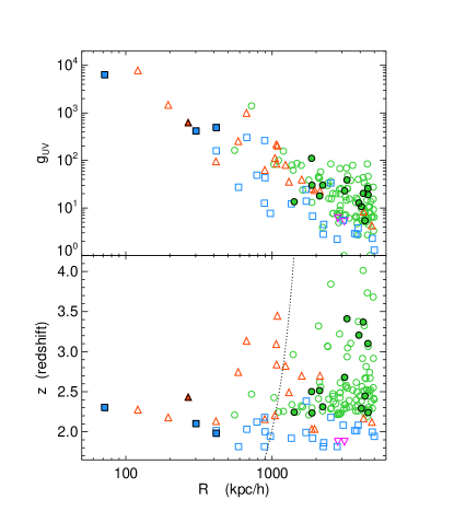
Figure 1.— Distribution of foreground quasar redshifts, transverse separations, and ionizing flux ratios probed by the background quasar sightlines. The upper plot shows the ratio of the ionizing flux to the UV background $g_{\rm UV}$, note the general $R^{-2}$ trend. The lower plot shows foreground quasar redshift versus transverse comoving separations. The (blue) squares have a Keck spectrum of the background quasar, (red) triangles have Gemini background spectra, (magenta) upside down triangles have MMT background spectra, and (green) circles have SDSS background spectra. Filled symbols outlined in black have a super-LLS within $|\Delta v|<1500~{}{\rm km~{}s}^{-1}$ at the foreground quasar redshift (see Table 1) and open symbols have no absorber. The region to the left of the dotted line is excluded by the SDSS fiber collision limit of $\theta=55^{\prime\prime}$, which explains the paucity of SDSS background spectra there. The Keck/Gemini/MMT spectra probe angular separations an order of magnitude smaller than the fiber collision limit, allowing us to study the foreground quasar environment down to down to $70~{}h^{-1}{\rm\ kpc}$ where the ionizing flux is $\sim 10,000$ times the UV background.

Although optically thick absorption line systems, that is Lyman Limit Systems (LLSs) and damped Lyman-$\alpha$ systems (DLAs), are detected as the strongest absorption lines in quasar spectra, the two types of objects, quasars and absorbers, play rather different roles in the evolution of structure in the Universe. The hard ultraviolet radiation emitted by luminous quasars gives rise to the ambient extragalactic ultraviolet (UV) background (see e.g. Haardt & Madau 1996; Miralda-Escudé 2003; Meiksin 2005) responsible for maintaining the low neutral fraction of hydrogen ($\sim 10^{-6}$) in the intergalactic medium (IGM), established during reionization. However, high column density absorbers represent the rare locations where the neutral fractions are much larger. Gas clouds with column densities $\log N_{\rm HI}>17.2$ are optically thick to Lyman continuum ($\tau_{\rm LL}\gtrsim 1$) photons, giving rise to a neutral interior self-shielded from the extragalactic ionizing background. In particular, the damped Ly$\alpha$ systems dominate the neutral gas content of the Universe (Prochaska et al. 2005), which is the primary reservoir for the formation of stars observed in local galaxies.

One might expect optically thick absorbers to be absent at small separations from luminous quasars. For example, a quasar at $z=2.5$ with magnitude $r=19$, emits a flux of ionizing photons that is 130 times higher than that of the extragalactic UV background at an angular separation of $60^{\prime\prime}$, corresponding to a proper distance of 340 $h^{-1}{\rm\ kpc}$. Indeed, the decrease in the number of optically thin absorption lines ($\log N_{\rm HI}<17.2$ hence $\tau_{\rm LL}\lesssim 1$), in the vicinity of quasars, known as the proximity effect (Bajtlik et al. 1988), provides a measurement of the UV background (Scott et al. 2000). If Nature provides a nearby background quasar sightline, one can also study the transverse proximity effect, which is the expected decrease in absorption in a background quasar’s Ly$\alpha$ forest, caused by the transverse ionizing flux of a foreground quasar. The transverse effect has yet to be detected, in spite of many attempts (Crotts 1989; Dobrzycki & Bechtold 1991; Fernandez-Soto, Barcons, Carballo, & Webb 1995; Liske & Williger 2001; Schirber, Miralda-Escudé, & McDonald 2004; Croft 2004, but see Jakobsen et al.2003).

On the other hand, it has long been known that quasars are associated with enhancements in the distribution of galaxies (Bahcall, Schmidt, & Gunn 1969; Yee & Green 1984, 1987; Bahcall & Chokshi 1991; Smith, Boyle, & Maddox 2000; Brown, Boyle, & Webster 2001; Serber et al. 2006; Coil et al. 2006), although these measurements of quasar galaxy clustering are mostly limited to low redshifts $\lesssim 1.0$. Recently, Adelberger & Steidel (2005), measured the clustering of Lyman Break Galaxies (LBGs) around luminous quasars in the redshift range ($2\lesssim z\lesssim 3.5$), and found a best fit correlation length of $r_{0}=4.7~{}h^{-1}{\rm\ Mpc}$ ($\gamma=1.6$), very similar to the auto-correlation length of $z\sim 2-3$ LBGs (Adelberger et al. 2003). Cooke et al. (2006) recently measured the clustering of LBGs around DLAs and measured a best fit $r_{0}=2.9~{}h^{-1}{\rm\ Mpc}$ with $\gamma=1.6$, but with large uncertainties (see also Gawiser et al. 2001; Bouché & Lowenthal 2004). If LBGs are clustered around quasars, and LBGs are clustered around DLAs, might we expect optically thick absorbers to be clustered around quasars? This is especially plausible in light of recent evidence that DLAs arise from a high redshift galaxy population which are not unlike LBGs (Schaye 2001; Møller et al. 2002).

Clues to the clustering of optically thick absorbers around quasars come from proximate DLAs, which have absorber redshifts within $3000~{}{\rm km~{}s}^{-1}$ of the emission redshift of the quasars (see e.g. Møller et al. 1998). Recently, Russell et al. (2006) (see also Ellison et al. 2002), compared the number density of proximate DLAs per unit redshift to the average number density of DLAs in the the Universe (Prochaska et al. 2005). They found that the abundance of DLAs is enhanced by a factor of $\sim 2$ near quasars, which they attributed to the clustering of DLA-galaxies around quasars.

Projected pairs of quasars with small angular separations ($\theta\lesssim 5^{\prime}$) but different redshifts, can also be used to study the clustering of absorbers around quasars. In this context, clustering is manifest as an excess probability, above the cosmic average, of detecting an absorber in the neighboring background quasar spectrum, near the redshift of the foreground quasar. In the first of this series of four papers on optically thick absorbers near quasars (Hennawi et al. 2006, henceforth QPQ1), we used background quasar sightlines to search for optically thick absorption in the vicinity of foreground quasars: 149 projected quasar pairs were systematically surveyed for Lyman limit Systems (LLSs) and Damped Ly$\alpha$ systems (DLAs) in the vicinity of $1.8<z<4.0$ luminous foreground quasars. A sample of 27 new absorbers were uncovered with transverse separations $R<5~{}h^{-1}{\rm\ Mpc}$ (comoving) from the foreground quasars, of which 17 were super-LLSs with $N_{\rm HI}>10^{19}~{}{\rm cm^{-2}}$.

The distribution of foreground quasar redshifts, transverse separations, and ionizing flux ratios probed by the projected pair sightlines studied in QPQ1 are illustrated in Figure 1. The filled symbols outlined in black indicate the sightlines which have an absorption line system with $N_{\rm HI}>10^{19}~{}{\rm cm}^{-2}$ within a velocity interval of $\left|\Delta v\right|=1500~{}~{}{\rm km~{}s}^{-1}$ of the foreground quasar redshift, and the open symbols represent sightlines with no such absorber. The line density of absorbers per unit redshift at $z\sim 2.5$ with column densities $N_{\rm HI}>10^{19}~{}{\rm cm}^{-2}$ is $dN/dz\simeq 0.8$(O’Meara et al. 2006), which implies that the expected number of random quasar-absorber coincidences within $|\Delta v|=1500~{}{\rm km~{}s}^{-1}$ is $\sim 3\%$. The expected number of random quasar-absorber associations in the sample of 149 sightlines is $\langle N\rangle=4.4$; whereas, 17 systems were discovered in QPQ1 – compelling evidence for clustering.

This clustering is particularly conspicuous on small scales: out of 8 sightlines with $R<500~{}h^{-1}{\rm\ kpc}$, 4 quasar-absorber pairs were discovered, which implies a small scale covering factor of $\sim 50\%$, whereas $\langle N\rangle=0.18$ would have been expected at random. This excess of $\sim 25$ over random may not come as a surprise when one considers that galaxies are strongly clustered around quasars on small scales. However, the light from every isolated quasar in the Universe traverses these same small scales on the way to Earth. Naively, we would then expect a comparable covering factor of $N_{\rm HI}>10^{19}~{}{\rm cm}^{-2}$ super-LLSs along the line-of-sight (LOS) – which is definitely not observed to be the case!

How can we quantify the clustering of absorbers around quasars? How do we compare the transverse clustering pattern to the number of proximate absorbers observed along the LOS? What can the quasar-absorber clustering pattern teach us about quasars and absorbers? These questions are addressed in this second paper of the series. We briefly review the QPQ1 survey of projected quasar pairs and discuss the quasar-absorber sample in § 2. A formalism for quantifying the line-of-sight (LOS) and transverse clustering of absorbers around quasars is presented in § 3. In § 4 we introduce a maximum likelihood technique for estimating the quasar-absorber correlation function, which we use to measure the clustering of our quasar-absorber sample in § 5. Our measurement of the transverse clustering is used to predict the expected number of proximate absorption line systems which should be observed along the line-of-sight in § 6. In § 7, we introduce a simple analytical model for the photoevaporation of optically thick absorbers by quasars, which is used to illustrate how comparisons of the line-of-sight and transverse clustering can constrain the distribution of gas in optically thick absorbers. We summarize and discuss our results in § 8

Paper III of this series (Hennawi & Prochaska 2006) investigates fluorescent Ly$\alpha$ emission from our quasar-absorber pairs, and echelle spectra of several of the quasar-LLS systems published here are analyzed in Paper IV (Prochaska & Hennawi 2006). Throughout this paper we use the best fit WMAP (only) cosmological model of Spergel et al. (2003), with $\Omega_{m}=0.270$, $\Omega_{\Lambda}=0.73$, $h=0.72$. Unless otherwise specified, all distances are comoving. It is helpful to remember that in the chosen cosmology, at a redshift of $z=2.5$, an angular separation of $\Delta\theta=1^{\prime\prime}$ corresponds to a comoving transverse separation of $R=20~{}h^{-1}{\rm\ kpc}$, and a velocity difference of $1500~{}{\rm km~{}s}^{-1}$ corresponds to a radial redshift space distance of $s=15~{}h^{-1}{\rm\ Mpc}$. For a quasar at $z=2.5$, with an SDSS magnitude of $r=19$, the flux of ionizing photons is 130 times higher than the ambient extragalactic UV background at an angular separation of $60^{\prime\prime}$ (comoving $R=1.2~{}h^{-1}{\rm\ Mpc}$). Finally, we use the term optically thick absorbers and LLSs interchangeably, both referring to quasar absorption line systems with $\log N_{\rm HI}>17.2$, making them optically thick at the Lyman limit ($\tau_{\rm LL}\gtrsim 1$).

2. Quasar-Absorber Sample

Table 1Super-LLSs Near Quasars from QPQ1

Name	zbg	zfg	$\Delta\theta$	$R$	zabs	$\left|\Delta v\right|$	$\Delta v_{\rm fg}$	$\log N_{\rm HI}$	$g_{\rm UV}$	Telescope
			(′′)	($h^{-1}{\rm\ kpc}$)		(km s-1)	(km s-1)	(cm-2)
SDSSJ0225$-$0739	2.99	2.440	214.0	4310	2.4476	0690	0500	$19.55\pm 0.2$	0005	SDSS
SDSSJ0239$-$0106	3.14	2.308	003.7	0072	2.3025	0540	1500	$20.45\pm 0.2$	6369	Keck
SDSSJ0256$+$0039	3.55	3.387	179.0	4195	3.387	0020	1000	$19.25\pm 0.25$	0020	SDSS
SDSSJ0338$-$0005	3.05	2.239	073.5	1415	2.2290	0960	1500	$20.9\pm 0.2$	0013	SDSS
SDSSJ0800$+$3542	2.07	1.983	023.1	0415	1.9828	0040	0300	$19.0\pm 0.15$	0488	Keck
SDSSJ0833$+$0813	3.33	2.516	103.4	2112	2.5050	0980	1000	$19.45\pm 0.3$	0018	SDSS
SDSSJ0852$+$2637	3.32	3.203	170.9	3917	3.2110	0550	1500	$19.25\pm 0.4$	0013	SDSS
SDSSJ1134$+$3409	3.14	2.291	209.2	4073	2.2879	0320	500	$19.5\pm 0.3$	0011	SDSS
SDSSJ1152$+$4517	2.38	2.312	113.4	2216	2.3158	0370	500	$19.1\pm 0.3$	0030	SDSS
SDSSJ1204$+$0221	2.53	2.436	013.3	0267	2.4402	0370	1500	$19.7\pm 0.15$	0625	Gemini
SDSSJ1213$+$1207	3.48	3.411	137.8	3246	3.4105	0030	1500	$19.25\pm 0.3$	0039	SDSS
SDSSJ1306$+$6158	2.17	2.111	016.3	0302	2.1084	0200	300	$20.3\pm 0.15$	0420	Keck
SDSSJ1312$+$0002	2.84	2.671	148.5	3129	2.6688	0200	500	$20.3\pm 0.3$	0023	SDSS
SDSSJ1426$+$5002	2.32	2.239	235.6	4529	2.2247	1330	500	$20.0\pm 0.15$	0019	SDSS
SDSSJ1430$-$0120	3.25	3.102	200.0	4517	3.1150	0960	1500	$20.5\pm 0.2$	0026	SDSS
SDSSJ1545$+$5112	2.45	2.240	097.6	1873	2.2430	0320	500	$19.45\pm 0.3$	0030	SDSS
SDSSJ1635$+$3013	2.94	2.493	091.4	1861	2.5025	0820	500	$>19$	0111	SDSS

Note. — Optically thick absorption line systems near foreground quasars. The background and foreground quasar redshifts are denoted by $z_{\rm bg}$ and $z_{\rm fg}$, respectively. The angular separation of the quasar pair sightlines is denoted by $\Delta\theta$, which corresponds to a transverse comoving separation of $R$ at the foreground quasar redshift. Absorber redshift is indicated by $z_{\rm abs}$, and $\left|\Delta v\right|$ is the velocity difference between the absorber redshift and our best estimate of the redshift of the foreground quasar. Our estimated error on the foreground quasar redshift is denoted by $\Delta v_{\rm fg}$. Foreground quasar redshifts and redshift errors were estimated according to the detailed procedure described in § 4 of QPQ1. The logarithm of the column density of the absorber from a fit to the H I profile is denoted by $\log N_{\rm HI}$. The column labeled “Telescope” indicates the instrument used to observe the background quasar. The quantity $g_{\rm UV}=1+F_{\rm QSO}/F_{\rm UVB}$ is the maximum enhancement of the quasars ionizing photon flux over that of the extragalactic ionizing background at the location of the background quasar sightline, assuming that the quasar emission is isotropic (see Appendix A of QPQ1). We compare to the UV background computed by F. Haardt & P. Madau (2006, in preparation)

In this section we briefly summarize the quasar-absorber sample and the parent sample of projected pairs from which it was selected; for full details see QPQ1. In § 5 we will quantify the clustering of absorbers around quasars in the transverse direction by comparing the number of quasar-absorber pairs discovered to the number from random expectation. Although lower column density systems were published in QPQ1, we focus here on absorbers with $N_{\rm HI}>10^{19}{\rm cm}^{-2}$, or so called super-LLSs. This choice reflects a variety of concerns. First, we wanted to maximize the number of quasar-absorber pairs – had we restricted consideration to only DLAs we would have been left with 5 systems. Second, this is the lowest column density at which we believe we can identify a statistical sample of absorbers with the moderate resolution spectra used in QPQ1. Finally, the column density distribution of optically thick absorption line systems has been determined for $\log N_{\rm HI}>19$ (Péroux et al. 2005; O’Meara et al. 2006); whereas, it is unknown at the lower column densities $17.2\lesssim\log N_{\rm HI}\lesssim 19$.

Modern spectroscopic surveys select against close pairs of quasars because of fiber collisions. For the Sloan Digital Sky Survey (SDSS), the finite size of optical fibers implies only one quasar in a pair with separation $<55^{\prime\prime}$ can be observed spectroscopically on a given plate, and a slightly smaller limit ($<30^{\prime\prime}$) applies for the Two Degree Field Quasar Survey (2QZ) (Croom et al. 2004). Thus, for sub-arcminute separations, additional spectroscopy is required both to discover companions around quasars and to obtain spectra of sufficient quality to search for absorption line systems. For wider separations, projected quasar pairs can be found directly in the SDSS spectroscopic quasar catalog. Hennawi et al. (2006a) used the 3.5m telescope at Apache Point Observatory (APO) to spectroscopically confirm a large sample of photometrically selected close quasar pair candidates, and published the largest sample of projected quasar pairs in existence.

In QPQ1 we combined high signal-to-noise ratio (SNR) moderate resolution spectra of the closest Hennawi et al. (2006a) projected pairs, obtained from Gemini, Keck, and the Multiple Mirror Telescope (MMT), with a large sample of wider separation pairs, from the SDSS spectroscopic survey. The Keck, Gemini, and MMT spectra were all of sufficient signal-to-noise ratio to detect absorbers with column densities $N_{\rm HI}>10^{19}{\rm cm}^{-2}$, and a SNR criterion was used to isolate the SDSS projected pair sightlines for which such an absorber could be detected in the background quasar spectrum. We considered all projected quasar pair sightlines which had a comoving transverse separation of $R<5~{}h^{-1}{\rm\ Mpc}$, a redshift separation $\Delta v>2500~{}{\rm km~{}s}^{-1}$ between the foreground and background quasar (to exclude physical binaries), and which satisfied our SNR criteria, and arrived at a total of 149 projected pair sightlines in the redshift range $1.8<z<4.0$.

A systematic search for optically thick absorbers with redshifts within $|\Delta v|<1500~{}{\rm km~{}s}^{-1}$ of the foreground quasars was conducted by visually inspecting the 149 projected pair sightlines, where the velocity window was chosen to bracket the uncertainties in the foreground quasars’ systemic redshift (see e.g. Richards et al. 2002, and § 4 of QPQ1). Voigt profiles were fit to systems with significant Ly$\alpha$ absorption to determine the H I column densities. We uncovered 27 new quasar absorber pairs with column densities $17.2<\log N_{\rm HI}<20.9$ and transverse comoving distances $71~{}h^{-1}{\rm\ kpc}<R<5~{}h^{-1}{\rm\ Mpc}$ from the foreground quasars, of which 17 were super-LLSs with $\log N_{\rm HI}>19$. The mean redshift of the foreground quasar in the parent sample was $\langle z\rangle=2.47$ and that of the 17 quasar-super-LLS pairs was $\langle z_{\rm abs}\rangle=2.55$.

The completeness and false positive rate of the QPQ1 survey are a significant source of concern. Prochaska et al. (2005) demonstrated that the spectral resolution (FWHM $\simeq 150~{}{\rm km~{}s}^{-1}$) and SNR of the SDSS spectra are well suited to constructing a complete ($\gtrsim 95\%$) sample of DLAs ($\log N_{\rm HI}>20.3$) at $z>2.2$; however, the completeness at the lower column densities $\log N_{\rm HI}>19$, considered here has not been systematically quantified. Furthermore, aggressive SNR criteria were employed in QPQ1 in order to gather a sufficient number of projected quasar pairs. Line-blending can significantly depress the continuum near the Ly$\alpha$ profile and mimic a damping wing, biasing column density measurements high or giving rise to false positives. Any statistical study will thus suffer from a ‘Malmquist’-type bias because line-blending biases lower column densities upward, and the line density of absorbers $dN/dz$, is a steep function of column density limit.

Based on visually inspecting the 149 background quasar spectra and a comparison with echelle data for three systems, we estimated that the QPQ1 survey was $\sim 90\%$ complete for $\log N_{\rm HI}>19.3$ for all the Keck/Gemini/MMT spectra and $\sim 3/4$ of the SDSS spectra, which accounts for about 125 of the 149 spectra searched. To address the false positive rate, we compared with echelle data for three systems and found that our column density was overestimated by $\sim 2.5\sigma$ for one system, raising it above the super-LLS ($\log N_{\rm HI}>19$) threshold. However, this absorber was located blueward of the quasars Ly$\beta$ emission line, in a part of the spectrum ‘crowded’ by the presence of both the Ly$\alpha$ and Ly$\beta$ forests. A more careful examination of the completeness and false positive rate of super-LLSs identified in spectra of the resolution and SNR used in QPQ1 is definitely warranted. In § 5 we explore how our clustering measurement changes if we discard systems within $\approx 1\sigma$ of the $\log N_{\rm HI}=19$ threshold.

Relevant quantities for the super-LLS-quasar pairs which are used in our clustering analysis are given in Table 1. The distribution of foreground quasar redshifts, transverse separations, and ionizing flux ratios probed by all of our projected pair sightlines is illustrated in Figure 1. The filled symbols outlined in black indicate the sightlines which have an absorption line system near the foreground quasar with $\log N_{\rm HI}>19$ (see Table 1) and open symbols are sightlines with no such absorber.

3. Quantifying Quasar-Absorber Clustering

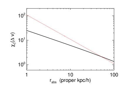
Figure 2.— Dependence of line-of-sight correlation function on the (proper) size of the absorber cross section $r_{\rm abs}$. A velocity interval of $\Delta v=3000~{}~{}{\rm km~{}s}^{-1}$ was assumed. Small cross-sections sample smaller scales near the quasar where the correlation $\xi_{\rm QA}\propto r^{-\gamma}$ function is large, giving a larger value for the average in eqn. (5) for $\chi_{\parallel}$; whereas, large cross-sections dilute $\xi_{\rm QA}$ in the average, giving smaller values of $\chi_{\parallel}$. The solid (black) line is for a correlation length of $r=4.7~{}h^{-1}{\rm\ Mpc}$ and slope of $\gamma=1.6$. The dotted (red) line is for a correlation function with slope $\gamma=2.0$, normalized to the have the same clustering amplitude as the the shallower $\gamma=1.6$ model at $r=1~{}h^{-1}{\rm\ Mpc}$.

In the absence of clustering, the line density of absorption line systems per unit redshift above the column density threshold $N_{\rm HI}$ is given by the cosmic average

$$\left\langle\frac{dN}{dz}\right\rangle(>N_{\rm HI},z)=nAf_{\rm cov}\frac{c}{H(z)},$$ (1)

where $n$ is comoving number density of the galaxies or objects which give rise to absorption line systems, $A$ is their absorption cross section (in comoving units), $f_{\rm cov}$ is the covering factor, and $H(z)$ is the Hubble constant. Note that the line density is degenerate with respect to the combination $nAf_{\rm cov}$ and only their product can be determined by measuring the abundance of absorption line systems.

At an average location in the Universe, the probability of finding a absorber in a background quasar spectrum within the redshift interval $\Delta z=2(1+z)\Delta v/c$, corresponding to a velocity interval $2\Delta v$ is simply $P=\langle dN/dz\rangle\Delta z$. For a projected pair of quasars, clustering around the foreground quasar will increase the probability of finding an absorber in the background quasar spectrum in the vicinity of the foreground quasar; whereas, the foreground quasars radiation field could reduce this enhancement by photoevaporating absorption systems. If the quasar sightlines have a comoving transverse separation $R$, and assuming that one searches a velocity interval $\pm\Delta v$ about the foreground quasar redshift (because of redshift uncertainties), we can express the increase in line density near the foreground grounds in terms of a transverse correlation function $\chi_{\rm\perp}(R)$ as

$$\frac{dN}{dz}=\left\langle\frac{dN}{dz}\right\rangle\left[1+\chi_{\perp}(R,\Delta v)\right]$$ (2)

where $\chi_{\rm\perp}(R,\Delta v)$ is given by an average of the 3-d quasar-absorber correlation function, $\xi_{\rm QA}(r)$, over a cylinder with volume $V=A[2\Delta v/aH(z)]$. Here, $a$ is the scale factor and $2\Delta v(1+z)/H(z)$ is the length of the cylinder in the LOS direction. We can thus write

$$\chi_{\perp}(R) = \frac{1}{V}\int_{\rm V}dV~{}\xi_{\rm QA}(r)$$

$$\approx \frac{aH(z)}{2\Delta v}\int_{\frac{-\Delta v}{aH(z)}}^{\frac{\Delta v}{aH(z)}}dZ~{}\xi_{\rm QA}(\sqrt{R^{2}+Z^{2}}),$$

where $Z$ is a comoving distance in redshift space. The last approximation in eqn. 3 assumes that the volume average over the cylinder can be replaced by the line average along the line-of-sight direction, which is valid provided that we are in the ‘far-field’ limit, i.e., the transverse separation is much larger than the diameter of the cylinder $R\gg{\sqrt{A}}$. Thus provided we consider distances $R$ much larger than the dimension of the absorber, the transverse clustering is independent of the absorption cross-section.

For proximate absorbers along the line of sight, we can similarly define a line-of-sight correlation function

$$dN/dz=\langle dN/dz\rangle[1+\chi_{\parallel}(\Delta v)]$$ (4)

where

$$\chi_{\parallel}(\Delta v)=\frac{aH(z)}{A\Delta v}\int_{Z_{\rm cut}}^{\frac{\Delta v}{aH(z)}}dZ\int dA~{}\xi_{\rm QA}(r).$$ (5)

The lower limit of the radial integration is set to $Z_{\rm cut}$, a cutoff which is introduced to parametrize our ignorance of the geometry of the absorbers. For instance, if the absorbers were pancake shapes which were always oriented perpendicular to the line of sight (like face-on spiral galaxies) then we would not cutoff the line-of-sight integration at all ($Z_{\rm cut}=0$), since face on pancakes at zero separation can still obscure the quasar. For ’hard sphere’, we would set $Z_{\rm cut}=2\sqrt{A/\pi}$ — presuming that the obscuring cross-section of the absorber drops to zero for points interior to it. As smaller values of $Z_{\rm cut}$ will correspond to larger line-of-sight clustering, we henceforth conservatively assume the hard sphere case and use $Z_{\rm cut}=2\sqrt{A/\pi}$

Note that one is no longer in the ‘far-field’ limit for the integral in eqn. (5), and the clustering amplitude $\chi_{\parallel}$ explicitly depends on the cross section of the absorber. It is easy to understand the nature of this dependence if one considers that the line density $\propto nA$ is fixed by measurements of $\langle dN/dz\rangle$. Thus, smaller cross-sections correspond to larger volume number densities, but smaller scales near the quasar are being sampled by the integral in eqn. (5), where the correlation $\xi_{\rm QA}\propto r^{-\gamma}$ function is large. Conversely, larger cross-sections sample regions further from the quasar, and thus $\xi_{\rm QA}$ is averaged over a larger volume and hence diluted. Figure 2 illustrates the dependence of $\chi_{\parallel}(\Delta v)$ on the proper radius of the absorber cross section, $r_{\rm abs}$, for a range of sizes.

In eqns. (3) and (5) $\xi_{\rm QA}(r)$ represents a real space correlation function and it may appear that we have neglected redshift space distortions. Strictly speaking, the redshift space correlation function $\xi_{\rm QA}(R,Z)$, should be appear in eqns. 3 and 5. This $\xi_{\rm QA}(R,Z)$ is the convolution of the real space correlation function $\xi(r)$, with the velocity distribution in the radial direction, which can have contributions from both peculiar velocities and uncertainties in the systemic redshifts of the quasar. However, provided that the distance in redshift space over which we project $\Delta v$ contains most of the probability under this distribution, it is a good approximation to replace the redshift space correlation function, under the integrals in eqns. (3) and (5), with the real space correlation function, because radial velocities will simply move pairs of points within the volume.

4. Estimating the Correlation Function

4.1. Maximum Likelihood Estimator

Given a quasar-absorber correlation function $\xi_{\rm QA}$, eqns. (2) and (3) describe how to compute the probability of finding an absorber in the redshift interval $\Delta z=2(1+z)\Delta v/c$ at a transverse distance $R$ from a foreground quasar: $P(R,z)=(dN/dz)\Delta z$. Considering that we only have 17 quasar-absorber pairs selected from 149 sightlines, it will be difficult to measure more than a single parameter with reasonable errors. Hence, we assume the quasar-absorber correlation function to have a power-law form

$$\xi_{\rm QA}=C\left(\frac{r}{r_{0}}\right)^{-\gamma},$$ (6)

where $C$ is a clustering amplitude and $r_{0}$ is the correlation length. The amplitude $C$ is degenerate with $r_{0}$, but we choose to estimate $C$, because it allows for the possibility of anti-correlation ($C<0$) which could result from the QSO ionizing radiation field. Motivated by the the slope of the LBG auto-correlation function (Adelberger et al. 2005a), we choose to fix $\gamma=1.6$. A similar procedure was employed by (Adelberger & Steidel 2005, henceforth AS05), who measured clustering of LBGs around luminous quasars ($2\lesssim z\lesssim 3.5$), and found a best fit correlation length of $r_{0}=4.7~{}h^{-1}{\rm\ Mpc}$. We set $r_{0}=4.7~{}h^{-1}{\rm\ Mpc}$ as a fiducial value; thus $C$ can be interpreted as the quasar-absorber clustering amplitude relative to the AS05 quasar-LBG result.

Consider an ensemble of $N$ projected pair sightlines with background quasars at transverse separations $R_{i}$ from foreground quasars at redshifts $z_{i}$. Given $\xi_{QA}$, we can compute the associated probabilities $P_{i}\equiv P(R_{i},z_{i})$. Suppose that $N_{\rm SLLS}$ of these $N$ sightlines show absorption from super-LLSs with $\log N_{\rm HI}>19$. The likelihood of the data, given the model parameter $C$ is then

$$\mathcal{L}(C)=\prod_{i}^{N_{\rm SLLS}}P_{i}\prod_{j}^{N-N_{\rm SLLS}}(1-P_{j}),$$ (7)

where the probabilities $P_{i}\leq 1$ are capped at 1. By maximizing the likelihood with respect to the parameter $C$, we estimate the clustering amplitude from the data.

4.2. Monte-Carlo Simulations

We must verify that the maximum likelihood estimator in eqn. (7) is unbiased, and we would also like to know how to assign error bars to an estimate of $C$. Both of these points can be addressed with monte-carlo methods. The distribution of redshifts and transverse separations in Figure 1 is not uniform, and it is thus important that we preserve this distribution when constructing mock data sets to assign errors.

For a ‘true’ value of the clustering amplitude $C$, we can compute the probabilities $P_{i}\equiv P(R_{i},z_{i})$ of observing an absorber for each of the $N$ projected pair sightlines. Mock data sets can then be constructed by generating an $N$-dimensional vector of deviates from the uniform distribution $x_{i}$, and assigning sightlines with $x_{i}<P_{i}$ an absorption line system. The same maximum likelihood estimator is applied to these mock data sets to determine an estimate ${\hat{C}}$ for each one, thus allowing us to measure the probability distribution $P({\hat{C}}|C)$ of the estimate about the true model.

4.3. Binned Correlation Function

An alternative to the maximum likelihood technique described above, would be to estimate the correlation length by fitting a power-law model to estimates of the correlation function in bins of transverse separation. However, because we have only 17 quasar-absorber pairs, the best-fit correlation length from this procedure would be very sensitive to the binning chosen. We compute the correlation function in bins because it provides a useful way to visualize the data, although we do not fit the binned data for $C$

A simple estimator for the transverse correlation function in eqn. (2) is

$$\chi_{\perp}(R,\Delta v)=\frac{\langle{\rm QA}\rangle}{\langle{\rm QR}\rangle}-1,$$ (8)

where $\langle{\rm QA}\rangle$ is the number of quasar-absorber pairs in a transverse radial bin centered on $R$, and $\langle{\rm QR}\rangle=\sum_{i}\langle dN/dz\rangle\Delta z$, is the number of quasar-random pairs expected.

4.4. The Column Density Distribution

Before we can estimate the correlation amplitude with eqn. (7), we require the cosmic average line density of super-LLSs $\langle dN/dz\rangle$. The line density is the zeroth moment of the column density distribution

$$\left\langle\frac{dN}{dz}\right\rangle(>N_{\rm HI},z)=\int_{N_{\rm HI}}^{\infty}f_{\rm HI}(N_{\rm HI},z)dN_{\rm HI}.$$ (9)

O’Meara et al. (2006) measured the column density distribution for super-LLSs in the range $19<\log N_{\rm HI}<20.3$ at $z\sim 2.7$ and found good agreement with a power law $f(N)=A(N_{\rm HI}/10^{19}~{}{\rm cm^{-2}})^{b}$, where $A=1.10\times 10^{-20}$ and $b=-1.43$. For $\log N_{\rm HI}>20.3$, (Prochaska et al. 2005) measured the column density distribution from the SDSS quasar sample in redshift bins.

To evaluate the integral in eqn. (9), we use the O’Meara et al. (2006) power law fit in the range $19<\log N_{\rm HI}<20.3$, and a spline fit to the Prochaska et al. (2005) results in the redshift bin centered at $z\sim 2.7$. For the redshift evolution, we simply scale the line density of all absorbers by the evolution of DLAs $\log N_{\rm HI}>20.3$ measured by Prochaska et al. (2005) (see their Figure 8). This procedure assumes that the abundance of super-LLSs evolves similarly to that of DLAs, an assumption that is consistent with but not confirmed by O’Meara et al. (2006).

5. Clustering Results

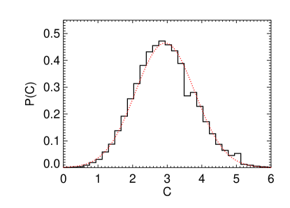
Figure 3.— Distribution of clustering amplitude estimates from monte-carlo simulations. The black histogram shows the probability distribution of the clustering amplitude maximum likelihood estimates $P({\hat{C}})$, for a model with true value equal to our measurement of $C=2.9$. This distribution was created by applying the maximum likelihood estimator in eqn. (7) to 100,000 mock realizations of our 149 projected pair sightlines, as described in § 4.2. The mean of this distribution is $\langle{\hat{C}}\rangle=2.94$, the dispersion is $\sigma=0.86$, and the (red) dotted curve shows a Gaussian with the same mean and dispersion. The full distribution (black histogram) is used to assign errors to our measurement.

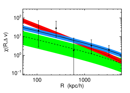
Figure 4.— Binned transverse quasar-absorber correlation function for 17 quasar-absorber pairs selected from 149 projected pair sightlines. The lines indicate the best-fit model from our maximum likelihood analysis and the shaded regions indicate the range allowed by $1\sigma$ errors estimated from monte-carlo simulations. The solid line and the blue shaded region are for an assumed correlation function slope of $\gamma=1.6$. The steeper dotted line and red shaded region are for $\gamma=2.0$. The dashed curve and green region show the transverse correlation function $\chi_{\perp}$ if we set the quasar-absorber correlation function $\xi_{\rm QA}$ to the QSO-LBG correlation function measured by AS05 ($r_{0}=4.7\pm 1.3~{}h^{-1}{\rm\ Mpc};\gamma=1.6$)

We applied the maximum likelihood estimator to the 17 quasar-absorber pairs (see Table 1) selected from the 149 projected pair sightlines shown in Figure 1. The maximum likelihood value of the clustering amplitude is $C=2.9$, which corresponds to a correlation length of $r_{0}=9.2~{}h^{-1}{\rm\ Mpc}$.

In Figure 3 we show the probability distribution of the clustering amplitude maximum likelihood estimates $P({\hat{C}})$, for a model with true value equal to our measurement of $C=2.9$. This distribution was created by applying the maximum likelihood estimator in eqn. (7) to 100,000 mock realizations of our 149 projected pair sightlines, as described in § 4.2. The mean of this distribution is $\langle{\hat{C}}\rangle=2.94$, the dispersion is $\sigma=0.86$, and the (red) dotted curve shows a Gaussian with the same mean and dispersion. The monte-carlo simulation indicates that our estimator is indeed unbiased and that the error distribution is reasonably well approximated by a Gaussian. Using the full distribution from the monte-carlo simulation, we compute the $68\%$ confidence interval about the ‘true’ input value, which we use to quote errors on our clustering measurement: $C=2.9\pm 0.8$, or $r_{0}=9.2^{+1.5}_{-1.7}~{}h^{-1}{\rm\ Mpc}$. If we assume a steeper slope for the correlation function $\gamma=2$, we obtain $r_{0}=5.8^{+1.0}_{-0.6}~{}h^{-1}{\rm\ Mpc}$.

We detect strong clustering of super-LLSs around quasars. Figure LABEL:fig:clust shows the binned transverse correlation function $\chi_{\perp}$ compared to the two maximum likelihood fits ($\gamma=1.6$ and $\gamma=2$) and to the prediction from the quasar-LBG correlation function measured by AS05. For $\gamma=1.6$, the quasar-absorber clustering amplitude is three times larger than the quasar-LBG measurement of AS05 and inconsistent with it at the $\gtrsim 1\sigma$ level.

The auto-correlation functions of high redshift galaxies tend to become progressively steeper on (comoving) scales $R\lesssim 1~{}h^{-1}{\rm\ Mpc}$ characteristic of the sizes of dark matter halos (Coil et al. 2005; Ouchi et al. 2005; Lee et al. 2006; Conroy06), thus similar behavior might be in cross-correlation around quasars. Indeed, Hennawi et al. (2006a) detected an order of magnitude excess quasar auto-clustering on scales $\lesssim 100~{}h^{-1}{\rm\ kpc}$. For this reason, we also quote our results for $\gamma=2$, although a steeper slope is not clearly favored by the binned data in Figure 4.

At first glance, it may seem odd that the relative error on our measurement of $r_{0}$ is $\sim 20\%$ using only 17 quasar-absorber pairs; whereas AS05 quote a $\sim 30\%$ error on $r_{0}$ from $\sim 200$ quasar-LBG pairs around a sample of $\sim 50$ quasars. The estimator used here is qualitatively similar to that used by AS05 (see also Adelberger et al. 2005a) in that both techniques rely on the radial clustering of pairs of objects at fixed angular positions, because the angular selection functions are unknown (see Adelberger 2005b). It is thus worth explaining that our smaller errors arise from a few factors.

First, the relative error decreases with clustering amplitude, and our best fit has a factor of three larger clustering strength. Second, AS05 exclude scales $R\lesssim 1.2~{}h^{-1}{\rm\ Mpc}$ from their analysis; whereas four out of our 17 quasar-absorber pairs have $R<1.2~{}h^{-1}{\rm\ Mpc}$. Small scale pairs are effectively ‘worth’ many large scale pairs because the signal to noise per pair is much higher. Finally, the AS05 errors are determined from the field to field dispersion in the data, which includes a contribution from cosmic variance. Because the projected pairs of quasars are distributed over the entire sky, our measurement does not suffer from cosmic variance errors.

To illustrate that the errors from our monte-carlo technique are sensible and comparable to the AS05 result, we randomly resampled our pair sightlines with $R>1.2~{}h^{-1}{\rm\ Mpc}$ to create a mock projected pair sample 30 times larger, but with the same distribution of redshifts and transverse distances. We increased the search window $\Delta v=3000~{}~{}{\rm km~{}s}^{-1}$, in closer agreement with the $l=30~{}h^{-1}{\rm\ Mpc}$ radial window averaged over by AS05. The average number of quasar-absorber pairs expected from this hypothetical enlarged sample is $\langle N\rangle=\sum_{i}P_{i}=206$, which is of order the number of LBG-AGN pairs used by AS05. Assuming $\gamma=1.6$ and $r_{0}=4.7~{}h^{-1}{\rm\ Mpc}$, our monte-carlo simulation gives $r_{0}=4.7^{+0.9}_{-1.0}~{}h^{-1}{\rm\ Mpc}$, or a relative error of $\sim 20\%$, comparable to the AS05 errors but slightly smaller.

5.1. Systematic Errors

5.1.1 ‘Malmquist’ Bias

As discussed in § 2, the identification of $\log N_{\rm HI}=19$ in spectra at the SNR and resolution used in QPQ1, can result in a significant ‘Malmquist’ type bias because line-blending scatters lower column density absorbers upward, and the line density of absorbers $dN/dz$, is a steep function of column density limit. If absorbers with column densities $\log N_{\rm HI}<19$ scatter up into our sample, this error would bias our clustering measurement high. To investigate the impact of this bias, we redo the clustering analysis but ignoring the six quasar-absorber pairs in Table 1 which have column densities within $1\sigma$ of the threshold $logN_{\rm HI}=19$: SDSSJ 0256$+$0039, SDSSJ 0800$+$3542, SDSSJ 0852$+$2637’, SDSSJ 1152$+$4517, SDSSJ 1213$+$1207, and SDSSJ 1635$+$3013. The eleven remaining quasar-absorber pairs give a maximum likelihood clustering amplitude of $C=1.7\pm 0.7$ or $r_{0}=6.4^{+1.7}_{-1.8}~{}h^{-1}{\rm\ Mpc}$, compared to our measurement of $C=2.9\pm 0.8$, or $r_{0}=9.2^{+1.5}_{-1.7}~{}h^{-1}{\rm\ Mpc}$ for the full sample. This illustrates that even under very conservative assumptions about the possible effect of Malmquist bias, the clustering amplitude would be only be reduced by $\sim 1.5\sigma$.

5.1.2 Redshift Errors

Another possible source of bias in our sample could arise from the determination of the foreground quasar redshifts. Note that the clustering analysis properly takes the redshift uncertainties into account, by averaging the correlation function over a window of $|\Delta v|=1500~{}~{}{\rm km~{}s}^{-1}$. However, assigning redshifts to the foreground quasar (see § 4 of QPQ1) is not a completely objective process. The quasar emission lines sometimes exhibit mild-BAL or metal line absorption, and the line centering can be sensitive to how these features are masked. It is possible that we were biased towards including quasar-absorber pairs in our sample, and thus tended to assign redshifts resulting in velocity differences $|\Delta v|<1500~{}~{}{\rm km~{}s}^{-1}$. To address this issue we redo the analysis discarding the three quasar-absorber pairs in Table 1 which have velocity differences larger than the quoted error, $\Delta v_{\rm fg}>|\Delta v|$: SDSSJ 0225$-$0739, SDSSJ 1426$+$5002, and SDSSJ 1635$+$3013. The 14 remaining quasar-absorber pairs give a maximum likelihood clustering amplitude of $C=2.4^{+0.8}_{-0.7}$ or $r_{0}=8.1^{+1.6}_{1.7}~{}h^{-1}{\rm\ Mpc}$. Furthermore, if we discard the five quasar-absorber pairs with the largest velocity differences, we measure $C=1.9\pm 0.7$ or $r_{0}=7.1^{+1.6}_{-1.7}~{}h^{-1}{\rm\ Mpc}$. Thus we conclude that even if we were biased towards including several quasar-absorber pairs with the velocity differences $|\Delta v|>1500~{}~{}{\rm km~{}s}^{-1}$, this would only reduce the the measured clustering amplitude by $\sim 1\sigma$.

6. Anisotropic Clustering of Absorbers Around Quasars

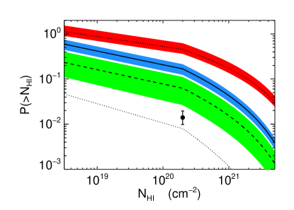
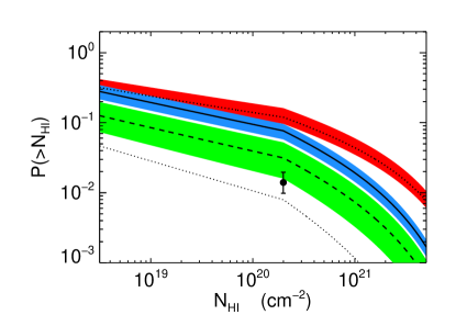
Figure 5.— Probability of a quasar at $z\sim 2.5$ having a proximate absorber within $3000~{}~{}{\rm km~{}s}^{-1}$ as a function of limiting column density. The left panel is for ‘small’ absorber cross sections and the right panel is for ‘large’ absorbers. Our measurement of the quasar-absorber correlation function $\xi_{\rm QA}$ from the transverse direction is used to predict the number of proximate absorbers along the line-of-sight. The curves and shaded regions show the predictions and $1\sigma$ errors for the quasar-absorber correlation function $\xi_{\rm QA}$ estimated from the transverse direction in § 5, as well as the clustering strength measured by AS05. The linestyles and colors correspond to the same models as in Figure 4. The lower dotted line indicates the prediction in the absence of clustering, which is just the integral of the column density distribution in eqn. 9. The point with the error bar represents the Russell et al. (2006) measurement for proximate DLAs ($\log N_{\rm HI}>20.3$) at $z\sim 3.4$.

If the clustering pattern of optically thick absorbers around quasars is isotropic, then we can use our estimate of the quasar-absorber correlation function in § 5 to predict the number of ‘proximate’ super-LLSs that should be observed in a given velocity window, $\Delta v$, along the line-of-sight. According to eqn. (5), the clustering enhancement $\chi_{\rm\parallel}$ can be computed by averaging $\xi_{\rm QA}$ over a cylinder of length $\Delta v/aH(z)$ and cross sectional area $A$.

However, because the cross-section of the absorbers is unknown, relating the transverse clustering to the line-of-sight clustering requires an assumption about the size of the cross section. Very little is known about the sizes of DLAs and LLSs. Briggs et al. (1989) detected H I 21cm absorption of a DLA with $N_{\rm HI}=5\times 10^{21}~{}{\rm cm^{-2}}$ against an extended radio source, allowing them to place a lower limit of $r\gtrsim 12~{}h^{-1}{\rm\ kpc}$ on the size of the absorbing region. Prochaska (1999) estimated an absorbing path length of $\sim 2h^{-1}{\rm\ kpc}$ for a super-LLS with $\log N_{\rm HI}=19.1$, by comparing the column density to the total volume density, which was determined from the collisionally excited C II^∗ $\lambda 1335$ transition. Adelberger et al. (2006) constrained the size of a DLA with $\log N_{\rm HI}=20.4$ to be $\gtrsim 8~{}h^{-1}{\rm\ kpc}$, based on their detection of fluorescent Ly$\alpha$ emission from the edge of a DLA-galaxy situated $\sim 8~{}h^{-1}{\rm\ kpc}$ from the location of DLA absorption. Lopez et al. (2005) measured identical column densities of $N_{\rm HI}=10^{20.5}~{}{\rm cm}^{-2}$ for both DLAs at ($z=0.9313$) detected in the individual images of the gravitational lens HE 0512 $-$ 3329, allowing them to constrain the size of the DLA to be $\gtrsim 4h^{-1}{\rm\ kpc}$ Smette et al. (see also 1995). It is not clear how to relate these measurements to the absorption cross sections of the $\log N_{\rm HI}>19$ of interest to us here.

To determine the cross section size as a function of limiting column, $r_{\rm abs}(>N_{\rm HI})\equiv\sqrt{aA(>N_{\rm HI})/\pi}$, we adopt the simple approximation that the comoving number density of absorption line systems, $n$, and the covering factor, $f_{\rm cov}$ are independent of column density, which gives the simple scaling $r_{\rm abs}\propto\sqrt{\langle dN/dz\rangle}$ from eqn. (1). Two families of sizes, ‘small’ and ‘large’ are considered, which we believe bracket the range of possibilities. Fiducial physical sizes of $r_{\rm abs}=5~{}h^{-1}{\rm\ kpc}$ and $r_{\rm abs}=20~{}h^{-1}{\rm\ kpc}$ are chosen at the DLA threshold ($\log N_{\rm HI}>20.3$) for the ‘small’ and ‘large’ absorbers, respectively. The $r_{\rm abs}\propto\sqrt{\langle dN/dz\rangle}$ scaling then predicts respective sizes of $r_{\rm abs}=9~{}h^{-1}{\rm\ kpc}$ and $r_{\rm abs}=38~{}h^{-1}{\rm\ kpc}$ for super-LLSs with $\log N_{\rm HI}>19$.

In Figure 5 we show the probability that a quasar at $z=2.5$ will have a ‘proximate’ optically thick absorption line systems within $\Delta v<3000~{}~{}{\rm km~{}s}^{-1}$, as a function of limiting column density. The left (right) panel shows the prediction for the ‘small’ (‘large’) family of cross-section sizes, and the dot-dashed curves shows the prediction in the absence of clustering ($\chi_{\parallel}=0$), which is simply the integral of the column density distribution in eqn. (9). Since we have measured the transverse clustering only for $\log N_{\rm HI}>19$, this figure assumes that clustering is independent of limiting column density.

The transverse clustering overpredicts the fraction of quasars which have a proximate absorber by a large factor. For example, for ‘small’ absorption cross sections and $\gamma=1.6$, the quasar-absorber correlation function measured from the transverse direction predicts that a fraction $P=0.30\pm 0.07$ of all quasars should show a proximate super-LLS ($\log N_{\rm HI}>19$) within $\Delta v=3000~{}~{}{\rm km~{}s}^{-1}$. Even the AS05 clustering amplitude, which is a factor of $\sim 3$ smaller than our best fit, would predict $P=0.12^{+0.08}_{-0.06}$. A steeper correlation function results in even more proximate absorbers. For the best fit transverse clustering amplitude with $\gamma=2$, the probability would be $P=0.49^{+0.17}_{-0.10}$.

Making the absorbers larger changes this prediction by factors of $\sim 2-3$. The ‘large’ absorbers predict a fraction $P=0.14\pm 0.03$ of quasars should have a proximate absorber, given our best-fit clustering amplitude for $\gamma=1.6$. Our steeper $\gamma=2$ fit gives $P=0.14^{+0.02}_{-0.04}$ and the AS05 result predicts $P=0.07\pm 0.03$ and our steeper $\gamma=2$ fit gives $P=0.14^{+0.02}_{-0.04}$. Although the line density of proximate super-LLSs near quasar has yet to be measured (but see Prochter, Hennawi, & Prochaska 2006), it is incontrovertible that $15-50\%$ percent of quasars do not show a super-LLS within $\Delta v<3000~{}~{}{\rm km~{}s}^{-1}$ along the line of sight.

Russell et al. (2006) recently measured the line density of proximate DLAs ($\log N_{\rm HI}>20.3$) with $\Delta v<3000~{}~{}{\rm km~{}s}^{-1}$ from 731 SDSS quasars. The median redshift of their quasar sample was $z=3.335$ and they found $\langle dN/dz\rangle=0.38^{+0.18}_{-0.08}$. The point with the error bar in Figure 5 indicates the probability of having a proximate DLA from the Russell et al. (2006) measurement, $P_{\rm DLA}=0.013^{+0.006}_{-0.002}$. Our best-fit clustering amplitude predicts that $P=0.12\pm 0.3$ ($P=0.25^{+0.09}_{-0.05}$) of quasars should have a nearby DLA for small absorbers and $\gamma=1.6$ ($\gamma=2$). Large absorbers change this prediction to $P=0.055\pm 0.013$ ($P=0.069^{+0.023}_{-0.013}$) .

The caveat should be included that our prediction for the number of proximate absorbers from the transverse clustering, is very sensitive to the small scale behavior of the correlation function. Specifically, using eqn. 5 to predict the line-of-sight clustering implicitly assumes that the power law model of the correlation function $\xi\propto r^{-\gamma}$, is valid down the lower limit of the integration, $Z_{\rm cut}$, which we have set to be the diameter of the absorbers. For super-LLSs, we used (proper) radii of $r_{\rm abs}=9~{}h^{-1}{\rm\ kpc}$ and $r_{\rm abs}=38~{}h^{-1}{\rm\ kpc}$, for small and large absorbers, respectively, corresponding to (comoving) $Z_{\rm cut}=63$ and $Z_{\rm cut}=266$ at $z=2.5$. The smallest transverse separation of our projected pair sample is $R=72~{}h^{-1}{\rm\ kpc}$, and there are just 5 sightlines with $R\lesssim 300~{}h^{-1}{\rm\ kpc}$, three of which have an absorber (see Figure 1 and Table 1). The transverse measurement assumes a single power law from $R=70~{}h^{-1}{\rm\ kpc}-5~{}h^{-1}{\rm\ Mpc}$. One should bear in mind that only a handful of projected pairs probe the small scales ($R\lesssim 300~{}h^{-1}{\rm\ kpc}$) that the line-of-sight clustering is very sensitive too; but, it is reassuring that closest bin in Figure 4 is consistent with the power law fit.

We have shown that the transverse clustering which we quantified in § 5 overpredicts the abundance of proximate absorbers along the line-of-sight by a large factor $\sim 4-20$, under reasonable assumptions about the sizes of the cross sections of these absorbers. The clustering pattern of absorbers around quasars is thus highly anisotropic. The most plausible explanation for this anisotropy is that the transverse direction is less likely to be illuminated by ionizing photons than the line-of-sight, and that the optically thick absorbers along the line-of-sight are being photoevaporated. We will discuss the physical effects which could give rise to this anisotropy in § 8. Next, we introduce a simple model that provides physical insight into the problem of optically thick absorbers subject to the intense ionizing flux of a nearby quasar.

7. Photoevaporation of Optically Thick Clouds

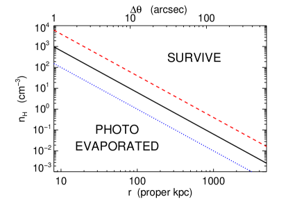
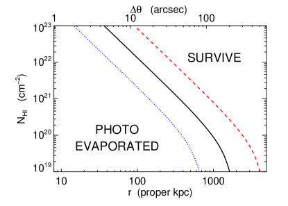
Figure 6.— Regions of parameter space where an optically thick absorber can survive near a luminous quasar set by eqn. 10. The dashed (red), black (solid) and dotted (blue) curves correspond to $r=17$, $19$, & $21$ mag, respectively. Optically thick absorbers above a curve can survive, whereas those below are photoevaporated. Left: Survival regions in the volume density-distance plane, assuming a neutral column of $\log N_{\rm HI}=20.3$. Right: Survival regions in the neutral column density-distance plane, assuming a volume density of $n_{\rm H}=0.1~{}{\rm cm^{-3}}$.

The problem of an optically thick absorption line system exposed to the ionizing flux of a nearby luminous quasar is analogous to that of a neutral interstellar cloud being exposed to the ionizing radiation of an OB star – a problem which was first investigated by Oort & Spitzer (1955). Bertoldi (1989) classified the behavior of photoevaporating clouds based on their initial column density and the ionization parameter at the location of the cloud, and developed an analytical solution to follow the radiation-driven implosion phase of the cloud. Interestingly, although Bertoldi (1989) was primarily concerned with the fate of interstellar clouds near OB stars in H II regions, he commented briefly on the applicability of the same formalism to Ly$\alpha$ clouds exposed to the ionizing flux of a quasar.

7.1. Cloud Zapping

Following Bertoldi (1989), we model an optically thick absorber as a homogeneous spherical neutral gas cloud with total number density of hydrogen $n_{H}$, which is embedded in photoionized intergalactic medium at temperature $T=20,000~{}{\rm K}$, corresponding to an isothermal sound speed $c_{\rm i}=16.5~{}T_{20}^{1/2}~{}~{}{\rm km~{}s}^{-1}$, where $T_{20}$ is the temperature in units of $20,000~{}{\rm K}$. If the cloud is at a distance $r$ from a luminous quasar which is emitting $S$ ionizing photons per second, then the the ionizing flux at the cloud surface, $F_{\rm i}=S/4\pi r^{2}$, will drive an ionization front into the neutral gas. If the flux is large enough to make the conditions R-type (see Spitzer (1978) for a discussion of how ionization fronts are classified), an R-type ionization front will propagate through the cloud without dynamically perturbing the neutral gas. As the front propagates into the cloud, it ionizes an increasing column of neutral gas, steadily reducing the ionizing flux at the front, until the conditions become M-type, at which point the front will stall and drive a shock into the neutral upstream gas. This shock will implode the cloud and compress it until conditions become D-type, allowing the front to continue propagating and establishing a steady photoevaporation flow (Bertoldi 1989).

The cloud will be ‘zapped’, or completely photoevaporated, if the ionizing flux is large enough relative to the column density, such that the entire cloud can be ionized in a recombination time. In this case, the R-type front will completely cross the cloud without stalling. Part of the cloud will remain neutral and a shock will form provided that

$$\delta=494N_{\rm H,20.3}^{-1}\left[\Gamma-1.1\times 10^{-4}~{}T_{\rm 20}^{1/2}\right]<1$$ (10)

where $N_{\rm H,20.3}$ is the total hydrogen column in units of $10^{20.3}~{}{\rm cm^{2}}$, and the ionization parameter is defined by $\Gamma\equiv F_{i}/n_{0}c$ with

$$\Gamma=2.58\times 10^{-5}~{}S_{56}~{}r_{\rm Mpc}^{-2}~{}n_{\rm H,1}^{-1},$$ (11)

where $S_{56}$ is the ionizing flux in units of $10^{56}~{}{\rm s^{-1}}$, $r_{\rm Mpc}$ is the physical distance in units of ${\rm Mpc}$, and $n_{\rm H,1}$ is the total hydrogen number density in units of $1~{}{\rm cm^{-3}}$. The condition that the ionization front be R-type at the surface of the cloud is $\Gamma>1.1\times 10^{-4}T_{20}^{1/2}$.

Consider our fiducial example of a foreground quasar with $r=19$ at an angular separation of $\Delta\theta=1^{\prime}$ from an absorber corresponding to a transverse proper distance of $485~{}{\rm kpc}$. The ionizing flux is enhanced by $g_{\rm UV}=130$ over the UV background and $S_{56}=5.2$. For a DLA with total hydrogen column of $N_{\rm H}=10^{20.3}~{}{\rm cm^{-2}}$ at this distance, the cloud will survive ($\delta<1$) provided $n_{\rm H}>0.27~{}{\rm cm^{-3}}$, which would give $\Gamma<0.002$.

The left panel of Figure 6 shows the lower limits on the volume density of a DLA with neutral hydrogen column $\log N_{\rm HI}=20.3$, set by the condition for cloud survival, as a function of physical distance from a quasar at $z=2.5$. The dashed (red), black (solid) and dotted (blue) curves correspond to $r=17$, $19$, & $21$ mag, respectively. In the region below each curve, the volume densities are too small and the clouds are photoevaporated; whereas, above the curves the clouds can survive. The right panel shows the lower limit on the neutral hydrogen column density as a function of distance, assuming a volume density $n_{\rm H}=0.1$. If DLAs with $\log N_{\rm HI}=20.3$ have sizes in the range $r_{\rm abs}\sim 1-5~{}{\rm kpc}$ their corresponding number densities are $n_{\rm H}\sim N_{\rm H}/r_{\rm abs}=0.01-1$. Thus according to Figure 6 optically thick absorbers with $n_{\rm H}\lesssim 0.1$ will be photoevaporated if they lie within $\sim 1~{}{\rm Mpc}$ of a luminous quasar.

Note that the condition in eqn. (6) considers the total column density $\log N_{\rm H}$, not the neutral column, $\log N_{\rm HI}$. Although DLAs are expected to be predominantly neutral $N_{\rm HI}\approx N_{\rm H}$, the ionic absorption lines typically observed in LLSs suggest that they are the photoionized analogs of DLAs (Prochaska 1999) and that their ionization state is determined by ionization equilibrium with the UV background. In eqn. (10), we have assumed that optically thick absorbers are spherical top-hat density distributions. Hence, an LLSs with column density $N_{\rm HI}\lesssim 20$, can be thought of as a sightline that passes through the photoionized outskirts of a top-hat cloud which has a larger total hydrogen column $N_{\rm H}$, and that the total column determines the ability of the cloud to survive a blast of ionizing radiation from the quasar. Thus for $N_{\rm HI}\lesssim 20$, we compute an ionization correction with the standard approach, which is to assume a slab geometry and determine the ionization balance in a uniform background, using a photoionization code such as Cloudy (Ferland et al. 1998). To construct the curve in the right panel of Figure 6, we interpolated through a grid of Cloudy solutions for $N_{\rm HI}(N_{\rm H})$.

7.2. A Toy Model to Predict the Statistics of Proximate DLAs

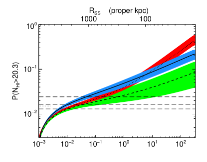
Figure 7.— Toy model prediction for the probability of a quasar at $z\sim 3.4$ with $i=19.5$ having a proximate DLA within $3000~{}~{}{\rm km~{}s}^{-1}$ as a function of volume density. The upper x-axis shows self-shielding radius, which is the minimum distance from the quasar at which a DLA can survive for a given volume density. The curves and shaded regions show the predictions and $1\sigma$ errors for the quasar-absorber correlation function $\xi_{\rm QA}$ estimated from the transverse direction in § 5, as well as the clustering strength measured by AS05. The linestyles and colors correspond to the same models as in Figure 4. The long-dashed horizontal lines indicate the measurement and $\pm 1\sigma$ range measured by Russell et al. (2006) $P_{\rm DLA}=0.013^{+0.006}_{-0.002}$ . The short dotted horizontal line is the cosmic average (i.e. no clustering) measured by (Prochaska et al. 2005). This model suggests that DLAs with volume densities in the range $10^{-2}~{}{\rm cm^{-3}}\lesssim n_{\rm H}\lesssim 10^{-1}~{}{\rm cm^{-3}}$ are required to agree with the proximate DLA measurement of Russell et al. (2006).

In this section we use a toy model to illustrate how quasar-absorber clustering can be used to constrain the physical properties of optically thick absorbers. The criteria $\delta<1$ in eqn. (10), gives a minimum distance from the quasar, $R_{\rm SS}(n_{\rm H})$ as a function of volume density, at which an optically thick absorption line system with column density $N_{\rm HI}$ can survive. Our approach is to simply assume that absorbers at smaller distances are photoevaporated and absorbers at larger distances survive. We also assume that the transverse direction is not illuminated by the quasar, and hence the transverse clustering measures the intrinsic quasar-absorber clustering, in the absence of ionization effects. Because proximate absorbers are definitely illuminated, this intrinsic clustering is then reduced along the line-of-sight by photoevaporation.

For the column density range $\log N_{\rm HI}>20.3$, we evaluate $R_{\rm SS}$ at the lower limit $\log N_{\rm HI}=20.3$, which is a decent approximation because the column density distribution is steep, and the statistics will be dominated by absorbers near the threshold. To simplify the computation, we take $R_{\rm SS}$ to be a distance only along the line of sight, which is valid provided that $R_{\rm SS}\gg\sqrt{A}$. Then we can write that the line density of absorbers within $\Delta v<3000~{}~{}{\rm km~{}s}^{-1}$ is

$$\frac{dN}{dz}=\left\langle\frac{dN}{dz}\right\rangle\left[1-\frac{aR_{\rm SS}H(z)}{\Delta v}+\chi_{\parallel}(\Delta v)\right],$$ (12)

where $\chi_{\parallel}$ is given by eqn. (5) but with $Z_{\rm cut}=R_{\rm SS}$. The assumption that the transverse direction gives the intrinsic clustering in the absence of ionization effects amounts to using the correlation function $\xi_{\rm QA}$, measured from the transverse clustering, in the line-of-sight integral in eqn. (5).

In Figure 7 we show our toy model prediction for the probability of a quasar having a proximate DLA with $\log N_{\rm HI}>20.3$ within $\Delta v<3000~{}~{}{\rm km~{}s}^{-1}$, as a function of total volume density of hydrogen $n_{\rm H}$. We assumed that the DLAs have a size of $r_{\rm abs}=5~{}h^{-1}{\rm\ kpc}$ characteristic of the ‘small’ absorbers discussed in § 6. However, identical results are obtained for ‘large’ absorbers ($r_{\rm abs}=20~{}h^{-1}{\rm\ kpc}$). Because our toy model excludes small scales $r_{\rm abs}\ll R_{\rm SS}$ from the clustering integral in eqn. (5), we are again in the far-field limit where the the volume average is nearly independent of the absorber cross section. This independence breaks down for very large densities $n_{\rm H}\gtrsim 10^{2}$, where $R_{\rm SS}$ approaches the size of the absorbers (see Figure 7). The curves and shaded regions show the predictions and $1\sigma$ errors for the transverse clustering measured in § 5, as well as the clustering strength measured by AS05. We assumed a quasar with magnitude $i=19.5$ at $z=3.335$, chosen to match the mean magnitude and redshift of the proximate DLA sample of Russell et al. (2006). The long-dashed horizontal lines indicate the measurement and $\pm 1\sigma$ range measured by Russell et al. (2006), $P_{\rm DLA}=0.013^{+0.006}_{-0.002}$ .

Our toy model suggests that DLAs with volume densities in the range $10^{-2}~{}{\rm cm^{-3}}\lesssim n_{\rm H}\lesssim 10^{-1}~{}{\rm cm^{-3}}$ are required to agree with the measurement of Russell et al. (2006). Even the weaker AS05 clustering of LBGs around quasars would require $n_{\rm H}\lesssim 1~{}{\rm cm^{-3}}$. For larger volume densities, DLAs illuminated by quasars would survive at smaller radii where the clustering is strong, giving rise to a larger number of proximate DLAs. Note that the comparison of our toy model to the Russell et al. (2006) measurement in Figure 7 assumes that the clustering of absorbers is independent of column density threshold (i.e. our measurement is for $\log N_{\rm HI}>19$) and that there is negligible evolution in the clustering between the mean redshift of our clustering sample, $z=2.5$ and that of the Russell et al. (2006) sample $z=3.335$. These assumptions were made because our quasar-absorber sample did not have sufficient statistics to measure the clustering (see § 5) in the same redshift and column density range as the Russell et al. (2006) proximate DLA measurement.

Although crude, this model illustrates how a comparison of line-of-sight and transverse quasar absorber clustering can be used to determine the density distribution in optically thick absorbers. Detailed models of self-shielding with radiative transfer (Zheng & Miralda-Escudé 2002a; Cantalupo et al. 2005; Kollmeier et al. 2006) would be required for a more accurate treatment, and such analyses could easily include cuspy density profiles or a multiphase distribution of gas. Although better statistics and more theoretical work are necessary, the clustering of optically thick absorbers around quasars will provide important new constraints on the physical nature of these systems.

8. Summary and Discussion

8.1. Summary

In this paper we used a sample of 17 super-LLSs ($\log N_{\rm HI}<19$) selected from 149 projected quasar pairs sightlines in QPQ1 to investigate the clustering pattern of optically thick absorbers around quasars. Based on this data, this paper presented the following results:

1. A simple formalism was presented for quantifying the clustering of absorbers around quasars in both the transverse and line-of-sight directions. The clustering of absorbers around quasars in the transverse direction is independent of the size of the absorption cross section; whereas, the line-of-sight clustering was shown to be sensitive to the cross section size.

2. Applying this formalism to the 17 super-LLSs ($\log N_{\rm HI}<19$) selected from 149 projected quasar pair sightlines with mean redshift $z=2.5$, we determined a comoving correlation length of $r_{0}=9.2^{+1.5}_{-1.7}~{}h^{-1}{\rm\ Mpc}$ for a power law correlation function with $\gamma=1.6$. This is three times stronger than the clustering of LBGs around quasars recently measured by AS05. If we assume a steeper slope of $\gamma=2.0$, we measure $r_{0}=5.8^{+1.0}_{-0.6}~{}h^{-1}{\rm\ Mpc}$.

3. The clustering of optically thick absorbers around quasars is highly anisotropic. If we apply the clustering amplitude measured in the transverse direction to the line-of-sight, the fraction of quasars which have a proximate absorber within $\Delta v<3000~{}~{}{\rm km~{}s}^{-1}$ is overpredicted by a factor as large as $\sim 4-20$, depending on assumptions about cross section sizes and the slope of the correlation function. The most plausible explanation for the anisotropy is that the transverse direction is less likely to be illuminated by ionizing photons than the line-of-sight, and that the optically thick absorbers along the line-of-sight are being photoevaporated.

4. A simple model of absorbers as uniform spherical overdensities is discussed and we write down an analytic criterion which determines whether an absorber illuminated by a quasar will be able to self-shield. This criterion indicates that optically thick absorbers with $n_{\rm H}\lesssim 0.1$ will be photoevaporated if they lie within $\sim 1~{}{\rm Mpc}$ of a luminous quasar. We combine this criterion with a toy model of how photoevaporation affects the line-of-sight clustering, to illustrate how comparisons of the line-of-sight and transverse clustering around quasars can ultimately be used to constrain the distribution of gas in optically thick absorption line systems.

8.2. Discussion

The anisotropic clustering pattern of absorbers around quasars suggests that the transverse direction is less likely to be illuminated by ionizing photons than the line-of-sight. This suggestion gains credibility in light of the null detections of the transverse proximity effect in the Ly$\alpha$ forests of projected quasar pairs (Crotts 1989; Dobrzycki & Bechtold 1991; Fernandez-Soto, Barcons, Carballo, & Webb 1995; Liske & Williger 2001; Schirber, Miralda-Escudé, & McDonald 2004; Croft 2004, but see Jakobsen et al.2003). Although these studies are each based only on a handful of projected pairs, they all come to similar conclusions: the amount of (optically thin) Ly$\alpha$ forest absorption, in the background quasar sightline near the redshift of the foreground quasar, is larger than average rather than smaller – the opposite of what is expected from the transverse proximity effect. Two physical effects can explain both the optically thin results and our result for optically thick systems: anisotropic emission or variability, which we discuss in turn.

If quasar emission is highly anisotropic, the line-of-sight would be exposed to the ionizing flux of the quasar; whereas, transverse absorbers would be more likely to lie in shadowed regions. Studies of Type II quasars and the X-ray background suggest that quasars with luminosities comparable to our foreground quasar sample ($M_{\rm B}<-23$) have $\sim 30\%$ of the solid angle obscured (Ueda et al. 2003; Barger et al. 2005; Treister & Urry 2005), although these estimates are highly uncertain. Naively, we would expect the covering factor of transverse absorbers to be approximately equal to the average fraction of the solid angle obscured. But in QPQ1 we found a very high covering factor (6/8) for having an optically thick absorber with $\log N_{\rm HI}>17.2$ (see Figure 1 of QPQ1) on the smallest (proper) scales $R<150~{}h^{-1}{\rm\ kpc}$. Although the statistics are clearly very poor, this high covering factor is suggestive of a significantly larger obscured fraction.

If the ionizing flux of the foreground quasar varies considerably on a timescale shorter than the transverse light crossing time between the foreground and background sightlines, a transverse proximity effect might not be observable. This is because the ionization state of the gas along the transverse sightlines is sensitive to the foreground quasars luminosity a light crossing time before the light that we observe was emitted. At $60^{\prime\prime}$ ($1.2~{}h^{-1}{\rm\ Mpc}$) from a $z=2.5$ quasar the transverse light crossing time is $1.1\times 10^{6}$ yr.

Currently, the lower limit on the intermittency of quasar emission comes from observations of the (optically thin) proximity effect (Bajtlik et al. 1988; Scott et al. 2000), in the Ly$\alpha$ forests near quasars. The presence of an optically thin proximity effect implies that the IGM has had time to reach ionization equilibrium with the quasars increased ionizing flux, which requires that the duration of a burst of quasar radiation is longer than the IGM equilibration time, $t_{\rm burst}\gtrsim 10^{4}$ yr (Martini 2004). The photoevaporation timescale for an optically thick absorber is $\sim N_{\rm HI}/F$ or the light crossing time, whichever is longer, where $F$ is the ionizing flux. At a distance of $100~{}{\rm kpc}$ from an $i=19$ quasar, it would take $15,000$ yr to photoevaporate a DLA with $\log N_{\rm HI}=20.3$, i.e. comparable to the light crossing time if DLAs have sizes of $\sim 5~{}{\rm kpc}$. Thus the time it takes for the line-of-sight to manifest the effects of the quasars ionizing flux is $\sim 10^{4}~{}{\rm yr}$ for both the optically thin and optically thick regimes. Hence, if quasars emit in bursts of duration $10^{4}~{}{\rm yr}\lesssim t_{\rm burst}\lesssim 10^{6}~{}{\rm yr}$, this would suffice to explain the absence of the optically thin transverse proximity effect as well as the anisotropic clustering pattern of optically thick absorbers discovered here.

The optically thin proximity effects are probably the most promising way to disentangle whether obscuration or variability can explain why the transverse direction is less likely to be illuminated by ionizing photons (Schirber, Miralda-Escudé, & McDonald 2004; Croft 2004). This is because for the lower column density absorbers characteristic of the Ly$\alpha$ forest, cosmological N-body simulations can predict the statistical properties of the absorbers ab initio without the complications of radiative transfer.

It might seem puzzling that we measure a clustering amplitude which is a factor of three larger than the clustering of LBGs around quasars at similar redshift measured by AS05. One could argue that on small scales we are probing material intrinsic to the quasar. If interpreted as clustering, this intrinsic contribution would lead us to overestimate the correlation function. However, only our closest sightline ($R=22~{}h^{-1}{\rm\ kpc}$, proper) is sufficiently small for this to be a worry, and this would imply a very large cross section for DLA absorption. AS05 excluded small scales from their analysis, whereas, the strength of our signal is in part driven by the small scale systems. If we exclude sightlines with $R<500~{}h^{-1}{\rm\ kpc}$ we measure a $r_{0}=7.6^{+1.9}_{-2.0}h^{-1}{\rm\ Mpc}$ which is within $1\sigma$ of the AS05 measurement. It is also possible that we measured a larger clustering signal because the galaxies which host optically thick absorbers are more strongly biased with respect to the dark matter distribution than LBGs (but see Cooke et al. 2006).

We argued that the transverse clustering predicts that galaxies correlated with a quasar should give rise to an absorption line systems with $\log N_{\rm HI}>19$ within $\Delta v<3000~{}~{}{\rm km~{}s}^{-1}$ a significant fraction of the time $\sim 15-50\%$. We postulated that these systems are not observed because of photoevaporation, but shouldn’t a similar argument also apply to galaxies? High redshift galaxy spectra should show optically thick absorption due to nearby correlated galaxies, in addition to intrinsic absorption due to H I in the galaxy itself. The individual spectra of high redshift galaxies rarely have high enough signal-to-noise ratio to detect even DLAs. However, the break due to Lyman limit absorption can be detected in very deep integrations with the added advantage that the LLSs are much more abundant. Recently, Shapley et al. (2006) detected emission blueward of the Lyman limit in 2 out of 14 LBGs at $z\sim 3$. For a galaxy-absorber correlation length in the range $r_{0}=5-10~{}h^{-1}{\rm\ Mpc}$, eqn. (2) would predict that $25-75\%$ of galaxies should show a correlated absorber within a window of $\Delta v<500~{}~{}{\rm km~{}s}^{-1}$, comparable to the redshift uncertainties of LBGS. This number assumes LLSs with $\log N_{\rm HI}>17.2$ have a size of $\sim 50~{}h^{-1}{\rm\ kpc}$ and we used the abundance of LLSs measured by Péroux et al. (2003). While it is possible that the lack of flux blueward of the Lyman limit in LBGs is due to absorption by gas intrinsic to the LBG, correlated absorbers along the line of sight could also play a significant role.

Using the ionizing flux of a quasar to study the distribution of neutral gas in optically thick absorbers is a powerful new way to study these absorption line systems. We showed how comparisons of the line-of-sight and transverse clustering of absorbers around quasars constrains their distribution of gas. Theoretical models of LLSs and DLAs which include radiative transfer and self-shielding (Zheng & Miralda-Escudé 2002a; Cantalupo et al. 2005; Kollmeier et al. 2006) should explore how morphology, cuspy density profiles, or a multiphase medium, change the ability of absorbers to survive near quasars.

Optically thick H I clouds in ionization equilibrium with a radiation field, re-emit $\sim 60\%$ of the ionizing photons they absorb as fluorescent Ly$\alpha$ recombination line photons (Gould & Weinberg 1996; Zheng & Miralda-Escudé 2002b; Cantalupo et al. 2005; Adelberger et al. 2006; Kollmeier et al. 2006). Recently, Adelberger et al. (2006) reported a detection of fluorescence from a serendipitously discovered DLA ($\log N_{\rm HI}=20.4$) situated $49^{\prime\prime}$ away from a luminous quasar at $z=2.84$. Fluorescent Ly$\alpha$ emission from absorbers illuminated by quasars offers a new window to study physical properties of absorbers, as well as a second transverse sightline to observe the ionizing flux of a quasar. In QPQ1 we published seven new quasar-absorber pairs which would have fluorescent surface brightnesses of $\mu_{{\rm Ly}\alpha}=19.5-24.3~{}{\rm mag~{}arcsec}^{-2}$, if the foreground quasars emit isotropically. However, the clustering anisotropy discussed here suggests that these transverse absorbers may not be illuminated, and the lack of a detection of fluorescent emission would provide compelling evidence in favor of this conclusion. Constraints on fluorescent emission from these systems will be discussed in the next paper in this series (Hennawi & Prochaska 2006). It is particularly intriguing that proximate DLAs observed along the line-of-sight, seem to preferentially exhibit Ly$\alpha$ emission superimposed on the Ly$\alpha$ absorption trough (Møller et al. 1998; Ellison et al. 2002). Is this Ly$\alpha$ emission fluorescence? Is the fluorescent emission from proximate DLAs observable?

In QPQ1 we argued that a factor of $\sim 20$ more transverse quasar-absorber pairs could be compiled in a modest amount of observing time, which would improve our measurement of the transverse correlation function by a factor of $\sim 5$. The study of Russell et al. (2006) searched $\sim 700$ SDSS quasars for DLAs and found 12 proximate DLAs with $\Delta v<3000~{}~{}{\rm km~{}s}^{-1}$. However, the full SDSS quasar survey has $\sim 10,000$ quasars with $z\gtrsim 2.2$ (Schneider et al. 2006), which could be used to search for proximate systems and increase the number known to $\gtrsim 100$. This would be sufficient to measure the column density distribution $f(N_{N_{\rm HI}})$ of absorbers near quasars, and any differences between it and the distribution in the ‘field’ would provide an important new constraint on the physical nature of optically thick absorbers. Finally, we note that similar studies using projected quasar pairs and searching for line-of-sight proximate absorbers can be conducted for Mg II, C IV or other metal absorption lines systems near quasars (Bowen et al. 2006; Prochter, Hennawi, & Prochaska 2006), yielding similar insights into their physical nature.

Large samples of optically thick absorption line systems near quasars are well within reach, for transverse systems using quasar pairs as well as proximate absorbers along the line-of-sight. This data will provide new opportunities to characterize the environments of quasars, the physical nature of absorption line systems, and it will uncover new laboratories for studying fluorescent emission from optically thick absorbers.

References

- Adelberger et al. (2003) Adelberger, K. L., Steidel, C. C., Shapley, A. E., & Pettini, M. 2003, ApJ, 584, 45
- Adelberger et al. (2005a) Adelberger, K. L., Steidel, C. C., Pettini, M., Shapley, A. E., Reddy, N. A., & Erb, D. K. 2005, ApJ, 619, 697
- Adelberger (2005b) Adelberger, K. L. 2005, ApJ, 621, 574
- Adelberger & Steidel (2005) Adelberger, K. L., & Steidel, C. C. 2005, ApJ, 630, 50
- Adelberger et al. (2006) Adelberger, K. L., Steidel, C. C., Kollmeier, J. A., & Reddy, N. A. 2006, ApJ, 637, 74
- Alam & Miralda-Escudé (2002) Alam, S. M. K., & Miralda-Escudé, J. 2002, ApJ, 568, 576
- Bahcall & Chokshi (1991) Bahcall, N. A. & Chokshi, A. 1991, ApJ, 380, L9
- Bahcall, Schmidt, & Gunn (1969) Bahcall, J. N., Schmidt, M., & Gunn, J. E. 1969, ApJ, 157, L77
- Bajtlik et al. (1988) Bajtlik, S., Duncan, R. C., & Ostriker, J. P. 1988, ApJ, 327, 570
- Barger et al. (2005) Barger, A. J., Cowie, L. L., Mushotzky, R. F., Yang, Y., Wang, W.-H., Steffen, A. T., & Capak, P. 2005, AJ, 129, 578
- Bertoldi (1989) Bertoldi, F. 1989, ApJ, 346, 735
- Bouché & Lowenthal (2004) Bouché, N., & Lowenthal, J. D. 2004, ApJ, 609, 513
- Bowen et al. (2006) Bowen, D. V., et al. 2006, submitted
- Briggs et al. (1989) Briggs, F. H., Wolfe, A. M., Liszt, H. S., Davis, M. M., & Turner, K. L. 1989, ApJ, 341, 650
- Brown, Boyle, & Webster (2001) Brown, M. J. I., Boyle, B. J., & Webster, R. L. 2001, AJ, 122, 26
- Cantalupo et al. (2005) Cantalupo, S., Porciani, C., Lilly, S. J., & Miniati, F. 2005, ApJ, 628, 61
- Coil et al. (2005) Coil, A. L., Newman, J. A., Cooper, M. C., Davis, M., Faber, S. M., Koo, D. C., & Willmer, C. N. A. 2005, ArXiv Astrophysics e-prints, arXiv:astro-ph/0512233
- Coil et al. (2006) Coil, A. L., et al. 2006, submitted
- Conroy et al. (2005) Conroy, C., Wechsler, R. H., & Kravtsov, A. V. 2005, ArXiv Astrophysics e-prints, arXiv:astro-ph/0512234
- Cooke et al. (2006) Cooke, J., Wolfe, A. M., Gawiser, E., & Prochaska, J. X. 2006, ApJ, 636, L9
- Croft (2004) Croft, R. A. C. 2004, ApJ, 610, 642
- Croom et al. (2004) Croom, S. M., Smith, R. J., Boyle, B. J., Shanks, T., Miller, L., Outram, P. J., & Loaring, N. S. 2004, MNRAS, 349, 1397
- Crotts (1989) Crotts, A. P. S. 1989, ApJ, 336, 550
- Dobrzycki & Bechtold (1991) Dobrzycki, A. & Bechtold, J. 1991, ApJ, 377, L69
- Ellison et al. (2002) Ellison, S. L., Yan, L., Hook, I. M., Pettini, M., Wall, J. V., & Shaver, P. 2002, A&A, 383, 91
- Ferland et al. (1998) Ferland, G. J., Korista, K. T., Verner, D. A., Ferguson, J. W., Kingdon, J. B., & Verner, E. M. 1998, PASP, 110, 761
- Fernandez-Soto, Barcons, Carballo, & Webb (1995) Fernandez-Soto, A., Barcons, X., Carballo, R., & Webb, J. K. 1995, MNRAS, 277, 235
- Gawiser et al. (2001) Gawiser, E., Wolfe, A. M., Prochaska, J. X., Lanzetta, K. M., Yahata, N., & Quirrenbach, A. 2001, ApJ, 562, 628
- Gould & Weinberg (1996) Gould, A., & Weinberg, D. H. 1996, ApJ, 468, 462
- Haardt & Madau (1996) Haardt, F.,& Madau, P. 1996,ApJ, 461, 20
- Hennawi et al. (2006a) Hennawi, J. F., et al. 2006, AJ, 131, 1
- Hennawi et al. (2006) Hennawi, J. F., et al. 2006, ArXiv Astrophysics e-prints, arXiv:astro-ph/0603742
- Hennawi & Prochaska (2006) Hennawi, J. F. & Prochaska, J. X. 2006, in preparation
- Jakobsen et al. (2003) Jakobsen, P., Jansen, R. A., Wagner, S., & Reimers, D. 2003, A&A, 397, 891
- Kollmeier et al. (2006) Kollmeier, J. A., et al., in preparation
- Lee et al. (2006) Lee, K.-S., Giavalisco, M., Gnedin, O. Y., Somerville, R. S., Ferguson, H. C., Dickinson, M., & Ouchi, M. 2006, ApJ, 642, 63
- Liske & Williger (2001) Liske, J., & Williger, G. M. 2001, MNRAS, 328, 653
- Lopez et al. (2005) Lopez, S., Reimers, D., Gregg, M. D., Wisotzki, L., Wucknitz, O., & Guzman, A. 2005, ApJ, 626, 767
- Martini (2004) Martini, P. 2004, Coevolution of Black Holes and Galaxies, 169
- Meiksin (2005) Meiksin, A. 2005, MNRAS, 356, 596
- Miralda-Escudé (2003) Miralda-Escudé, J. 2003, ApJ, 597, 66
- Møller et al. (1998) Moller, P., Warren, S. J., & Fynbo, J. U. 1998, A&A, 330, 19
- Møller et al. (2002) Møller, P., Warren, S. J., Fall, S. M., Fynbo, J. U., & Jakobsen, P. 2002, ApJ, 574, 51
- O’Meara et al. (2006) O’Meara, J. M., et al. 2006, in preparation
- Oort & Spitzer (1955) Oort, J. H., & Spitzer, L. J. 1955, ApJ, 121, 6
- Ouchi et al. (2005) Ouchi, M., et al. 2005, ApJ, 635, L117
- Péroux et al. (2003) Péroux, C., McMahon, R. G., Storrie-Lombardi, L. J., & Irwin, M. J. 2003, MNRAS, 346, 1103
- Péroux et al. (2005) Péroux, C., Dessauges-Zavadsky, M., D’Odorico, S., Sun Kim, T., & McMahon, R. G. 2005, MNRAS, 363, 479
- Prochaska (1999) Prochaska, J. X. 1999, ApJ, 511, L71
- Prochaska et al. (2005) Prochaska, J. X., Herbert-Fort, S., & Wolfe, A. M. 2005, ApJ, 635, 123
- Prochaska & Hennawi (2006) Prochaska, J. X., & Hennawi, J. F. 2006, in preparation
- Prochter, Hennawi, & Prochaska (2006) Prochter, G. E., Hennawi,J. F., & Prochaska, J. X. 2006, in preparation
- Richards et al. (2002) Richards, G. T., Vanden Berk, D. E., Reichard, T. A., Hall, P. B., Schneider, D. P., SubbaRao, M., Thakar, A. R., & York, D. G. 2002, AJ, 124, 1
- Russell et al. (2006) Russell, D. M., Ellison, S. L., & Benn, C. R. 2006, MNRAS, 367, 412
- Schaye (2001) Schaye, J. 2001, ApJ, 559, 507
- Schirber, Miralda-Escudé, & McDonald (2004) Schirber, M., Miralda-Escudé, J., & McDonald, P. 2004, ApJ, 610, 105
- Schneider et al. (2006) Schneider, D. P., et al. 2006, in preparation
- Scott et al. (2000) Scott, J., Bechtold, J., Dobrzycki, A., & Kulkarni, V. P. 2000, ApJS, 130, 67
- Serber et al. (2006) Serber, W., et al.2005, about to be submitted.
- Shapley et al. (2006) Shapley, A. E., et al. 2006, submitted
- Smette et al. (1995) Smette, A., Robertson, J. G., Shaver, P. A., Reimers, D., Wisotzki, L., & Koehler, T. 1995, A&AS, 113, 199
- Smith, Boyle, & Maddox (2000) Smith, R. J., Boyle, B. J., & Maddox, S. J. 2000, MNRAS, 313, 252
- Spergel et al. (2003) Spergel, D. N., et al. 2003, ApJS, 148, 175
- Spitzer (1978) Spitzer, L. 1978, New York Wiley-Interscience, 1978. 333 p., 246
- Treister & Urry (2005) Treister, E., & Urry, C. M. 2005, ApJ, 630, 115
- Ueda et al. (2003) Ueda, Y., Akiyama, M., Ohta, K., & Miyaji, T. 2003, ApJ, 598, 886
- Yee & Green (1984) Yee, H. K. C. & Green, R. F. 1984, ApJ, 280, 79
- Yee & Green (1987) Yee, H. K. C. & Green, R. F. 1987, ApJ, 319, 28
- Zheng & Miralda-Escudé (2002a) Zheng, Z., & Miralda-Escudé, J. 2002, ApJ, 568, L71
- Zheng & Miralda-Escudé (2002b) Zheng, Z., & Miralda-Escudé, J. 2002, ApJ, 578, 33