Influence of Thermalisation on Electron Injection
in Supernova Remnant Shocks
O. Petruk¹ and R. Bandiera^2
1Institute for Applied Problems in Mechanics and Mathematics,
Naukova St. 3-b, Lviv 79000, Ukraine
petruk@astro.franko.lviv.ua
²Osservatorio Astrofisico di Arcetri,
Largo E.Fermi 5, Firenze 50125, Italy
bandiera@arcetri.astro.it

Abstract. Within a test-particle description of the acceleration process in parallel nonrelativistic shocks, we present an analytic treatment of the electron injection. We estimate the velocity distribution of the injected electrons as the product of the post-shock thermal distribution of electrons times the probability for electrons with a given velocity to be accelerated; the injection efficiency is then evaluated as the integral of this velocity distribution. We estimate the probability of a particle to be injected as that of going back to the upstream region at least once. This is the product of the probability of returning to the shock from downstream times that of recrossing the shock from downstream to upstream. The latter probability is expected to be sensitive to details of the process of electron thermalisation within the (collisionless) shock, a process that is poorly known. In order to include this effect, for our treatment we use results of a numerical, fully kinetic study, by Bykov & Uvarov (1999). According to them, the probability of recrossing depends on physics of thermalisation through a single free parameter ($\Gamma$), which can be expressed as a function of the Mach number of the shock, of the level of electron-ion equilibration, as well as of the spectrum of turbulence. It becomes apparent, from our analysis, that the injection efficiency is related to the post-shock electron temperature, and that it results from the balance between two competing effects: the higher the electron temperature, the higher the fraction of downstream electrons with enough velocity to return to the shock and thus to be ready to cross the shock from downstream to upstream; at the same time, however, the higher the turbulence, which would hinder the crossing.

Keywords: Shock waves, acceleration of particles, cosmic rays, supernova remnants

PACS numbers: 98.38.Mz, 95.30.Lz

1 Introduction

Strong collisionless shocks are present in various astrophysical objects, and under a wide range of conditions. These shocks effectively heat the gas and are also believed to accelerate a fraction of particles up to very high energies. Analyses based on multi-frequency observations allow one to determine properties of both thermal and nonthermal component. In the case of supernova remnants (hereafter SNRs), optical and UV emission are typically thermal, radio is nonthermal, while thermal and nonthermal emission may coexist in X-rays. The momentum distribution of the accelerated particles is locally well approximated by a power law; this can be inferred from the power-law synchrotron spectra, in the case of electrons; while in the case of ions it can be measured directly in the energy distribution of cosmic rays (if one accepts the ‘‘SNR Paradigm’’ for the origin of galactic cosmic rays).

Diffusive acceleration (Fermi acceleration) is believed to be the dominant process that allows particles to gain energies in excess of typically thermal values. The standard theory of diffusive acceleration, in test-particle approximation (see e.g. the review of Jones & Ellison [12]), shows that a power-law distribution develops at high energies. The spectral index of this high-energy population depends on the shock compression ratio, while it does not depend at all on the original energy distribution of the injected particles. In fact, a simplified way to describe the overall particle evolution, from nearly thermal to very high velocities, is to treat particle injection and acceleration as two separate problems. The injection problem consists in finding out the initial momentum distribution of that fraction of (originally thermal) particles that can enter the acceleration process, i.e. to make at least one acceleration cycle. The acceleration problem, instead, consists in following the evolution of the distribution of these particles along all next acceleration cycles.

In order to keep the number of free parameters low, while modelling more effectively the emission in all observed spectral ranges, one needs to introduce a physically self-consistent scenario for the thermal and nonthermal populations. For instance, the standard model of particle acceleration constrains the slope of the electron distribution at high velocities, but does not predict its normalization: in other terms, the injection efficiency (i.e. the fraction of particles that enter the acceleration process) is poorly known, because this process is sensitive to physical details not included in the standard model of Fermi acceleration. The level of electron-ion equilibration or, alternatively, the electron temperature is another key quantity hard to determine ‘‘a priori’’ in collisionless shocks. While in models of SNR shocks injection and equilibration efficiencies are taken as independent free parameters, in the reality both depend on the physical conditions within the shock transition, and therefore they are not independent. Goal of this paper is in fact to investigate, in nonrelativistic SNR shocks, a possible connection between electron injection and thermal equilibration.

A self-consistent treatment of injection and acceleration must include a microphysical model of particle-wave interactions in the plasma. A few physical processes have been proposed to account for the electron injection (see Malkov & Drury [19] for a review). The scattering of electrons is suggested to be due to some ion-generated instabilities (Bykov & Uvarov [4]; hereafter BU99), whistler waves [17] and lower-hybrid waves from ions [16]. These models mainly address the plasma microphysics; while only BU99, to our knowledge, are able to model the formation of the post-shock electron distribution.

In this paper, we approach the problem in a simplified way. We assume the presence of scattering centres, without concentrating on their nature, but simply assuming that they match the following requirements: i) the interaction with these scattering centres generates a nearly isotropic, Maxwellian velocity distribution of particles on timescales not longer than one collision time; ii) the timescales for (wave-mediated) isotropization and energy exchange between electrons are both smaller than the (wave-mediated) electron-ion equilibration time; iii) the scattering centres play at the same time the role of thermalising, within the shock, the incoming particle population to the post-shock temperature and that of driving the process of diffusive acceleration. When we will need to use more specific properties of the wave-particle interaction (in Sect. 3.2), we will refer to the results of BU99 on the electron kinetics.

There are in general three ways to calculate the post-shock momentum distribution of particles: either by solving the kinetic equations, or by making a hybrid simulation (which is however unable to model the momentum distribution of electrons because electrons are treated as a fluid), or finally by extending the individual particle approach of Bell [1]. He has estimated the probability for a particle to return to the shock from downstream and has shown that in this way one obtains a power-law distribution for the accelerated particles with velocities $v\gg V_{\mathrm{s}}$ (where $V_{\mathrm{s}}$ is the shock velocity).

In the present paper we propose to extend the Bell approach to the problem of injection by introducing the probability to recross the shock from downstream to upstream. This probability is connected to the process of thermalisation of the incoming flow within the shock. This fact has been shown by Malkov [18] in the case of protons. Namely, the idea that ions are prevented from backstreaming by the self-generated waves (which also participate in thermalisation of ions) has allowed Malkov to obtain an analytic solution of the injection problem for protons. The main point in his thermal leakage theory is that only those protons that can ‘‘leak’’ upstream are injected into the Fermi process.

We use the same idea in our approach to electrons, even though we are not tight to any specific kind of interaction. We consider only the case of parallel shocks, namely when the ambient magnetic field is parallel to the shock normal.

The plan of the present paper is as follows. In Sect. 2 we deal with the injection problem by developing an analytic treatment for calculating the injection efficiency as well as for determining of the distribution of particles which are able to be accelerated. Sect. 3 deals with the process of thermalisation and its influence on injection and, using results from BU99 model, give quantitative estimations on the injection efficiency. Sect. 4 concludes.

2 Injection efficiency and initial distribution

2.1 Efficiency of electron injection

Let us assume that all electrons are injected into the acceleration process from the downstream thermal population, i.e. we do not invoke seed particles with velocities already much higher than the thermal velocity. Their distribution is then well approximated by $n_{\mathrm{es}}f_{\mathrm{M}}$, where

$$f_{\mathrm{M}}(y)={4\over\sqrt{\pi}}y^{2}\exp(-y^{2})$$ (1)

is a normalized Maxwellian, isotropic in the fluid comoving frame. We have introduced the reduced momentum $y=p/p_{\mathrm{th}}$, which is also equal to the reduced velocity $v/v_{\mathrm{th}}$, as long as non-relativistic particles are considered, as it is the case at injection. Thermal momentum and velocity are defined by $p_{\mathrm{th}}=m_{\mathrm{e}}v_{\mathrm{th}}=\sqrt{2m_{\mathrm{e}}kT_{\mathrm{es}}}$, where $T_{\mathrm{es}}$ is the post-shock electron temperature. We consider a fully ionized H+He gas (with $n_{\mathrm{He}}=0.1n_{\mathrm{H}}$, for a mean mass per particle $\mu=0.609$), and a strong, unmodified shock. For an adiabatic index $\gamma=5/3$, the shock compression ratio is $\sigma=4$ but, for the sake of generality, in the following formulae we shall allow for a general $\sigma$. Therefore, the ratio of the electron thermal velocity, $v_{\mathrm{th}}$, to $V_{\mathrm{s}}$ is

$${v_{\mathrm{th}}\over V_{\mathrm{s}}}=\sqrt{{2(\sigma-1)\over\sigma^{2}}{\chi_{\mathrm{s}}\over\chi_{\mathrm{o}}}},$$ (2)

where $\chi_{\mathrm{o}}=m_{\mathrm{e}}/(\mu m_{\mathrm{p}})\simeq 8.94\times 10^{-4}$. The factor $\chi_{\mathrm{s}}=T_{\mathrm{es}}/T_{\mathrm{s}}$, where $T_{\mathrm{s}}$ is the mean shock temperature, accounts for the thermal equilibration level between electrons and ions immediately after the shock, and ranges from $\chi_{\mathrm{o}}$ (no equilibration) to 1 (full equilibration).

Introducing the simple-minded assumption that only particles in the high-velocity tail of the Maxwellian distribution can be accelerated, it is easy to link the minimum momentum of this tail, $p_{\mathrm{tail}}=y_{\mathrm{tail}}p_{\mathrm{th}}$, to the injection efficiency $\varsigma$ (i.e. the fraction of accelerated particles). One has just to solve the equation $\int_{y_{\mathrm{tail}}}^{\infty}f_{\mathrm{M}}(y)=\varsigma$, which gives for instance $y_{\mathrm{tail}}=2.85$ for $\varsigma=10^{-3}$ and $y_{\mathrm{tail}}=3.91$ for $\varsigma=10^{-6}$. It is worth noticing that, for reasonable values of $\varsigma$, this integral is dominated by particles with $y\sim y_{\mathrm{tail}}$, with $y_{\mathrm{tail}}$ of order of unity: it is apparent from this example that injection involves mostly particles with velocities of the order of the thermal one, and not only those with $v\gg V_{\mathrm{s}}$.

In the above estimation, we have assumed that all particles with $y>y_{\mathrm{tail}}$, and only them, are accelerated. In order to find out the injection efficiency in a more general case, we introduce the probability ${\cal P}(y)$ for a particle with velocity $v=yv_{\mathrm{th}}$ to be accelerated, i.e. to recross the shock from downstream to upstream at least once. This probability yields the fraction of particles, with a given velocity, which can be accelerated; while the Maxwellian distribution in turn gives the number density of particles with that velocity. Thus, for an isotropic velocity distribution, the fraction of accelerated particles (injection efficiency) is given by the integral

$$\varsigma=\int\limits_{0}^{\infty}{\cal P}(y)f_{\mathrm{M}}(y)\,dy.$$ (3)

In other terms, the distribution of particles injected into the acceleration process is

$$f_{\mathrm{inj}}(y)={\cal P}(y)f_{\mathrm{M}}(y).$$ (4)

The probability ${\cal P}(y)$ in turn can be estimated as the product of the probability, $P_{\mathrm{r}}$, that a particle returns to the shock from downstream, times the probability, $P_{\mathrm{c}}$, that this particle crosses the shock moving upstream. The next two subsections will be devoted to estimate these two probabilities.

We wish to point out that a common misconception lies underneath the Fermi acceleration approach, namely that the electrons must enter this process having already a velocity much higher than $V_{\mathrm{s}}$. This is usually obtained, by requiring either i) that the electron temperature is close to equipartition, or ii) that only electrons in the high-energy tail of the Maxwellian distribution enter into the acceleration process, or finally iii) that some unknown pre-acceleration mechanism takes place to accelerate electrons to the required velocity regime. The condition $v\gg V_{\mathrm{s}}$ is in fact very useful to simplify the mathematical treatment of the process, but in our belief is not strictly required by physical arguments. In the present paper we will show instead i) that electrons may be injected efficiently also when their temperatures is far from equipartition, ii) that, in order to have reasonably high injection efficiencies, $\chi_{\mathrm{s}}$ has to be considerably less than unity; in other words, the velocities of the majority of the injected electrons must not be not too far from the thermal velocity and the minimum injection momentum can even be much smaller than thermal one, and finally iii) that there is no physical need for an independent pre-acceleration process, if the treatment of the acceleration is modified in order to account also for relatively low particle velocities (this can be done by introducing the probability of crossing the shock, Sect. 2.3).

2.2 Probability of returning to the shock

In the case of isotropic velocity distribution in the downstream flow, the probability for particles with velocity $v$ to return to the shock from downstream is given by the ratio of the upstream and downstream fluxes [12]:

$$P_{\mathrm{r}}(v)={\left|\int\limits_{-v}^{-u_{2}}(u_{2}+v_{x})\,dv_{x}\right|\over\int\limits_{-u_{2}}^{v}(u_{2}+v_{x})\,dv_{x}}=\mathrm{H}(v-u_{2})\left({1-u_{2}/v\over 1+u_{2}/v}\right)^{2},$$ (5)

where: $u_{2}=V_{\mathrm{s}}/\sigma$ is the velocity of the downstream flow, in the shock reference frame; $v$ is the velocity, in the downstream flow reference frame, of the particle that has just reached the shock; $\mathrm{H}(v-u_{2})$ is the Heaviside step function (meaning that $u_{2}$ is the minimum value of $v$ that allows a particle to return to the shock). In general, in the paper we label quantities refering to upstream with ‘‘1’’ and quantities refering to downstream with ‘‘2’’. Coordinates are defined in such a way that, in the reference frame of the shock, the flow moves along the $x$-axis in the positive direction.

It is useful to re-write Eq. (2) to fix a lower boundary to the reduced momenta of the injected particles

$$y_{\mathrm{min}}={u_{2}\over v_{\mathrm{th}}}=\left({\chi_{\mathrm{o}}\over 2(\sigma-1)\chi_{\mathrm{s}}}\right)^{1/2}.$$ (6)

The quantity $y_{\mathrm{min}}$ is always less than $(2(\sigma-1))^{-1/2}$ (i.e. $p_{\mathrm{min}}<0.4p_{\mathrm{th}}$ for $\sigma=4$) and can be much smaller than that if $\chi_{\mathrm{s}}\sim 1$ (which means $v_{\mathrm{th}}\gg V_{\mathrm{s}}$). This means that, the higher the level of electron-ion equilibration, the higher the electron thermal velocity compared to $V_{\mathrm{s}}$, and thus the higher the fraction of electrons able to return to the shock from downstream.

2.3 Probability of crossing the shock

The standard theory of diffusive acceleration [1] implicitely assumes $P_{\mathrm{c}}\simeq 1$, which means that the particle mean free path $\lambda$ is longer than the thickness, $\Delta x$, of the shock transition region. This condition applies only for particles with high enough velocity ($v\gg V_{\mathrm{s}}$).

On the contrary, the evolution of particles with lower velocities is affected by scatterings within the shock transition. In fact, the mere existence of a shock implies that the incoming ambient plasma must be thermalised, within the shock transition region, by some kind of scatterings centres. Also particles that enter the shock transition region from downstream, as long as they have velocities similar to thermal particles, must experience a similar rate of scatterings. Thus, also for them $\lambda<\Delta x$.

In the presence of scatterings, only a fraction of these particles will succeed crossing the shock and finally reaching the upstream region. In general, modelling this process is very complex. Here we will present a simplified treatment, based on some approximations. The first of them is diffusive approximation, which requires that mean free paths are smaller than the shock thickness, and that the velocity distribution is nearly isotropic.

However, this assumption is invalid near the downstream boundary of the shock layer. In fact, the original distribution of downstream particles which return to the shock is highly anisotropic, since all particles entering the shock have, in the shock reference frame, an $x$-component opposite to the flow velocity. The above assumption is anyway valid over most of the volume, provided that isotropization processes within the shock are very efficient. Namely, we require that the length scale for isotropization is of the order of one mean free path (similarly to what happens for Coulomb collisions between similar particles).

The estimation of $P_{\mathrm{c}}(v)$ is generally very complex. Here we use a crude approximation (based on the so-called ‘‘modulation’’ equation, see e.g. [12]) and write

$$P_{\mathrm{c}}=\exp(-\langle u\rangle\Delta x/\kappa).$$ (7)

where $\langle u\rangle\approx(u_{1}+u_{2})/2=u_{2}(\sigma+1)/2$ and $\kappa$ is the diffusion coefficient.

We want to point out that probability of crossing is closely related to the thermalization level $\chi_{\mathrm{s}}$. The thickness $\Delta x$ may be derived from the condition that the temperature of the incoming fluid increases to the post-shock value $T_{\mathrm{es}}=\chi_{\mathrm{s}}T_{\mathrm{s}}$ while the fluid moves through the shock transition from upstream to downstream. In this way, the two problems – injection and thermalisation – become closely connected. This can be seen by rewriting

$$\Delta x=\langle u\rangle\Delta t_{12}=\langle u\rangle\int\limits_{0}^{\chi_{\mathrm{s}}}\left(\frac{d\chi}{dt}\right)^{-1}d\chi$$ (8)

where $\Delta t_{12}$ is the time it takes to a fluid element to cross the shock, moving from its upstream boundary to the downstream one. In general, it is necessary to introduce a microphysical model of thermalisation in order to obtain explicitely the functional dependence of the rate of thermalization $d\chi/dt$.

For the diffusion coefficient we use the standard formula $\kappa=\lambda^{\prime}v^{\prime}/3$, where $v^{\prime}$ is the velocity of a particle in the local reference frame of the flow and $\lambda^{\prime}$ is the particle mean free path with respect to scatterings within the shock transition. A further assumption behind this formula is that the scattering centres are frozen into the fluid. This is, for instance, the case in the BU99 model for the electron kinetics in a strong shock. In this model, particles are scattered by the ion-generated Alfvénic waves, and the Alfvénic speed is much lower than the shock velocity. In case of electron diffusion in presence of magnetic field turbulence, it is common to parametrize the mean free path as $\lambda^{\prime}=\eta r_{\mathrm{g}}$, where $r_{\mathrm{g}}=p^{\prime}c/eB$ is the gyroradius and $\eta$ accounts for the level of turbulence. We concentrate here on particles with velocities not much larger than $V_{\mathrm{s}}$, and therefore we will use the nonrelativistic formula for $\lambda^{\prime}$. For such parameterization of the mean free path, $\lambda^{\prime}$ may be written as $\lambda^{\prime}=\tau_{\mathrm{D}}v^{\prime}$ where $\tau_{\mathrm{D}}$ is the average deflection time defined as $\tau_{\mathrm{D}}=\eta m_{\mathrm{e}}c(eB)^{-1}$.

In order to compute a probability $P_{\mathrm{c}}(v)$ for particles having a given velocity $v$ in the downstream reference frame, we need to average over all $v^{\prime}$ velocities corresponding to a a given $v$ downstream. In the reference frame of the average flow within the shock transition, velocities $v^{\prime}$ corresponding to the same $v$ are different in different directions, namely $\vec{v^{\prime}}=\vec{v}-(\vec{\langle u\rangle}-\vec{u_{2}})$. The angle-averaged value of $\overline{v^{\prime 2}}$ for these particles is given by

$$\overline{v^{\prime 2}} = {\int\limits_{-v}^{-u_{2}}\left((v_{x}-u_{2}(\sigma-1)/2)^{2}+v_{\perp}^{2}\right)dv_{x}\bigg{/}\int\limits_{-v}^{-u_{2}}dv_{x}}$$ (9)

$$= v^{2}+{\sigma-1\over 2}vu_{2}+{\sigma^{2}-1\over 4}u_{2}^{2}.$$

Let us assume that, on the average, electrons in the incoming flow are thermalised to the level $\chi_{\mathrm{s}}$ in $N_{\mathrm{c}}$ collisionless interactions. For the sake of illustration, let us calculate the number of scatterings, $N_{\mathrm{c}}$, which yield a given injection efficiency. The involved time is approximately $\Delta t_{12}=N_{\mathrm{c}}\tau_{\mathrm{D}}$ and therefore

$${\langle u\rangle\Delta x\over\kappa}={3\langle u\rangle^{2}\over v^{\prime 2}}{\Delta t_{12}\over\tau_{\mathrm{D}}}={3\langle u\rangle^{2}\over v^{\prime 2}}N_{\mathrm{c}},$$ (10)

so that the probability (7) becomes

$$P_{\mathrm{c}}(v^{\prime})=\exp\left(-{3(\sigma+1)^{2}\over 4}\left({u_{2}\over v^{\prime}}\right)^{2}N_{\mathrm{c}}\right).$$ (11)

Eq. (3), together with probabilities (5), (11) and Eqs.(6), (9), shows that, in order to get an injection efficiency $\varsigma=10^{-3}$, $N_{\mathrm{c}}$ must be equal to 9 for $\chi_{\mathrm{s}}=0.001$, and to 770 for $\chi_{\mathrm{s}}=0.1$.

It is interesting to note that our expression for $P_{\mathrm{c}}$ behaves like the ‘‘leakage probability’’ $\nu_{\mathrm{esc}}$ of Malkov [18], calculated for protons. Namely, the probability for protons to leak across the shock from downstream is approximately $\nu_{\mathrm{esc}}(y)\propto\exp\left(-{\rm const}\ \left(y^{\prime}\right)^{-2}\right)$ [7].

Finally, we want to stress that the introduction of the probability $P_{\mathrm{c}}$ does not affect the slope of the accelerated spectrum at relativistic energies. Following standard test-particle approach to Fermi acceleration [1], a power-law momentum distribution of relativistic particles is generated, with an index $\alpha=-(2-\sigma)/(\sigma-1)$ that depends only on the shock compression ratio. This index is obtained by combining the term for the momentum increment per cycle ($\Delta p/p$) with that for the difference $(1-P_{\mathrm{r}})$ per cycle, in the high-velocity limit. The asymptotic behaviour of both terms is $\propto v^{-1}$; while Eq. (7) is such that $(1-P_{\mathrm{c}})\propto v^{-2}$. Therefore, in the high velocity limit $P_{\mathrm{c}}$ gives negligible contribution to the formation of the particle spectrum in comparison to $P_{\mathrm{r}}$, and does not affect the formula for $\alpha$.

3 Thermalisation of electrons and injection

In the shock-front reference frame, if upstream electrons and ions enter the leading edge of the shock transition with the same velocity then the electron energy is lower than that of protons by a factor $m_{\mathrm{e}}/m_{\mathrm{p}}$. Therefore, if the velocities of electrons and ions are randomized independently within the shock front, we obtain $T_{\mathrm{es}}=(m_{\mathrm{e}}/\mu m_{\mathrm{p}})T_{\mathrm{s}}\ll T_{\mathrm{s}}$ (i.e. $\chi_{\mathrm{s}}=\chi_{\mathrm{o}}\ll 1$ in our notation), while the ionic temperatures are about $(n_{\mathrm{e}}+n_{\mathrm{i}})T_{\mathrm{s}}/n_{\mathrm{i}}$ (where ‘‘i’’ denotes ions), namely much closer to $T_{\mathrm{s}}$.

The temperatures of electrons and ions may get closer, if there is a process within the shock which allows energy exchanges between the two species. In collisional shocks, the equilibration process is Coulomb scattering between ions and electrons, while, in the collisionless case (like it generally occurs in SNRs), turbulence plays the dominant role.

3.1 Results from observations

Since longtime, it has been suggested that plasma instabilities could lead to prominent heating of electrons within the shock (e.g.[20]). Some observations and theoretical results put forward the possibility that collisionless processes within the shock of SNRs could heat electrons up to the level $\chi_{\mathrm{s}}\simeq 0.4$ ([2] and references therein). Results on SNR DEM L71 in LMC [24] and on RCW86 [8] also suggest $\chi_{\mathrm{s}}\sim 0.3$. Analysis of Chandra data on Tycho SNR indicates that $\chi_{\mathrm{s}}\leq 0.1$ [11, 8]. Other recent observations (SN1006, Tycho, 1E 0102.2–7219) favour a considerably lower thermalisation level, namely $\chi_{\mathrm{s}}\leq 0.03\div 0.07$ [13, 26, 9, 14, 10, 15]).

It is important to know how does the level $\chi_{\mathrm{s}}$ depend on the properties of the shock. Observational estimations of the shocks with Mach number ${\cal M}$ up to $\sim 400$ suggest that stronger shocks (namely with higher $V_{\mathrm{s}}$) could equilibrate species less effectively. Namely, Schwartz et al. ([25]) present results of measurements of $T_{\mathrm{es}}/T_{\mathrm{s}}$ for interplanetary shocks and planetary bow shocks (${\cal M}\leq 25$) and find strong evidence that this ratio depends on the Mach number as ${\cal M}^{-1}$. Ghavamian et al. [8] estimations for a number of SNRs seem to extend this trend to stronger shocks, with $25\leq{\cal M}\leq 200$. Rakowski [23] summarises the observational methods and estimations of $\chi_{\mathrm{s}}$ in SNRs shocks and confirms the inverse dependence in the range $25\leq{\cal M}\leq 400$.

3.2 Results from Bykov and Uvarov (1999)

Interactions of electrons with ion- or self-generated waves could be responsible for both accelerating and heating of electrons (see [19, 3] for a review).

BU99 have considered the interactions of electrons with ion-generated electro-magnetic fluctuations and have developed a kinetic model that accounts at the same time for electron injection, acceleration and thermalisation in quasiparallel shocks. Their model is applicable for shocks with local Mach number ${\cal M}$ less than $\sim\sqrt{m_{\mathrm{p}}/m_{\mathrm{e}}}$. They have introduced the effective electron temperature $T_{\mathrm{eff}}$ (measured in units of the upstream temperature $T_{\mathrm{o}}$), which may be related to our $\chi_{\mathrm{s}}$ by

$$\chi_{\mathrm{s}}=T_{\mathrm{eff}}{T_{\mathrm{o}}\over T_{\mathrm{s}}}=T_{\mathrm{eff}}{\sigma^{2}\over(\sigma+1){\cal M}^{2}},$$ (12)

and have shown that it depends on the Mach number. This dependence can be approximately described by a power law: $T_{\mathrm{eff}}\propto{\cal M}^{a}$, with index $0<a\leq 2$ depending on which model of wave-particle interaction is considered. Therefore, the level of thermalisation depends on the velocity of the shock: $\chi_{\mathrm{s}}\propto{\cal M}^{a-2}$ for strong shocks, namely the higher the velocity the smaller the thermalisation level.

Figure 1: Injection efficiency $\varsigma$ versus post-shock ratio $\chi_{\mathrm{s}}$ for a model of BU99 for Bohm-like diffusion and diffusion boundary conditions. Curves are labelled by their respective Mach number. The approximation $\varsigma=2\times 10^{5}\left({\cal M}^{2}\chi_{\mathrm{s}}\right)^{-5}$ is shown by dashed lines.

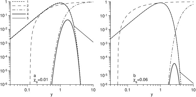
Figure 2: Electron distribution functions and probabilities calculated for two different values of $\chi_{\mathrm{s}}$. 1 – Maxwellian distribution, 2 – probability to return to the shock $P_{\mathrm{r}}$, 3 – probability to cross the shock $P_{\mathrm{c}}$, 4 – initial distribution $f_{\mathrm{inj}}$ of electrons injected into acceleration process, 5 – final hybrid electron distribution ($\alpha=2$). Plots are calculated for the model of electron-wave interaction developed by BU99 (case of Bohm-like diffusion with diffusive boundary conditions), ${\cal M}=40$. a) $\chi_{\mathrm{s}}=0.01$, in this case $y_{\mathrm{min}}=0.12$, $y_{\mathrm{b}}=2.6$, $\varsigma=0.048$, $N_{\mathrm{c}}=20$; b) $\chi_{\mathrm{s}}=0.06$, in this case $y_{\mathrm{min}}=0.05$, $y_{\mathrm{b}}=3.9$, $\varsigma=3.1\times 10^{-5}$, $N_{\mathrm{c}}=930$.

If $\lambda^{\prime}$ is momentum independent (transport of electrons is due to large-scale magnetic field fluctuations that provide effective heating) then $a\approx 2$, and the level of equilibration $\chi_{\mathrm{s}}$ does not depend on the Mach number. This means that $T_{\mathrm{es}}\propto V_{\mathrm{s}}^{2}$, but with a factor that may be higher than that inferred from Rankine-Hugoniot equations for the electron population [21]. The opposite case is when electron heating in the shock transition region is effectively suppressed by a developed small-scale vortex turbulence, giving $a\approx 0$. In such a situation the postshock electron temperature is $T_{\mathrm{es}}\approx T_{\mathrm{o}}$, independently of the Mach number. Another interesting model of wave-particle interactions is Bohm-like diffusion, for which $\lambda^{\prime}\propto p$ and $a=1$. In the present paper we consider only the Bohm-like diffusion case since it seems to be in agreement with observations (namely $\chi_{\mathrm{s}}\propto{\cal M}^{-1}$, see Sect. 3.1).

BU99 also introduce the dimensionless parameter $\Gamma=u_{1}\Delta x/v^{\prime}\lambda^{\prime}$ (calculated for electrons with $v=v_{\mathrm{th}}$), and in their Fig. 4 they show its dependence on $T_{\mathrm{eff}}$, for different models of wave-particle interactions (Fig. 4a for diffusion boundary conditions and Fig. 4b for free escape boundary conditions). In particular, their curve 4 represents results for Bohm-like diffusion.

3.3 Application of BU99 results to our model

In our paper we have approximated BU99 numerical results by using $\Gamma=T_{\mathrm{eff}}^{1/a}/\xi-1$ where $\xi$ is a constant. This, together with (12), gives

$$\Gamma=\left({(\sigma+1){\cal M}^{2}\chi_{\mathrm{s}}\over\sigma^{2}}\right)^{1/a}{1\over\xi}-1.$$ (13)

In a Bohm-like case, i.e. with $a=1$, $\xi=1.25$ corresponds to the diffusive boundary conditions and $\xi=0.75$ to free escape boundary conditions. The parameter $\Gamma$ is proportional to the combination $\langle u\rangle\Delta x/\kappa$ in the exponent of the transition probability. This allows us to write

$$P_{\mathrm{c}}(y,\chi_{\mathrm{s}},{\cal M})=\exp\left(-{3(\sigma+1)\over 2\sigma}{\Gamma(\chi_{\mathrm{s}},{\cal M})\over y^{\prime 2}}\right)$$ (14)

for nonrelativistic electrons and $\lambda^{\prime}\propto p$.

By using (13) for $\Gamma$ in (14), the dependence of the fraction of injected particles $\varsigma$ on the level of electron thermalisation $\chi_{\mathrm{s}}$ may be obtained (Fig. 1). By comparing (14) with (11), using (6) for $y_{\mathrm{min}}$, we finally obtain a relation between $\Gamma$ and $N_{\mathrm{c}}$:

$$N_{\mathrm{c}}={4(\sigma-1)\chi_{\mathrm{s}}\Gamma(\chi_{\mathrm{s}})\over(\sigma+1)\sigma\chi_{\mathrm{o}}}.$$ (15)

The calculated dependence of the injection efficiency on the Mach number and on the thermalisation level is shown in Fig. 1 for the Bohm-like diffusion. The range of values plotted in this figure corresponds to a range from 2 to 20 for $\Gamma$ in Fig. 4 of BU99, with the minimum $\Gamma$ corresponding to the maximum $\varsigma$. The curves in Fig. 1 are essentially the same curve, with different horizontal offsets. Namely, the formula for the injection efficiency $\varsigma({\cal M},\chi_{\mathrm{s}})$ is very well approximated by a function of ${\cal M}^{2}\chi_{\mathrm{s}}$. The reason of this can be found in Eq. (3), together with the explicit definitions of $P_{\mathrm{r}}$ and $P_{\mathrm{c}}$ (respectively, Eqs. (5) and (7)): for standard parameter ranges, the most effective term is the argument in the exponential of $P_{\mathrm{c}}$, which is proportional to $\Gamma$. In turn, Eq. (13) shows that the dependence of $\Gamma$ from ${\cal M}$ and $\chi_{\mathrm{s}}$ is only through the combination ${\cal M}^{2}\chi_{\mathrm{s}}$. In this sense, we may say that $\Gamma$ is a function of a single parameter (not considering, of course, the dependence on the assumed diffusion type and on the boundary conditions, which can be accounted for by using parameters $a$ and $\xi$). For instance, in a Bohm-like case a power-law approximation of the curves shown in Fig. 1 is $\varsigma\simeq 2\times 10^{5}{\cal M}^{-10}\chi_{\mathrm{s}}^{-5}$ (this approximation is represented in the figure by dashed lines). Since in this case $\chi_{\mathrm{s}}\propto{\cal M}^{-1}$, the overall dependence of the injection efficiency on the Mach number in a Bohm-like case is as strong as $\varsigma\propto{\cal M}^{-5}$.

In order to allow for different types of diffusion, as well as for different electron-wave interactions etc., one could consider a more general case, in which: i) $\chi_{\mathrm{s}}\propto{\cal M}^{-m}$; and, ii) $\varsigma\propto{\cal M}^{-2q}\chi_{\mathrm{s}}^{-q}$ (where we expect $q$ to be always positive). We then obtain $\varsigma\propto{\cal M}^{-b}$ with $b=q(2-m)$. In other words, in the case of a decelerating SNR shock $\chi_{\mathrm{s}}$ always increases, while $\varsigma$ increases if $m<2$, and decreases if $m>2$.

4 Discussions and Conclusions

The electron injection and thermalisation are not independent processes. This is clearly outlined by Fig. 2 where the probabilities $P_{\mathrm{r}}$ and $P_{\mathrm{c}}$ as a function of reduced momentum are shown for two values of $\chi_{\mathrm{s}}$ together with the initial distribution (4) of injected particles. The hybrid electron distribution $n_{\mathrm{es}}f_{\mathrm{H}}(y)dy$, Maxwellian up to $y_{\mathrm{b}}$ and power-law above [22], is also shown on the figure to see the differences. The break momentum $y_{\mathrm{b}}$ is given by the assumption that all injected particles obtain momenta higher than $y_{\mathrm{b}}$ after acceleration i.e. is defined by $\varsigma=\int_{y_{\mathrm{b}}}^{\infty}f_{\mathrm{H}}(y)dy$.

It is a common believe that only particles from the energetic tail of Maxwellian distribution are capable to be accelerated. On the contrary, the distribution $f_{\mathrm{inj}}$ shows that thermal particles with velocities $v>v_{\mathrm{min}}$ have the possibility to participate in acceleration process, although with different probability. The minimum velocity $v_{\mathrm{min}}=0.07\left(\chi_{\mathrm{s}}/{0.03}\right)^{-1/2}v_{\mathrm{th}}$ may be considerably less than the thermal velocity (see Eq. (6)). The most probable velocity $v_{\mathrm{*}}$ at which the maximum of the distribution $f_{\mathrm{inj}}$ occurs is $v_{\mathrm{*}}\approx(2\div 3)v_{\mathrm{th}}$ for a wide range of injection fractions $\varsigma=10^{-3}\div 10^{-6}$ (Fig. 3 and compare with Fig. 1). In other words, most of the electrons are injected with velocities $v_{\mathrm{*}}\simeq 50\chi_{\mathrm{s}}^{1/2}V_{\mathrm{s}}$.

Figure 3: Velocity corresponding to the maximum of the distribution function $f_{\mathrm{inj}}$ versus $\chi_{\mathrm{s}}$ for a few choices of the shock Mach number (see curve labels). Model of electron kinetics is the same as in the previous figure.

The injection efficiency $\varsigma$ of electrons in a collisionless shock is associated to the process of electron heating within the shock, through the competition of two effects. On one side, the higher the post-shock electron temperature, the higher the energy of thermal electrons and the higher the fraction of those which are ready to cross the shock from downstream to upstream (this is given by the probability $P_{\mathrm{r}}$, lines 2 on Fig 2a,b). On the other side, however, the higher the temperature, the higher the number of scattering centers. Electrons traversing the shock from downstream to upstream also interact with these sites and the more such interactions the less electrons are able to cross the shock and to enter into the Fermi acceleration loop (see probability $P_{\mathrm{c}}$, lines 3 on Fig 2a,b). In this paper we show that, for a given ${\cal M}$, the combined effect of these two processes is that the quantity $\varsigma$ decreases with increasing of $\chi_{\mathrm{s}}$ (Fig. 1).

Both injection and thermalisation are sensitive to the Mach number. It is shown (see Sect. 3.2) that, for a standard range of parameters, $\varsigma(\chi_{\mathrm{s}},{\cal M})$ is a decreasing function of a single argument $\varsigma=\varsigma({\cal M}^{2}\chi_{\mathrm{s}})$. Theoretical models show that in high-velocity shocks the energy of the shock is transferred to the thermal electrons less efficiently, so that $\chi_{\mathrm{s}}\propto{\cal M}^{-m}$ with $0\leq m\leq 2$ (BU99). Observations favour a dependence $\chi_{\mathrm{s}}\propto{\cal M}^{-1}$, suggesting a Bohm-like type of diffusion. Our calculations show that the level of electron-ion equilibration is expected to depend on the injection fraction as well, so that the approximate relation between these three parameters is $\chi_{\mathrm{s}}\propto{\cal M}^{-2}\varsigma^{-1/q}$ (Sect. 3.2). The smaller the Mach number, the higher the level of electron-ion equilibration for a given injection efficiency. On the other hand, for a given thermalisation level, the stronger the shock the less particles can be injected.

To conclude, we would like to review the assumptions used in the present paper.

Our approach is in test-particle approximation. Actually, it is known that, in young SNRs, shocks could be strongly modified; and the inclusion of nonlinear effects could change our results significantly. The usage of a test-particle approach in the present paper is however consistent with what done by BU99, and the results of their analysis are valid at least for shocks with Alfvén Mach number less than $\simeq 43$. Thus our results should be applicable at least to SNRs either in the late adiabatic phase or beyond. Our opinion is that, together with using nonlinear treatments, it is valuable investigating what happens in the linear (test-particle) approximation, also in consideration that a nonlinear theory has anyway to give, as limit case, the linear results.

Eqs. (1) and (5) assume nearly isotropic distribution of particles. In general, this is not fully true for the thermal population right after the shock. In order to overcome this difficulty, in numerical calculations these formulae are assumed to apply a few mean free paths downstream, in order to insure that the distribution is isotropic in the local frame (e.g. [6]). Within our approach, this implies some restrictions on the underlying physics. Our assumptions about properties of the scattering centers in our model (see Introduction) require that the timescale for isotropisation is not larger than the timescale for one interaction. This means that, in order to assume isotropy of particles velocities, we would in principle need to increase the number of interactions $N_{\mathrm{c}}$ at least by one (see Eq. (11)). Since already $N_{\mathrm{c}}\gg 1$ for, say, $\chi_{\mathrm{s}}>10^{-3}$ (see estimations after Eq. (11)), this increment would not change much our results, in the case of shocks producing an electron population thermalised up to the level $\chi_{\mathrm{s}}$ higher than $10^{-3}$. Since $\chi_{\mathrm{s}}\propto{\cal M}^{-1}$, our models are limited again to the shocks with moderate Mach numbers.

Acknowledgements We are grateful to A. Bykov for helpful discussion on implementation of their results as well as S. Reynolds for valuable discussions. This work has been supported by MIUR under grant Cofin2001–02–10, by MIUR under grant Cofin2002 and by UFRF 02.07/00430 grant. OP acknowledges grant MIUR Cofin2001–02–10 for his fellowship.

References

- [1] Bell, A.R. 1978, MNRAS, 182, 147
- [2] Borkowski, K.J., Sarazin, C.L., Blondin, J.M. 1994, ApJ , 429, 710
- [3] Bykov, A. 2004, AdSpR, 33, 366
- [4] Bykov, A., & Uvarov, Yu. 1999, JETP, 88, 465 (BU99)
- [5] Drury, L.O’C. 1983, Rep. Prog. Phys., 46, 973
- [6] Ellison, D.C. et al. 1990 ApJ, 360, 702
- [7] Gieseler, U.D.J., Jones, T.W., Kang, H. 2000, A&A , 364, 911
- [8] Ghavamian, P., Raymond, J.C., Smith, R.C., Hartigan, P. 2001, ApJ , 547, 995
- [9] Ghavamian, P., Winkler, P., Raymond, J.C., Long, K. 2002, ApJ , 572, 888
- [10] Hughes, J., Rakowski, C., Decourchelle, A. 2000, ApJ , 543, L61
- [11] Hwang, U., Decourchelle, A., Holt, S.S., Petre, R. 2002, ApJ , 581, 1101
- [12] Jones, F.C., & Ellison, D.C. 1991, SSRv, 58, 259
- [13] Korreck K.E., Raymond J.C., Zurbuchen T.H., Ghavamian P. 2004, ApJ , 615, 280
- [14] Laming, J.M. 2000, ApJS , 127, 409
- [15] Laming, J.M., Raymond, J.C., McLaughlin, B.M., Blair, W.P. 1996, ApJ , 472, 267
- [16] Leroy, M. M., Winske, D., Goodrich, C. C., Wu, C. S., & Papadopoulos, K. 1982, J. Geoph. Res., 87, 5081
- [17] Levinson, A. 1992, ApJ , 401, 73
- [18] Malkov, M.A. 1998, Phys. Rev. E, 58, 4911
- [19] Malkov, M.A. & Drury L.O’C. 2001, Rep. Prog. Phys., 64, 429
- [20] McKee, C. E. 1974, ApJ , 188, 335
- [21] McKee, C. F., Hollenbach, D. J. 1980, Ann. Rev. Astr. & Astroph., 18, 219
- [22] Porquet, D., Arnaud, M., Decourchelle, A. 2001, A&A , 373, 1110
- [23] Rakowski, C. 2005, Adv. Space Research, 35, 1017
- [24] Rakowski, C., Ghavamian, P., Hughes, J., Williams, T. 2003, ApJ , 590, 846
- [25] Schwartz, S.J., Thomsen, M.F., Bame, S.J., Stansberry J. 1988, J. Geoph. Res., 93, 12923
- [26] Vink, J., et al. 2003, ApJ , 587, L31