Structure and flux variability in the VLBI jet of BL Lacertae during the WEBT campaigns (1995–2004)

BL Lacertae has been the target of several observing campaigns by the Whole Earth Blazar Telescope (WEBT) collaboration and is one of the best studied blazars at all accessible wavelengths. A recent analysis of the optical and radio variability indicates that part of the radio variability is correlated with the optical light curve. Here we present an analysis of a huge VLBI data set including 108 images at 15, 22, and 43 GHz obtained between 1995 and 2004. The aim of this study is to identify the different components contributing to the single-dish radio light curves. We obtain separate radio light curves for the VLBI core and jet and show that the radio spectral index of single-dish observations can be used to trace the core variability. Cross-correlation of the radio spectral index with the optical light curve indicates that the optical variations lead the radio by about 100 days at 15 GHz. By fitting the radio time lags vs. frequency, we find that the power law is steeper than expected for a freely expanding conical jet in equipartition with energy density decreasing as the square of the distance down the jet as in the Königl model. The analysis of the historical data back to 1968 reveals that during a time range of 16 years the optical variability was reduced and its correlation with the radio emission was suppressed. There is a section of the compact radio jet where the emission is weak such that flares propagating down the jet are bright first in the core region with a secondary increase in flux about 1.0 mas from the core. This illustrates the importance of direct imaging to the interpretation of multi-wavelength light curves that can be affected by several distinct components at any given time. We discuss how the complex behaviour of the light curves and correlations can be understood within the framework of a precessing helical jet model.

1 Introduction

The term “blazars” identifies a family of radio-loud active galactic nuclei (AGN) showing strong variability at all wavelengths from radio to $\gamma$-rays, high degrees of polarization, and apparent brightness temperatures exceeding the Compton limit (e.g., Urry 1999). During the last decades a rather general consensus on the global mechanism responsible for the emission has been achieved: a supermassive black hole surrounded by a massive accretion disk feeding a powerful jet closely aligned to the line of sight. Relativistic electrons in the jet plasma produce the soft synchrotron photons (from radio wavelengths to the UV band and sometimes even X-rays) through, while hard photons (from X-rays to $\gamma$-rays) are likely produced by inverse Compton scattering (e.g., Sambruna et al. 1996 and references therein). Blazars are divided into two subclasses: flat-spectrum radio quasars and BL Lac objects, whose main difference is the lack or weakness of emission lines in BL Lac objects (strongest rest-frame emission line width $<5$ Å; e.g., Stickel et al. 1991 and Urry & Padovani 1995 for a review).

BL Lacertae, located in the nucleus of a moderately bright elliptical galaxy at a redshift of $z=0.069$ (Miller et al. 1978) is the prototype of the class of BL Lac objects. However, emission lines with equivalent width in excess of $5$ Å have been detected several times (Vermeulen et al. 1995; Corbett et al. 1996, 2000), suggesting that BL Lac objects can also have a broad line region (BLR), but it would be usually outshone by the beamed synchrotron emission of the jet. BL Lac has been studied intensively since its discovery and was the target of several multi-wavelengths campaigns (Bloom et al. 1997; Sambruna et al. 1999; Madejski et al. 1999; Villata et al. 2002; Böttcher et al. 2003; Villata et al. 2004a, b). In particular, the data collected during the Whole Earth Blazar Telescope (WEBT) campaigns provide an unprecedented time sampling for radio and optical light curves from 1994 up to now (Villata et al. 2002, 2004a, 2004b). Cross-corelation analysis of these light curves revealed well correlated variability in the radio bands, where variations at higher frequencies lead the lower-frequency ones by several days to a few months depending on the frequency separation. The detection of a fair correlation between the optical $R$ band variations and the ratio between the 22 GHz and 5 GHz radio flux densities suggests that the optical emission and part of the radio emission arises from a common origin in the inner portion of the jet.

Very Long Baseline Interferometry (VLBI) observations of the parsec-scale structure of BL Lac reveal a bright compact radio core and a jet extending to the south (e.g., Mutel et al. 1990). The jet emerges at a position angle of P.A. $\approx 195^{\circ}$ and displays a small bend at $\sim 4$ mas distance from the core towards P.A. $\approx 160^{\circ}$. A number of superluminal jet components have been observed displaying bent trajectories and speeds from 3 $c$ to $9\,c$ (e.g., Mutel et al. 1990; Denn et al. 2000; Stirling et al. 2003; Kellermann et al. 2004; Jorstad et al. 2005). Evidence for precession of the jet nozzle arising from periodic variations of the electric vector position angle (EVPA) at millimetre wavelengths and the position angle of newly emerging jet features (Stirling et al. 2003) are still under debate (Mutel & Denn 2005). A comparison of the position angles of optical polarization vectors with the orientation of the polarization vectors in 5 GHz VLBI images suggests that the optical emission is more likely to arise from the core than from the jet (Gabuzda & Sitko 1994).

Here we present an investigation of the flux density evolution of the parsec- and subparsec-scale structure of BL Lac at 15 GHz, 22 GHz, and 43 GHz using a dataset of 108 VLBI observations performed between 1995 and 2004. The aim of this study is to disentangle the different variability patterns that seem to be present in the single-dish radio light curves and to identify the region of the radio events that seem to correlate with the optical variability. Throughout this paper we will assume a flat universe model with the following parameters: Hubble constant $H_{0}=71$ km s^-1 Mpc^-1, a pressure-less matter content $\Omega_{\rm m}=0.3$, and a cosmological constant $\Omega_{\rm\lambda}=0.7$ (Spergel et al. 2003). At the redshift of BL Lac this corresponds to a luminosity distance of 308 Mpc and to an angular resolution of 1.3 pc/mas. Cosmology-dependent values quoted from other authors are scaled to these parameters.

The observations and data reduction procedures will be described in Sect. 2. Our results will be presented in Sect. 3 and discussed in Sect. 4. At the end we will give a summary with the conclusions in Sect. 5.

2 Observations and data reduction

2.1 Radio and optical light curves

The optical and single-dish radio flux densities used in this work have already been presented and analysed by Villata et al. (2004a, b). The radio data at 4.8 GHz, 8.0 GHz, and 14.5 GHz (labelled as 5, 8, and 15 GHz throughout the article) were obtained by the AGN monitoring at the University of Michigan Radio Astronomy Observatory (UMRAO; Aller et al. 2003), while the 22 GHz and 37 GHz flux densities were measured with the radio telescope of the Metsähovi Radio Observatory (Teräsranta et al. 1998, 2004, 2005). The optical $R$ band light curve was obtained by assembling data from various observatories of the WEBT collaboration; details on the light curve construction and the subtraction of the host galaxy contribution can be found in Villata et al. (2002, 2004a, 2004b). Here we use these data for a comparison with the structural evolution of the VLBI core and jet structure on parsec and subparsec-scales.

2.2 VLBI data

Most of the VLBI data used in this study were provided by the authors from various large observing campaigns, where BL Lac was observed as a target source or as a polarization calibrator. A list showing the beam size, total flux density, peak flux density, rms noise level, and the references where the data was first published for all our VLBI images is given in Table Structure and flux variability in the VLBI jet of BL Lacertae during the WEBT campaigns (1995–2004) (available in the electronic version). For the details on the data reduction we refer to the references of the observations. The data were provided as calibrated ($u,v$)-data files and no further self-calibration was applied. Three epochs (reference 6 in Table Structure and flux variability in the VLBI jet of BL Lacertae during the WEBT campaigns (1995–2004)) are newly reduced observations where BL Lac was used as a polarization calibrator. Those were obtained with the full VLBA and the 100 m Effelsberg telescope at 15 GHz and were correlated at the VLBA correlator in Socorro, NM. The post-correlation analysis was done using NRAO’s Astronomical Image Processing System (AIPS). After loading the data into AIPS, the standard amplitude and phase calibration was performed. Both imaging and phase- and amplitude self calibration was done in Difmap (Shepherd 1997), using the CLEAN (Högbom 1974) and SELFCAL procedures. All data were imaged with the same image parameters at each frequency using uniform weighting in Difmap. Images with matching cell-sizes and resolution (high frequency data were tapered to the lower frequency resolution) were produced for the spectral analysis. The analysis of the images, including spectral index maps, slices and flux density measurements, was done in AIPS.

Figure 1: VLBI images of BL Lac. Left: 15 GHz image (epoch 2002.03) with a beam of 0.64 mas $\times$ 0.32 mas at P.A. $-33^{\circ}$. Peak flux density is 1.4 Jy/beam and contours start at 1.5 mJy/beam, increasing by a factor of 2. Middle: 22 GHz image (2002.05) with a beam of 0.88 mas $\times$ 0.58 mas at P.A. $27^{\circ}$. Peak flux density is 1.6 Jy/beam and contours start at 3 mJy/beam, increasing by a factor of 2. Right: 43 GHz image (2002.05) with a beam of 0.58 mas $\times$ 0.34 mas at P.A. $32^{\circ}$. Peak flux density is 1.3 Jy/beam and contours start at 3 mJy/beam, increasing by a factor of 2.

Sample images of BL Lac at 15 GHz, 22 GHz, and 43 GHz are shown in Fig. 1. The jet is visible up to 10 mas (13 pc) from the bright VLBI core and bends at about 4 mas from a position angle of $\sim 195^{\circ}$ to $\sim 160^{\circ}$ (measured counterclockwise from north). The VLBI core is clearly distinguished from the jet by a region of low emission (between 0.7 mas and 1.0 mas core distance) most of the time. This becomes more evident in Fig. 2, where the source intensity profiles along P.A. $=195^{\circ}$ are shown (see next section for more details).

3 Results

3.1 VLBI light curves

To quantify the variability of different regions of the source we extract light curves of the core and of different portions of the jet. The regions that we chose are displayed in Fig. 2. Based on the jet kinematics we expect that a flare which occurs in the core will propagate along the jet and cause the jet to brighten at a certain position as the feature passes by. We will later see that this is indeed the case. Therefore, the exact location of the flux density measurement along the jet seems not very important, since a flare that travels down the jet will at some time pass by. Remarkable in this context is the low emission region around 0.7–1 mas from the core, where only very small variations occur even though the core and the jet around 2 mas are highly variable and several new jet components were reported during this time range (Denn et al. 2000; Jorstad et al. 2001; Stirling et al. 2003; Kellermann et al. 2004; Jorstad et al. 2005). It is obvious that a measurement in this region would give completely different results than a measurement 0.5 mas farther down the jet. From Fig. 2 we can estimate the maximum brightness that can be reached at a certain jet position. It seems that new components first rapidly fade as they separate from the core and then reappear at about 1 mas distance from the core. The maximum brightness is reached at about 1.5 mas and after that the components slowly fade as they travel down the jet.

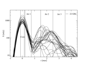
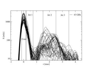
Figure 2: Intensity profiles of the VLBI images of BL Lac at 22 GHz (top) and 43 GHz (bottom), combining all epochs. The figure illustrates the flux density behaviour of the jet ridge-line at a resolution of 0.5 mas (22 GHz) and 0.3 mas (43 GHz) at P.A. $=195^{\circ}$. Each curve represents one epoch between 1997 and 2003. Vertical lines indicate the core and jet regions that were used to analyse the images.

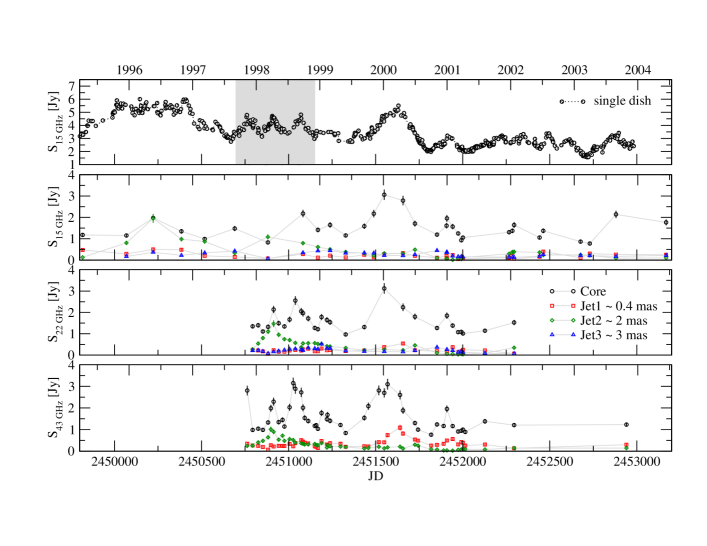
Figure 3: Flux density evolution of different portions of the VLBI core-jet structure of BL Lac at 15 GHz, 22 GHz, and 43 GHz compared with the 15 GHz single-dish light curve. Different symbols denote different separation from the core $r$ (see text for more details). The grey box highlights an example of a nice case study, where there are three equally bright flares, but the VLBI data reveals that contrary to the others the middle one was dominated by the jet and not by the core. Note that due to the rapid fading of the jet we do not show a Jet3 curve at 43 GHz.

We have tested several alternative positions with different sizes to check how the light curves change at different core distances. If we take measurements within a very small region, the integrated flux density goes down and the signal to noise ratio of the light curve decreases. On the other hand, if the region is too large, different jet components will overlap and smear out the variability. We find that the best choice is a small region close to the core, where flares from the core might be detectable with only a short time delay, as well as two slightly larger regions after the low emission gap to trace the flux density evolution farther downstream.

The core is represented by a circular region of 0.15 mas radius around the image centre, the first jet region corresponds to a core separation of $0.2\,{\rm mas}\leq r\leq 0.7$ mas, the second one to $1.5\,{\rm mas}\leq r\leq 2.5$ mas, and the third one to $2.5\,{\rm mas}\leq r\leq 3.5$ mas. We have tested several methods to obtain the corresponding light curves, including 1) the task IMSTAT in AIPS, which integrates the flux density of the image within a predefined rectangular region, 2) model fitting of Gaussian components in Difmap; and 3) integrating the flux density along the slices presented in Fig 2. Among the alternatives, we find that a quite accurate and flexible method is to extract the light curves by summing the delta-function components within the specified regions from the final CLEAN models produced with Difmap. Another advantage of this method is that one can easily change the limits of the regions and rerun the analysis. Since most of the data were reduced by various authors and the quality of the data is inhomogeneous, we estimate the flux density error to be 10%, which is typical for VLBI measurements. From our experience with the VLBA, 10% is a conservative assumption and the typical uncertainty at 15 GHz and 22 GHz might be as low as 5%. Our three VLBA+Effelsberg epochs (2002.03, 2002.51, and 2003.24) at 15 GHz have typical errors of 5% estimated from the gain corrections during the amplitude self-calibration.

Figure 3 shows the final VLBI light curves in comparison with the 15 GHz single-dish light curve from UMRAO. One can clearly see that the single-dish light curve is usually dominated by variability of the VLBI core, but occasionally parts of the jet reach or even overcome the core brightness. The latter is most evident at 15 GHz before mid 1998. Villata et al. (2004a) calculated the flux density ratio (a “hardness ratio,” which is comparable with the radio spectral index) between the 22 GHz and 5 GHz light curves and distinguished two different kind of flares. Flares that are more pronounced at higher frequencies are called hard flares (inverted or flat radio spectrum), while flares that are dominant at lower frequencies are called “soft flares” (steep radio spectrum).

From a comparison of Fig. 3 with Fig. 8 in Villata et al. (2004a), one can see that the hard flares are observed when the VLBI core is bright compared to the jet, while during soft phases the jet is relatively bright. For example, the second flare (1998.2) of the three equally bright flares in the single-dish light curve between 1997.7 and 1998.9 in Fig. 3 (grey box) is softer than the adjacent ones (cf. also Fig. 8 in Villata et al. 2004a). If we take a look at the VLBI light curves it becomes obvious that, although in the single-dish measurements the flares have a similar brightness, the 1998.2 flare has a large contribution from a brightening in the jet at about 2 mas core distance (jet2) and originates not only from the core. It seems therefore very important to know the jet contribution to the single-dish light curves if we intend to compare the radio variations with X-ray or optical light curves, since they are most likely dominated by the emission from the jet-base and not from the outer optically thin jet emission.

3.2 Radio spectral index

The single-dish radio spectral index $\alpha$ (defined as $S_{\nu}\propto\nu^{\alpha}$, where $S_{\nu}$ is the flux density at frequency $\nu$) was calculated for all adjacent frequency pairs between 5 GHz and 37 GHz with separation shorter than 3 days. This limit is usually fulfilled for data from the same observatory (5, 8, 15 GHz from UMRAO and 22 and 37 GHz from Metsähovi) and therefore reduces the sampling significantly only for the 15 GHz to 22 GHz spectral index. The mean time sampling for the radio light curves is typically of 10 days, but after 1990 the time sampling becomes much better ($\sim 5$ days). The spectral indices obtained for different pairs of frequencies (5/8, 8/15, 15/22, and 22/37 GHz) all follow the same behaviour in time. In Fig. 4 (top panel) we show the spectral-index curve between 8 GHz and 15 GHz ($\alpha_{8/15}$), which is the best sampled one. One can see that most of the flares are accompanied by a flattening of the spectrum. The flattening seems to peak shortly before the flare reaches its maximum. A comparison between the 43 GHz VLBI core flux density and $\alpha_{8/15}$ is shown in the bottom panels. The single-dish spectral index is able to trace the VLBI core variability in a very accurate way. We will test this using a discrete correlation function (DCF) in the next section.

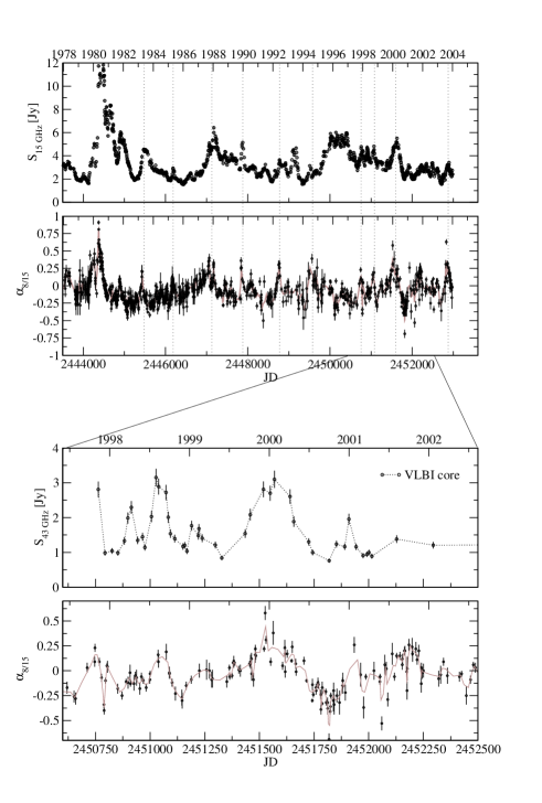
Figure 4: Top panels: Radio light curve at 15 GHz in comparison with the spectral-index curve between 8 GHz and 15 GHz. One can see that most of the flares are accompanied by a flattening of the spectrum. The vertical dotted lines mark some examples and help to guide the eye. Bottom panels: Zoom into the time range of the VLBI monitoring at 43 GHz. The grey line represents a three point average of the spectral-index curve. There is a close apparent correlation between the 43 GHz core flux density and $\alpha_{8/15}$ (see also Fig. 6).

The time evolution of the spectral index of the VLBI core and the inner 3 mas of the jet can be seen in Fig. 5. Shown are the ridge-line profiles of BL Lac across the spectral index VLBI maps between 22 GHz and 43 GHz along P.A. $195^{\circ}$. The spectral index maps were produced by aligning the two images on the brightest component. To reduce the effect of a potential core shift between the two frequencies, we convolved the images with a 0.7 mas circular beam. Since there are no strong spectral gradients visible in the core region that would indicate a core shift, we assume that the effect is negligible at the resolution of our images. The core spectrum in Fig. 5 is significantly flatter than the jet for most of the time especially when it is flaring (e.g., epoch 1998.61). It therefore seems reasonable that the variability of the single-dish radio spectral index is a good tracer for the variations in the VLBI core.

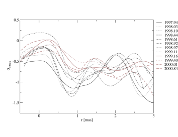
Figure 5: Ridge-line profiles of the spectral index maps between 22 GHz and 43 GHz showing the core and the inner 3 mas of the jet along P.A. $195^{\circ}$. The original images were tapered to the same resolution and convolved with a circular beam of 0.7 mas.

3.3 Cross-correlation

A cross-correlation of the single-dish light curves of BL Lac has already been performed by Villata et al. (2004a) using a DCF analysis (Edelson & Krolik 1988; Hufnagel & Bregman 1992). We will continue to use this method here. The authors found that the higher frequency radio variations lead those at lower frequencies by several days to a few months, depending on the frequency separation. In particular, the variations at the lowest frequency (5 GHz) lag the other frequencies by $\sim 40$ days (8 GHz), $\sim 59$ days (15 GHz), and $\sim 78$ days (22 GHz) with uncertainties of 5 to 10 days. These values were derived by calculating the centroid of the DCF near its peak. The corresponding uncertainties were estimated from variations of the time binning and the calculation of the centroid for cutoffs between 70% and 80% of the peak value. To complete the frequency coverage, we derive here also the DCF for the 5 GHz and 37 GHz frequency pair and find a time lag of $105\pm 15$ days. To be consistent with Villata et al. (2004a) all DCFs in this work are performed for the same time range, between JD=2446500 (March 1986) and JD=2453000 (December 2003), which excludes the highly pronounced radio flare in 1980. Such prominent events could lead to spurious peaks in the DCF analysis, since a peak would appear at every time lag at which it overlaps with a flare in the second light curve. We note that the time range that we use is shorter for the VLBI data, which are only available between 1995 and 2004. All DCF calculations were performed several times with different binning in time and over different time ranges. The plots shown here correspond to the versions that showed the most robust results. In most cases small changes did not affect the results significantly and, where larger changes were observed, these are discussed in the text.

Villata et al. (2004a) found a modest correlation between the optical light curve and the high-frequency radio ones with a radio time lag of about 100 days. Moreover they showed that a better correlation is found when comparing the optical variability with the spectral variations in the radio bands, which highlights radio flares that are more pronounced at higher frequencies. On the other hand, the radio spectral index and the VLBI core flux density (Fig. 4) also seem to agree very well. The corresponding DCF analysis supports the correlation (Fig. 6). There appears also a possible anti-correlation at about $-250$ days, but this is very likely due to the broad peak around 2000.0 overlapping with the dip at $sim2000.7$ (Fig. 4). Calculation of the centroid of the highest 3 points of the DCF gives a short time delay of about 4 days for the spectral index, but at a bin size of 60 days the uncertainties are too large to reliably measure such short delays. We thus performed cross-correlations between the optical $R$ band light curve and our VLBI core light curves. The results are shown in Fig. 7. The time sampling of the VLBI data is not as good as for the single-dish light curves. This might explain why the correlation is not so strong; however, all curves show a tentative correlation with a 50 to 100 day time lag. The strongest correlation is found with the 43 GHz core light curve, which is also the best sampled one.

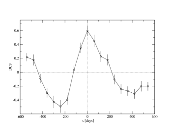
Figure 6: DCF of the 43 GHz VLBI core flux density (1997–2002) and the radio spectral index between 8 GHz and 15 GHz showing a good correlation with a possible short delay of the spectral index.

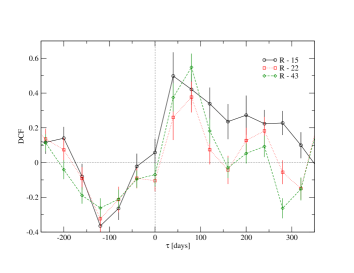
Figure 7: DCF of the optical $R$ band light curve with the VLBI core light curves at 15 GHz (1995–2003), 22 GHz and 43 GHz (1997–2002).

We obtain a better result from the cross-correlation of the optical data with the spectral indices. Figure 8 (top panel) shows the DCF for all four frequency pairs between 5 GHz and 37 GHz (1986–2003). Although the DCF peaks are below 0.6, the clear trend for shorter time delays at higher frequency pairs is consistent with the radio cross-correlations, which show that the higher frequencies lead the lower ones (Villata et al. 2004a). The secondary peaks with negative time delays most likely come from the regular pattern of optical flares after 1997, visible in Fig. 9, which appear at separations of a bit less than 1 year (6 flares in 5 years). Auto-correlations of both the optical light curve and the 22/37 GHz spectral index weakly show this periodicity if we analyse only the time-range after 1997, but the periodicity vanishes outside of this 5-year period. Therefore, we cannot rule out that the light curves of BL Lac sometimes show periodicities, but then it is only a short-term phenomenon. Periodicity analyses of BL Lac light curves performed by various authors have found periods between 2.5 yr and 4 yr, about 8 yr, and 15 yr to 20 yr for the radio (e.g., Kelly et al. 2003; Villata et al. 2004a), and about 1 yr, 5 yr, 7  to 8 yr, 10 yr, and 15 yr in the optical (e.g., Hagen-Thorn et al. 1997; Villata et al. 2004a), at different significance levels. It is evident that further investigations are needed before we can draw any conclusions regarding the presence of true, persistent periodicities.

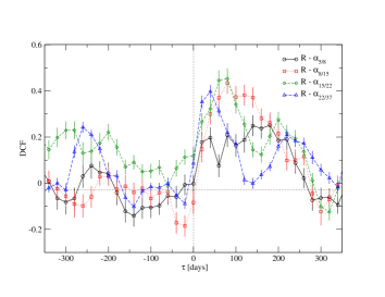
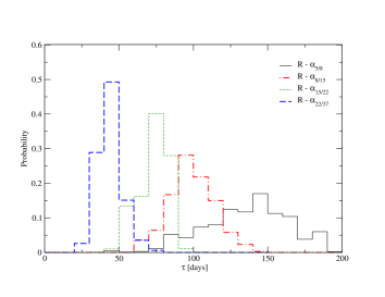
Figure 8: Top panel: DCF of the optical $R$ band light curve with all spectral index pairs between 5 GHz and 37 GHz (1986–2003). Although the correlations reach a maximum peak value of only about 0.5, there is a clear trend to shorter time delays for higher frequencies. Bottom panel: Probability plot for the DCF peaks resulting from the correlation between optical data and radio spectral indices derived from 1000 Monte Carlo simulations.

The formal statistical significance of the found time lags using the DCF analysis in this work is not easy to asses. In general the statistical significance of a correlation depends on the number of points that contribute to the calculation of the time lag (e.g, Peterson 2001). Since the number of points that contribute to the peak value of the DCF in our analysis always exceeds 100, all peaks higher than 0.25 have to be considered as being significant at a confidence level of about 98%. Therefore we carefully checked by eye how many flares with which amplitude in the light curves contribute to the correlation and if there are any dominant flares which could strongly affect the DCF (see also Fig. 9). Hence we might call the $R-\alpha_{22/37}$ DCF with a peak value of 0.4 better than the correlation between $\alpha_{8/15}$ and the 43 GHz VLBI core light curve with a peak value 0.6, because the larger time interval and better sampling of $R-\alpha_{22/37}$ correlation makes it more reliable. A summary of the used parameters for all DCFs is given in Table 2.

Another method to test the robustness of the DCF peaks is to perform Monte Carlo simulations in which the curves are randomly modified within the measured uncertainties and only subsets of the data are correlated – a technique known as “flux redistribution/random subset selection” (FR/RSS; Peterson et al. 1998; see also Raiteri et al. 2003). We used this method to test the peaks of the $R--\alpha$ cross-correlation (Fig. 8 (top)) through 1000 Monte Carlo simulations. In Fig. 8 (bottom) the fraction of occurrence of the 75% centroid values of all Monte Carlo realizations for the four DCFs are given. The histogram shows that the time delay and the uncertainty of the DCF between the $R$ band and the radio spectral index decreases towards higher radio frequencies.

Table 2: Summary of cross-correlation parameters. Columns contain the frequency pairs (numbers denote radio frequencies in GHz and a “V” marks data obtained from VLBI images), time interval of correlation (MJD=JD-2400000), binning interval, DCF peak value, time-lag of the peak, time lag of the 75% centroid, and a reference to the corresponding figure.

type	time int.	bin	DCF	$\tau_{\rm peak}$	$\tau_{\rm cent.}$	Fig.
	[MJD]	[days]		[days]	[days]
$\alpha_{8/15}$–43V	50760–52950	60	0.60	0	0	6
$R$–15V	49800–53100	40	0.50	40	58	7
$R$–22V	50760–51080	40	0.38	80	64	7
$R$–43V	50760–52600	40	0.55	80	61	7
$R$–$\alpha_{5/8}$	46500–52600	20	0.26	180	148	8
$R$–$\alpha_{8/15}$	46500–52600	20	0.41	80	93	8
$R$–$\alpha_{15/22}$	46500–52600	20	0.45	80	71	8
$R$–$\alpha_{22/37}$	46500–52600	20	0.39	40	39	8

To summarize: a fair correlation was found between $S_{\rm core}$ and the radio spectral index with no measurable time delay, which suggests that the radio spectral index is a good indicator for the VLBI core variability. A tentative direct correlation is seen between $S_{\rm core}$ and the optical light curve with radio time lags of less than 100 days. This, together with the correlation between the optical flux and the radio spectral index, provides evidence that the optical variability is indeed correlated with the radio emission of the VLBI core.

In Table 3 we summarize the estimated time delays for the five radio frequencies during the time range of 1986 and 2003. Since the flattening of the spectrum appears when the higher frequency light curve rises earlier and/or faster than the lower frequency one, the variability of the spectral index should represent the core variability at the higher frequency. Therefore, we attribute the time lag between the optical emission and the spectral index to the highest radio frequency. The delay of the 5 GHz variations, the lowest frequency light curve in the analysis, is derived by adding the time lag between the 5 GHz and 8 GHz radio light curves to the $R$–8 GHz time lag. This procedure might lead to small shifts of the derived time lags, since the shape and peak of the spectral index variations are a combination of both frequencies, but tests with different frequency pairs that are more widely separated (e.g., 15/37 GHz or 8/37 GHz) support this approach and yield shifts of less than 5 days. This is well within the 1 $\sigma$ errors derived from the Monte Carlo realizations.

Table 3: Time lags, $\tau$, measured between the optical and the radio variations. The values are derived from the correlation of the optical emission with the radio spectral indices (see text for details).

opt – $\nu$ [GHz]	$\tau$ [days]
$R$ – 5	$175\pm 30$
$R$ – 8	$136\pm 28$
$R$ – 15	$99\pm 15$
$R$ – 22	$71\pm 10$
$R$ – 37	$44\pm 10$

Figure 9 illustrates the good agreement between the optical light curve and the radio spectral index ($\alpha_{8/15}$). In this figure the spectral index is shifted by –99 days according to the $R$–15 delay (Table 3). Moreover, to make the comparison easier, we plot the spectral index by $(\alpha_{8/15}+0.8)^{3}$ (top) and $(\alpha_{8/15}+0.8)^{4}$ (bottom), so that all values are positive and the peaks are enhanced. One can see that the curves agree fairly well during the last $\sim 10$ years (bottom panel).

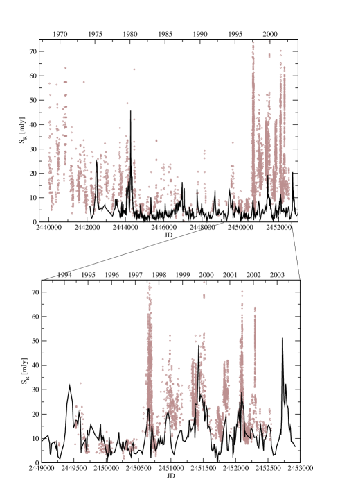
Figure 9: Optical light curve vs. radio spectral index ($\alpha_{8/15}$). The spectral index is shifted by –99 days. To make the comparison easier we represent the spectral index by $(\alpha_{8/15}+0.8)^{3}$ (top) and $(\alpha_{8/15}+0.8)^{4}$ (bottom), so that all values are positive and the peaks are enhanced. The curve is smoothed with a three point average to reduce the noise. Top: All data. Bottom: Only the last 10 years with the best sampled data.

4 Discussion

4.1 Optical-radio time delays

The long observational history of BL Lac led to several attempts to search for radio-optical correlations. Some of these found correlations with radio time delays of several hundred days (Pomphrey et al. 1976; Hufnagel & Bregman 1992; Tornikoski et al. 1994b; Clements et al. 1995; Hanski et al. 2002). Sometimes simultaneous events were reported (Balonek 1982; Tornikoski et al. 1994a). A common result is that there are periods where radio and optical variations correlate better and others where the correlation seems to disappear. The correlations found here (Sect. 3.3) are calculated for data from 1986 to 2003, thus excluding the large outburst in 1980. Although the sampling is not homogeneous, it seems that the optical emission underwent a period of suppressed activity from 1981 to early 1997 (Fig. 9), during which flares were less frequent and not so pronounced. Such a period is visible neither in the radio light curves nor in the radio spectral index (Fig. 4).

By constraining the DCF analysis on smaller time ranges we test how the time delays change with time. This was done exemplarily for the cross-correlation of the R band fluxes with $\alpha_{8/15}$. The data between 1986 and 1989 are not so well sampled, but although the DCF results become less significant, they confirm the previous findings. During the period before 1986 a broad peak at about 300 days is found, which is in good agreement with the results from the studies of data up to 1992 (Pomphrey et al. 1976; Hufnagel & Bregman 1992; Tornikoski et al. 1994b; Clements et al. 1995; Hanski et al. 2002). During the period of weak optical variability (from 1986 to early 1997) a small peak around zero time delay indicates some simultaneous events (Balonek 1982; Tornikoski et al. 1994a), but in general the DCF during this time shows no peak above 0.25. Finally the most recent data (1997 to 2003), characterized by the high optical activity, are dominated by a peak at around 100 days. The fact that both Villata et al. (2004a) and our new analysis detected this 100-day time delay for data obtained from 1986 until now, demonstrates that the most recent correlation seems to dominate over that found in the previous period of weak variability. However, the time range used here is not dominated by a major outburst, but rather consists of several flares in the optical (6–7 major events after 1997 and about the same number of minor flares before 1997), and the variability of the spectral index displays nearly the same amplitude throughout the whole period. Therefore, the optical-radio delays found in Sect. 3.3 seem to represent the result of a true correlation in the variability behaviour of BL Lac over at least the last 10 years of our dataset.

4.2 Frequency dependence of the delay

Frequency dependent time delays in radio flares are commonly related to a combination of optical depth and travel time along the jet. Evolving flares first appear in the inner jet region at the highest frequencies and, as the perturbations (VLBI components) travel down the jet, the flares become visible at successively lower frequencies where the optical depth of synchrotron self-absorption decreases to $\tau_{\rm s}\sim 1$ at that frequency. For a given magnetic field strength ($B(r)$) and electron energy distribution scale factor ($N(r)$), the corresponding $\tau_{\rm s}$ is (e.g., Lobanov 1998):

$$\tau_{\rm s}=C_{2}(\alpha)N_{1}\left(\frac{eB_{1}}{2\pi m_{\rm e}}\right)^{\epsilon}\frac{\delta^{\epsilon}\phi_{0}}{r^{(em+n-1)}\nu^{\epsilon+1}}$$ (1)

Here $m_{\rm e}$ is the electron mass, $e$ is the electron charge, $\epsilon=3/2-\alpha$, $\alpha$ is the optically thin synchrotron spectral index, and $m$ and $n$ are the power-law exponents of the radial distance dependence of the magnetic field and $N(r)$, respectively (e.g., Lobanov 1998). The observed jet opening angle is $\phi_{0}=\phi\csc\theta$. The factor $C_{2}(\alpha)$ is described in Blumenthal & Gould (1970), and $C_{2}(-0.5)=8.4\cdot 10^{10}$ in cgs units. Setting $\tau_{\rm s}$ to unity gives us an estimate of the distance from the convergence point of the jet to the core as observed at frequency $\nu$.

Hence, we should be able to measure a frequency-dependent core position in VLBI images: for a conical jet geometry the shift is given by $r\propto\nu^{-1/k_{\rm r}}$, where $k_{\rm r}=[(3-2\alpha)m+2n-2]/(5-2\alpha)$ (e.g., Lobanov 1998). For the case of equipartition between the magnetic field and electron energy densities, the simplest choice of $m=1$ and $n=2$ (Königl 1981) leads to $k_{\rm r}=1$ independent of the spectral index (Lobanov 1998). Larger values are reached in regions with steeper pressure gradients than if, e.g., the electrons suffer adiabatic energy losses without reacceleration (Marscher 1980). Thus, taking measurements of the core shift between several frequencies allows to estimate $k_{\rm r}$ along the jet (e.g., Lobanov 1998; Kadler et al. 2004).

If the radio time lags are also due to opacity effects and the flare travels at a constant speed, then they should also be proportional to $\nu^{-1/k_{\rm r}}$. Recent kinematic studies on high frequency VLBA data of BL Lac have consistently derived jet speeds with a bulk Lorentz factor of about 7 and an angle to the line of sight of $\sim 12^{\circ}$, with only minor deviations (Denn et al. 2000; Reynolds et al. 2003; Stirling et al. 2003; Kellermann et al. 2004; Jorstad et al. 2005). We therefore assume that the Lorentz factor and angle to the line of sight are more or less constant, and that the time delays are proportional to the distance between the two emitting regions. E.g., a time delay, $t^{\prime}$, of 10 days would then correspond to a distance, $r$, of about 0.06 pc ($r=t\,\beta\,c$, with $\beta=\sqrt{1-\frac{1}{\gamma^{2}}}$ and $t=\gamma\,t^{\prime}$).

In Fig. 10 we plot the measured radio lags with respect to both the 37 GHz data and to the optical data vs. frequency. A power-law fit represents the data reasonably well in both cases (reduced $\chi^{2}<1$) and there it seems that the assumption of a constant jet speed holds at least in the radio regime. It is important to note that the value of $k_{\rm r}$ strongly depends on the absolute time lag, i.e. on the distance to the base of the jet, which might be not far from the central engine. Although the optical emission could be emitted close to the foot point of the jet, we should consider that this region is still at some considerable distance from the central engine. In this case $k_{\rm r}$ would be larger. If, on the other hand, the jet speed between the radio and the optical emitting regions is not constant, the simple assumption of $\tau\propto\nu^{-1/k_{\rm r}}$ is invalid. However, it seems that at least in the radio regime the speed is constant and we can infer that $k_{\rm r}$ is likely larger than 1.1. This implies that the gradients in jet parameters are steeper than in the case of equipartition with $m=1$. Our result is, on the other hand, consistent with a freely expanding jet with adiabatic energy losses, in which case $n=(2/3)(3-2\alpha)$ (Marscher 1980) and $k_{\rm r}=(15-14\alpha)/[3(5-2\alpha)]$ for $m=1$, or $k_{\rm r}\approx 1.2$ for $\alpha\approx-0.5$.

Figure 10: Measured time lags vs. frequency. The circles and dashed line represent the measured time lags and the corresponding fit with respect to the optical emission, while the squares and dotted line denote time lags and fit with respect to the 37 GHz light curve.

4.3 Connection with jet components

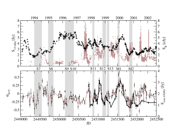
Figure 11: Top: Optical (grey squares) and radio (black circles) light curves in comparison with the ejection dates of new superluminal jet components, which are highlighted as grey vertical bars. The width of each bar corresponds to the uncertainty of the ejection date. Bottom: Ejection dates vs. radio spectral index (black circles and grey trend-line) and the 43 GHz core flux density (black squares and line). The ejection dates are taken from Denn et al. (2000), Stirling et al. (2003) (S7 to S13), and Marscher et al. (2004) (M1 and M2). Only some of the new components seem to be connected with events in the light curves.

Since outbursts (especially at mm wavelengths) are often related to the ejection of superluminal jet components (e.g, Otterbein et al. 1998; Savolainen et al. 2002), we have compared our radio and optical light curves and the spectral index, $\alpha_{8/15}$, with the ejection dates of jet components reported in the literature. Figure 11 illustrates this comparison. There is no obvious connection among the events, but some new components are led by an optical flare or followed by an increase in the radio. We also tested whether we could find any evidence for a connection between the ejections and flares by calculating the variations in the flux density at different frequencies and the spectral indices for times shortly before and after the ejection, but no clear trend could be found. There is always a significant fraction of the components that does not show the expected behaviour. However, this kind of analysis might be affected by the relatively large errors in the dates of the earlier ejections (S7 to S10) and the fact that some components appear very close together (S9/S10 and S12/S13). Furthermore, the light curves are generally composites of multiple events, some of which are declining in flux while others are rising. This can render individual flares unnoticed in the total-flux light curves.

The best agreement can be seen for the two newest components M1 and M2. They appear accompanied by an optical flare and are followed by a flare and flattening of the spectrum at radio frequencies. Since previous works have also reported a good agreement between the appearance of flares and the ejection of components from S1 up to S7 (e.g., Mutel et al. 1990; Aller 1999), it might be that the dates of S8 to S13 are not so well determined. Although S7, S11, and S12 can be identified with minor radio flares and a flattening of the spectrum, there are several large flares in the optical and radio light curves at 1997.6, 1998.4 and 1999.5 that seem to be unrelated to any new component. It will be interesting to see if the ongoing densely sampled VLBI monitoring will find corresponding components to the pronounced optical flares around 2001.5 and 2002.1.

As mentioned earlier, one should also expect to see a sign of the travelling jet components in the different parts of the VLBI light curves. After a flare in the VLBI core, a new component should brighten the jet after some time at every measured distance while it passes by. Unfortunately, the jet flux density is either too low or the time sampling is insufficient to reliably detect such events. In addition, the ejection of several components or the appearance of many flares in a short time can confuse the picture. A good example of the evolution of a new jet component is M1 (Fig. 11) ejected in 1999.95 (JD=2451527). The corresponding flare is a nicely separated event and from Fig. 3 one can see that, some time after the peak in the core, the inner jet ($r\approx 0.4$ mas) brightens at 43 GHz and 22 GHz, while later it appears at 2 mas and finally at 3 mas separation from the core. Since not all frequencies were observed simultaneously and in order to see better the evolution, we have converted the flux densities at 15 GHz and 43 GHz of the core and jet to 22 GHz according to their measured spectral index and show these together in Fig. 12. The plotted data points are three-point averages to smooth the residual differences, and the error bars correspond to their standard deviations. Parabolic fits to the data illustrate the appearance of the component at the different jet positions. The calculated speed of the component from the peaks in the light curves is about (2–4) mas/yr or $\beta_{\rm app}\approx$ (12–19) $c$. This is somewhat higher than the speeds of 5 $c$ to $9\,c$ from kinematic studies reported thus far (Denn et al. 2000; Stirling et al. 2003; Kellermann et al. 2004; Jorstad et al. 2005), but since we have combined all frequencies in order to be able to fit the peak, our values might be more uncertain.

Figure 12: VLBI light curves of the radio flare in early 2000. To better follow the flare evolution in both time and space, all fluxes are converted to 22 GHz according to their spectral index and combined in a three point average. One can follow the propagation of the core outburst along the jet. The ejection dates of new VLBI components are marked by arrows and correspond to M1 in 1999.95 and M2 in 2000.81 reported by Marscher et al. (2003).

Another jet component ejection (M2) is reported for 2000.81 (JD=2451841; Marscher et al. 2003) and the related radio flare is also visible in Fig. 12. There is a sharp core peak at JD=2451920 and some time later a peak in the $r\approx 0.4$ mas light curve. Unfortunately, the dense VLBI monitoring ends in early 2001 and one cannot follow the flare further. However, both ejections are accompanied or led by a bright optical state, which suggests that the correlated optical-radio variability observed here is also related to the ejection of jet components.

During 1999 and 2000 BL Lac was the target of several RXTE (Marscher et al. 2004) and BeppoSAX (Ravasio et al. 2002, 2003; Böttcher et al. 2003) observations. Interestingly, the source was caught in very different states. The RXTE light curve covers nearly the whole period of 1999 to 2001 with dense sampling. In particular, during the ejection in 2000.81 strong variability is observed together with a softening of the X-ray spectrum (Marscher et al. 2004). This is also confirmed by the BeppoSAX observations from October 31 to November 2, 2000 (JD$\sim$2451850; Ravasio et al. 2003; Böttcher et al. 2003), which show an unusually strong soft spectral component between 0.2 keV and about 10 keV. Unfortunately, the flare/ejection in 1999.95 was not covered by RXTE, while the BeppoSAX observations of December 5–6 (JD$\sim$2451518) obtained several days before the extrapolated ejection date showed no sign of a soft component, but a hard spectrum similar to that observed in July 2000. Another BeppoSAX observation on June 5–7, 1999 (JD$\sim$2451336) shows again a small soft component between 0.2 keV and about 3 keV (Ravasio et al. 2002), which seems also visible as a small enhancement in the RXTE light curve and spectrum (Marscher et al. 2004). This small X-ray flare is also followed by optical and radio flares, but no new jet component has been reported. However, this might be due to confusion with the two earlier ejections of components S12 and S13, which were separated by only 0.3 yr.

Although further coordinated observations are needed to complete the picture, the very well sampled period from 1999 to 2001 already reveals some very interesting similarities in the variability behaviour from X-ray to radio wavelengths, which are also visible as changes in the source VLBI structure. The missing soft-spectrum component in the BeppoSAX observations of 1999.92 might blear the claim of a correlation, but given that the typical uncertainty in the ejection dates is about 0.2 yr and the soft X-ray tail is potentially a short-lived phenomenon, more observations yielding better statistics are necessary.

4.4 A possible jet scenario

Due to the combination of the structural analysis using VLBI light curves and the single-dish observations, we are confident that the emission from the VLBI core, presumably close to the base of the jet, is responsible for the correlated variability observed at optical and radio wavelengths, and possibly also up to X-ray frequencies (Marscher et al. 2004). The mechanisms that can explain blazar variability are still the subject of discussion. Possibilities suggested in the literature include shocks in jets (Marscher & Gear 1985; Aller et al. 1985; Marscher 1996), and flares introduced by the lighthouse effect from changes in the direction of forward beaming caused, e.g., by helical trajectories of plasma elements (Camenzind & Krockenberger 1992), by a precessing binary black-hole system (Begelman et al. 1980; Sillanpaa et al. 1988), or by the rotation of a helical jet (Villata et al. 1998; Villata & Raiteri 1999; Ostorero et al. 2004). Furthermore, variability caused by colliding relativistic plasma shells has been considered (Spada et al. 2001; Guetta et al. 2004).

Regardless of the variability origin, the VLBI observations of BL Lac indicate a bent path of the jet. The trajectories of several jet components have been well modelled and predicted by helical jet models (Denn et al. 2000; Stirling et al. 2003). A bent jet path could also explain the region of low emission around 1 mas from the core noticed in Sect. 2.2 (Fig. 2). One can see strong variability in both the core and the jet at core separations larger than 1 mas, but never between 0.7 mas and 1 mas. Since the spectral index does not show any evidence for absorption, a natural explanation would be reduced Doppler boosting either from a misalignment between the jet direction and our line of sight or from a change in the jet speed.

A possible scenario that could account for the observed variability behaviour, especially the changing variability pattern between optical and radio emission on timescales of several years, would be a helical jet structure that is precessing or rotating. Since the optical emission is most likely produced on small scales, a small misalignment could beam the emission less favourably, which could explain the low optical state with suppressed variability from 1981 to early 1997 (see Sect. 4.1). On the contrary, the radio emission, coming from all along the jet, would be always strongly beamed in some part of the helical path and therefore would not suffer the less intense beaming of the optical component (e.g., Rieger 2004, 2005 and references therein). The only beaming-suppressed region at radio frequencies would be the emission gap in the inner jet. In this case the gap might move or disappear with time and could be used by future VLBI studies to prove or disprove the rotating jet scenario.

5 Summary

We have presented an analysis of a VLBI data set that includes 108 images at 15 GHz, 22 GHz, and 43 GHz obtained between 1995 and 2003. The aim has been to disentangle the different components contributing to the single-dish radio light curves. Inspection of the VLBI light curves corresponding to different regions of the jet reveals that the radio single-dish light curves indeed display the sum of the emission from the core and from some prominent jet features. In some cases these jet features become as bright as, or even brighter than, the core itself. This leads to a complication of the cross-correlation between the radio light curves and other wavebands where the emission might come from the core region alone.

We find that the spectral variability that is present in the single-dish light curves can trace the variability of the VLBI core, and therefore enables a study of the long-term variability of the radio core even when VLBI data are not available. Using this result, we find a fair correlation between the variations of the radio spectral index and the $R$-band optical light curve with radio delays of about 50 to 180 days depending on the frequency separation. (Here we attribute the delay measured from the spectral index between two frequencies to the higher frequency. This seems justified as the flattening and also the peak of the spectral index curve is mainly due to the earlier and faster rise of the flare at the higher frequency.) Owing to the shorter time range and the sparser sampling, the radio-optical correlation is weaker when considering the VLBI core light curves at 22 GHz and 43 GHz directly, but the delays found are comparable to those of the spectral indices. The resulting time lags are also consistent with those from the cross-correlations performed by Villata et al. (2004a).

Assuming that the radio time lags are due to an optical depth effect of synchrotron self-absorption and that flares propagate along the jet at a constant speed, we obtain a power-law dependence of the time lag on frequency that suggests that the jet does not maintain equipartition of magnetic and particle energy densities as it expands. The radio-optical correlation is most prominent before 1981 and after 1997. During the 16 years in between, we observe only moderate variability in the optical and the correlation with the radio almost disappears. Stirling et al. (2001) have suggested a precessing jet nozzle for BL Lac to explain their observations, which may imply that the optical variability is also orientation dependent. This in turn, depending on the geometry, could also affect the correlation with the radio regime. This would lead to a natural explanation of the changing appearance of correlated variability: since the optical emission likely originates on small scales, a minor misalignment could beam the emission less favourable. On the other hand, the beamed radio emission could still repeatedly approach our line of sight along its helical path farther down the jet, so the precession or rotation might modify the amplitude of the variability pattern without leading to a vanishing flux as in the optical bands (e.g., Rieger 2004, 2005). A bent jet path could also explain the low emission region in the jet around 1 mas from the core. A movement or the disappearance of the gap in future VLBI studies, could therewith be used to prove or disprove a rotation of the bent jet path.

[x]lcrrcccc Observing log. Given are the observing epoch, frequency, beam size and orientation, total flux in the image (S_tot), peak flux density (S_max), rms noise level (S_rms), and the references where the data was first published.

Epoch $\nu$ Beam S_tot S_max S_rms Ref.
[GHz] [mas x mas] [^∘] [Jy] [Jy] [mJy]

Table 0 – continued from previous column
Epoch $\nu$ Beam S_tot S_max S_rms Ref.
[GHz] [mas x mas] [^∘] [Jy] [Jy] [mJy]

Continued on next page

1995.27 15 $0.50\times 0.88$ $2.9$ 3.30 1.79 2.4 (1)
1995.96 15 $0.53\times 0.97$ $0.9$ 5.01 2.04 2.5 (1)
1996.38 15 $0.51\times 0.90$ $-4.1$ 5.67 2.68 2.4 (1)
1996.82 15 $0.46\times 0.86$ $-2.6$ 3.84 1.77 3.2 (1)
1997.19 15 $0.58\times 1.00$ $7.1$ 3.21 1.49 1.5 (1)
1997.66 15 $0.56\times 0.91$ $12.4$ 2.97 1.70 1.5 (1)
1998.18 15 $0.50\times 1.00$ $8.2$ 2.68 1.06 3.8 (1)
1998.73 15 $0.57\times 0.87$ $-16.0$ 4.07 2.48 0.7 (5)
1998.97 15 $0.59\times 0.71$ $-3.0$ 2.98 1.54 0.7 (5)
1999.16 15 $0.63\times 0.78$ $6.5$ 3.26 1.88 0.6 (5)
1999.40 15 $0.60\times 0.81$ $6.2$ 2.38 1.30 0.7 (5)
1999.70 15 $0.55\times 0.77$ $-14.1$ 2.75 1.71 0.6 (5)
1999.85 15 $0.59\times 1.08$ $-3.3$ 3.31 2.34 1.3 (1)
2000.01 15 $0.56\times 0.79$ $-16.1$ 4.23 3.32 0.7 (5)
2000.31 15 $0.55\times 0.74$ $-4.7$ 4.18 3.16 0.6 (5)
2000.49 15 $0.56\times 1.00$ $16.7$ 3.23 1.96 0.5 (4)
2000.84 15 $0.57\times 0.97$ $27.1$ 2.14 1.32 0.4 (4)
2000.99 15 $0.54\times 0.94$ $-16.3$ 2.59 1.82 1.1 (1)
2001.00 15 $0.47\times 1.46$ $-6.0$ 2.83 2.08 0.8 (4)
2001.09 15 $0.49\times 1.27$ $-10.9$ 2.46 1.79 1.1 (4)
2001.17 15 $0.52\times 1.37$ $-1.8$ 1.92 1.35 0.9 (4)
2001.22 15 $0.57\times 1.02$ $33.8$ 1.78 1.14 0.3 (4)
2001.25 15 $0.54\times 1.44$ $-1.1$ 1.96 1.26 0.6 (4)
2001.97 15 $0.48\times 0.92$ $1.6$ 2.34 1.44 0.7 (1)
2002.03 15 $0.32\times 0.64$ $-33.2$ 2.62 1.40 0.4 (6)
2002.05 15 $0.85\times 1.15$ $29.3$ 2.75 1.79 0.6 (5)
2002.45 15 $0.52\times 0.79$ $-18.1$ 2.18 1.24 0.7 (2)
2002.51 15 $0.24\times 0.55$ $-20.4$ 2.52 1.38 0.5 (6)
2003.10 15 $0.51\times 0.76$ $-0.1$ 1.75 0.98 0.5 (2)
2003.24 15 $0.29\times 0.46$ $-35.8$ 1.73 0.80 0.3 (6)
2003.65 15 $0.48\times 0.71$ $0.8$ 3.11 2.40 0.7 (2)
2004.44 15 $0.53\times 0.73$ $-9.3$ 2.73 2.01 0.7 (2)
1997.94 22 $0.39\times 0.84$ $-14.1$ 2.79 1.54 1.2 (4)
1998.03 22 $0.45\times 0.87$ $-8.0$ 3.06 1.51 1.1 (4)
1998.10 22 $0.34\times 0.85$ $-11.3$ 2.81 1.21 1.3 (4)
1998.18 22 $0.36\times 1.00$ $1.9$ 2.90 1.42 1.6 (4)
1998.27 22 $0.35\times 0.85$ $-8.2$ 6.60 3.36 2.2 (4)
1998.35 22 $0.36\times 0.83$ $-7.4$ 3.17 1.58 1.5 (4)
1998.44 22 $0.35\times 0.87$ $-8.6$ 2.79 1.48 1.4 (4)
1998.52 22 $0.33\times 0.97$ $-13.6$ 3.22 1.82 1.5 (4)
1998.61 22 $0.36\times 0.87$ $-10.4$ 3.97 2.71 2.1 (4)
1998.73 22 $0.42\times 0.64$ $-17.8$ 3.25 2.13 1.0 (5)
1998.82 22 $0.35\times 0.93$ $-21.4$ 3.30 1.88 1.4 (4)
1998.92 22 $0.36\times 0.88$ $-14.8$ 2.72 1.44 1.5 (4)
1998.97 22 $0.48\times 0.57$ $-5.9$ 2.52 1.38 0.6 (5)
1999.03 22 $0.38\times 1.02$ $-13.2$ 3.72 2.07 1.1 (4)
1999.11 22 $0.36\times 0.82$ $-8.3$ 2.82 1.79 1.6 (4)
1999.16 22 $0.44\times 0.56$ $1.6$ 2.83 1.72 0.5 (5)
1999.41 22 $0.41\times 0.58$ $-5.5$ 1.93 1.06 0.6 (5)
1999.70 22 $0.39\times 0.64$ $-26.4$ 2.07 1.37 0.7 (5)
2000.01 22 $0.43\times 0.59$ $-15.7$ 4.32 3.43 0.5 (5)
2000.31 22 $0.43\times 0.56$ $-8.1$ 3.76 2.76 0.5 (5)
2000.49 22 $0.40\times 0.74$ $12.8$ 3.20 2.02 1.3 (4)
2000.84 22 $0.45\times 0.69$ $31.4$ 2.20 1.43 0.8 (4)
2001.00 22 $0.37\times 0.96$ $-4.0$ 2.65 2.07 1.3 (4)
2001.09 22 $0.38\times 0.84$ $-13.3$ 2.38 1.65 1.5 (4)
2001.17 22 $0.40\times 0.94$ $-1.9$ 1.69 1.20 1.1 (4)
2001.22 22 $0.46\times 0.78$ $33.7$ 1.98 1.34 0.7 (4)
2001.25 22 $0.39\times 0.98$ $-4.8$ 1.86 1.21 0.8 (4)
2001.59 22 $0.37\times 0.63$ $-11.3$ 1.88 1.34 0.7 (5)
2002.05 22 $0.65\times 0.92$ $24.0$ 2.28 1.61 0.9 (5)
1997.86 43 $0.17\times 0.43$ $-10.5$ 3.67 2.74 2.1 (4)
1997.94 43 $0.18\times 0.44$ $-10.2$ 1.75 0.98 1.8 (4)
1998.03 43 $0.23\times 0.46$ $-9.1$ 2.02 1.04 1.1 (4)
1998.10 43 $0.17\times 0.43$ $-12.2$ 1.93 0.97 1.6 (4)
1998.18 43 $0.17\times 0.53$ $-2.7$ 2.30 1.33 1.8 (4)
1998.23 43 $0.17\times 0.33$ $9.9$ 3.49 1.96 1.0 (3)
1998.27 43 $0.18\times 0.44$ $-10.2$ 3.56 2.17 1.9 (4)
1998.35 43 $0.16\times 0.44$ $-10.5$ 2.35 1.30 2.4 (4)
1998.41 43 $0.16\times 0.32$ $-14.6$ 2.70 1.35 0.6 (3)
1998.44 43 $0.18\times 0.44$ $-9.4$ 2.01 1.13 2.1 (4)
1998.52 43 $0.17\times 0.57$ $-15.6$ 3.21 1.96 1.8 (4)
1998.58 43 $0.16\times 0.28$ $1.1$ 4.28 2.98 0.8 (3)
1998.61 43 $0.19\times 0.43$ $-10.6$ 3.85 2.80 1.8 (4)
1998.70 43 $0.17\times 0.56$ $-17.3$ 3.88 2.65 1.4 (4)
1998.73 43 $0.20\times 0.32$ $-25.9$ 3.07 1.90 0.9 (5)
1998.76 43 $0.19\times 0.30$ $-11.5$ 2.50 1.44 0.7 (3)
1998.82 43 $0.17\times 0.47$ $-19.3$ 2.33 1.34 1.7 (4)
1998.92 43 $0.21\times 0.49$ $-23.6$ 1.99 1.18 1.4 (4)
1998.94 43 $0.19\times 0.30$ $-13.4$ 2.00 1.14 0.7 (3)
1998.97 43 $0.21\times 0.26$ $-11.3$ 1.86 0.99 0.7 (5)
1999.03 43 $0.17\times 0.60$ $-11.8$ 2.96 1.71 1.6 (4)
1999.11 43 $0.17\times 0.42$ $-9.7$ 2.05 1.47 1.7 (4)
1999.12 43 $0.19\times 0.32$ $-13.9$ 2.71 1.64 0.6 (3)
1999.16 43 $0.21\times 0.27$ $-1.1$ 2.31 1.38 0.6 (5)
1999.32 43 $0.18\times 0.26$ $7.8$ 2.10 1.19 1.2 (3)
1999.41 43 $0.23\times 0.39$ $-18.7$ 1.50 0.84 0.7 (5)
1999.70 43 $0.19\times 0.35$ $-30.0$ 2.12 1.50 0.7 (5)
1999.76 43 $0.20\times 0.38$ $-16.8$ 2.73 2.00 1.2 (3)
1999.93 43 $0.20\times 0.38$ $-15.9$ 3.68 2.76 1.0 (3)
2000.01 43 $0.23\times 0.31$ $-9.7$ 3.34 2.58 0.9 (5)
2000.06 43 $0.19\times 0.26$ $7.2$ 4.21 3.00 1.7 (3)
2000.26 43 $0.18\times 0.28$ $1.5$ 4.17 2.45 1.0 (3)
2000.31 43 $0.19\times 0.26$ $2.0$ 2.95 1.80 0.9 (5)
2000.49 43 $0.21\times 0.37$ $20.7$ 2.39 1.37 1.6 (4)
2000.54 43 $0.18\times 0.30$ $-6.3$ 2.03 0.97 0.8 (3)
2000.75 43 $0.19\times 0.32$ $-8.8$ 1.47 0.74 0.8 (3)
2000.84 43 $0.23\times 0.35$ $32.5$ 1.88 1.23 1.7 (4)
2000.94 43 $0.23\times 0.33$ $28.3$ 1.73 1.19 1.1 (3)
2001.00 43 $0.18\times 0.49$ $-4.6$ 2.83 1.98 1.2 (4)
2001.09 43 $0.18\times 0.44$ $-12.6$ 1.94 1.18 1.7 (4)
2001.17 43 $0.17\times 0.49$ $-4.4$ 1.46 0.92 1.5 (4)
2001.22 43 $0.21\times 0.36$ $33.4$ 1.61 0.99 1.2 (4)
2001.25 43 $0.19\times 0.48$ $-3.7$ 1.63 1.02 1.5 (4)
2001.28 43 $0.17\times 0.29$ $-2.6$ 1.44 0.83 0.6 (3)
2001.59 43 $0.26\times 0.46$ $13.1$ 1.99 1.48 1.0 (5)
2002.05 43 $0.33\times 0.57$ $33.3$ 1.73 1.27 1.4 (5)
2003.82 43 $0.20\times 0.38$ $-22.1$ 1.88 1.27 0.7 (5)
Note: (1) VLBA 2 cm Survey (Kellermann et al. 1998; Zensus et al. 2002; Kellermann et al. 2004); (2) MOJAVE (Lister & Homan 2005); (3) Jorstad et al. (2001, 2005), Stirling et al. (2003); (4) Gómez et al. & Agudo et al. priv. comm.; (5) Denn et al. (2000), Mutel & Denn (2005); (6) this work.