Fe II EMISSION IN 14 LOW-REDSHIFT QUASARS: I - Observations

Abstract

We present the spectra of 14 quasars with a wide coverage of rest wavelengths from 1000 to 7300 Å. The redshift ranges from $z=$ 0.061 to 0.555 and the luminosity from $M_{B}$ = $-$22.69 to $-$26.32. These spectra of high quality result from combining Hubble Space Telescope spectra with those taken from ground-based telescopes. We describe the procedure of generating the template spectrum of Fe II line emission from the spectrum of a narrow-line Seyfert 1 galaxy I Zw 1 that covers two wavelength regions of 2200$-$3500 Å and 4200$-$5600 Å. Our template Fe II spectrum is semi-empirical in the sense that the synthetic spectrum calculated with the CLOUDY photoionization code is used to separate the Fe II emission from the Mg II $\lambda$2798 line. The procedure of measuring the strengths of Fe II emission lines is twofold; (1) subtracting the continuum components by fitting models of the power-law and Balmer continua in the continuum windows which are relatively free from line emissions, and (2) fitting models of the Fe II emission based on the Fe II template to the continuum-subtracted spectra. From 14 quasars including I Zw 1, we obtained the Fe II fluxes in five wavelength bands ($U1$ (2200$-$2660 Å), $U2$ (2660$-$3000 Å), $U3$ (3000$-$3500 Å), $O1$ (4400$-$4700 Å), and $O2$ (5100$-$5600 Å)), the total flux of Balmer continuum, and the fluxes of Mg II $\lambda$2798, H$\alpha$, and other emission lines, together with the full width at half maxima (FWHMs) of these lines. Regression analysis was performed by assuming a linear relation between any two of these quantities. Eight correlations were found with a confidence level higher than 99%; (1) larger Mg II FWHM for larger H$\alpha$ FWHM, (2) larger $\Gamma$ for fainter $M_{B}$, (3) smaller Mg II FWHM for larger $\Gamma$, (4) larger Mg II FWHM for smaller Fe II($O1$)/Mg II, (5) larger $M_{BH}$ for smaller $\Gamma$, (6) larger $M_{BH}$ for smaller Fe II($O1$)/Mg II, (7) larger [O III]/H$\beta$ for larger Mg II FWHM, and (8) larger Fe II($O1$)/Mg II for larger Fe II($O1$)/Fe II($U1$). The fact that six of these eight are related to FWHM or $M_{BH}$ ($\propto$ FWHM²) may imply that $M_{BH}$ is a fundamental quantity that controls $\Gamma$ or the spectral energy distribution (SED) of the incident continuum, which in turn controls the Fe II emission. Furthermore, it is worthy of noting that Fe II($O1$)/Fe II($U1$) is found to tightly correlate with Fe II($O1$)/Mg II, but not with Fe II($U1$)/Mg II.

1 INTRODUCTION

There is a growing interest in observing prominent Fe II emission lines in the spectra of active galactic nuclei (AGNs) to understand the physics of clouds in the broad emission line regions (BELRs) and also to explore the Fe II abundance as a function of cosmic time (e.g., Elston, Thompson, & Hill 1994; Kawara et al. 1996; Dietrich et al. 2002, 2003; Iwamuro et al. 2002, 2004; Freudling, Corbin, & Korista 2003; Maiolino et al. 2003). According to explosive nucleosynthesis, much of the iron is produced by Type Ia supernovae (SNe Ia), while $\alpha$ elements such as O and Mg come from Type II supernovae (SNe II). Because progenitors of SNe Ia are long-lived, accreting white dwarfs in binaries, while those of SNe II are short-lived massive stars, Fe enrichment delays relative to $\alpha$ elements. A lifetime of progenitors of SNe Ia is generally considered to be $\tau_{\rm Ia}\sim$ 1$-$2 Gyr (Hamann & Ferland, 1993; Yoshii, Tsujimoto, & Nomoto, 1996; Yoshii, Tsujimoto, & Kawara, 1998). For a cosmology of $H_{0}=70$ km s^-1 Mpc^-1, $\Omega_{M}=0.3$, and $\Omega_{\lambda}=0.7$ (Bennett et al., 2003), such lifetime corresponds to the cosmic time at $z\sim$ 3.2$-$5.6. Therefore, hoping to detect a sudden break in the Fe/Mg abundance ratio at high redshift, various groups have measured the flux ratio of Fe II emission relative to Mg II $\lambda 2798$, Fe II/Mg II, in high-redshift quasars.

However, no clear break has been seen in a plot of Fe II/Mg II as a function of lookback time up to $z\sim 6$. If the Fe/Mg abundance ratio is reflected in the Fe II/Mg II flux ratio, no break in the plot implies that a lifetime of progenitors of SNe Ia should be much less than that generally considered. Accordingly, a significantly shorter lifetime of $\tau_{\rm Ia}\sim$ 0.2$-$0.6 Gyr is recently suggested (Friaca & Terlevich, 1998; Matteucci & Recchi, 2001; Granato et al., 2004), based on the binary prescription by Matteucci & Greggio (1986) where $\tau_{\rm Ia}$ was said to be constrained by observations of binaries in the solar neighborhood. However, it is well known that the observed break of [$\alpha$/Fe] at [Fe/H] = $-$1 in the solar neighborhood is not explained by this prescription.

The expected break of Fe/Mg at a certain high redshift would be obscured in Fe II/Mg II by other causes. First of all, the excitation mechanism of Fe II emission lines has not been well understood. For example, although model simulations are often performed in the framework of photoionization (Sigut & Pradhan, 2003; Verner et al., 2003; Baldwin et al., 2004), it is sometimes pointed out that pure photoionization models may not be sufficient to explain the spectrum of strong Fe II emitters and a non radiative heating mechanism such as a shock has been suggested especially for the optical Fe II emission (e.g. Collin & Joly 2000). In addition, such model simulations imply that the relative iron abundance is only one parameter and furthermore not the most important one at all. Such effects of non-abundance factors include the spectral energy distribution (SED), strength of the radiation field, and the gas density of BELR clouds. Recently, Verner et al. (2003) and Baldwin et al. (2004) pointed out that a large microturbulence with $V_{turb}\geq$ 100 km s^-1 may be responsible for strong Fe II emission. It is therefore important to explore the Fe II/Mg II flux ratio in the parameter space of non-abundance factors and to find the dependence of Fe II/Mg II on these factors.

Another cause which might obscure the break of Fe/Mg would come from uncertainties in measuring the respective strengths of Fe II and Mg II. To accurately measure the Fe II strength especially in the UV region, it is necessary to determine the contribution from the continuum emission which dominates the UV and optical spectra of quasars. This continuum subtraction becomes more accurate when a wider wavelength coverage of the spectrum is available.

In this paper, we present the spectra of 14 quasars with a wide coverage of rest wavelengths from 1000 to 7300 Å, and measure the relative line strength Fe II/Mg II accurately. A search for non-abundance effects in the Fe II/Mg II will be made at the end of this paper. A cosmology of $H_{0}$ = 70 km s^-1 Mpc^-1, $\Omega_{M}=0.3$, and $\Omega_{\lambda}=0.7$ will be used throughout.

2 OBSERVATIONS

2.1 Sample Selection

To obtain the high quality spectra including the UV and optical Fe II emission lines, we searched the Hubble Space Telescope (HST) archive for the spectra of low-redshift quasars listed in the V$\acute{\textrm{e}}$ron-Cetty & V$\acute{\textrm{e}}$ron (1998) , by using the following two criteria; (1) the spectrum should cover a wide range of rest wavelengths from 1200 to 6200 Å, and (2) the quality should be good with a signal-to-noise ratio (SNR) of 20 or better. We found 14 quasars of $z\leq 0.6$ that pass the above criteria as of July 1999. For the optical and near-infrared parts of the spectra, we first looked at the HST archive and the literature. When no high-quality spectra are available, we have performed the optical and near-infrared spectroscopy. Table 1 gives a list of our quasar sample with $0.061\leq z\leq 0.555$ and $-26.32\leq M_{B}\leq-22.69$.

It should be noted that I Zw 1, on the first row of the table, is the prototype narrow-line Seyfert 1 galaxy (NLSy1). The NLSy1 class of AGNs is characterized by the narrow-line profile having the full width at half maximum (FWHM) of H$\beta<2000$ km s^-1 together with strong Fe II emission lines, and furthermore tends to have steep soft X-ray spectra and strong IR emission (e.g., Sulentic, Marziani, & Dultzin-Hacyan 2000; Laor et al. 1997a; Lipari 1994). I Zw 1 is a strong Fe II emitter with average line width of $\sim$ 900 km s^-1 (Vestergaard & Wilkes, 2001) which is narrow enough to separate Fe II emission from other lines such as C III] and Mg II in the UV region,and [O III], H$\beta$, and H$\gamma$ in the optical region. In this paper, we obtain the UV/optical Fe II template from the I Zw 1 spectrum, then fit it to the spectra of other quasars to measure their Fe II emission fluxes.

2.2 Spectra taken with HST

As summarized in Table 2, the UV spectra of all the quasars and optical/near-infrared spectra of four quasars have been taken with the Faint Object Spectrograph (FOS) and/or the Space Telescope Imaging Spectrograph (STIS) onboard the HST. The FOS has two Digicon detectors: ‘BLUE’ and ‘AMBER (RED)’. ‘BLUE’ was used for the shortest wavelength range of 1140$-$1606 Å, and ‘AMBER (RED)’ for the other longer wavelength range of 1590$-$8500 Å. The resolution $\lambda/\Delta\lambda$ is about 1300 for both detectors. The STIS has two gratings, namely, G430L covering the UV/optical range of 2900$-$5700 Å with a dispersion of $\Delta\lambda$ of 2.73 Å/pixel, and G750L covering the optical/near-infrared range of 5240$-$10270 Å with $\Delta\lambda$ of 4.92 Å/pixel.

For FOS observations, the raw spectra and the calibration files were retrieved from the archive. The Space Telescope Science Data Analysis System (STSDAS) on the IRAF was used for data reduction. The spectra were processed with the $calfos$ routines. To the spectra taken with the ‘BLUE’ Digicon, the correction for the zero-point wavelength was applied by using the $foswcorr.cl$ script. The resultant spectra for all the FOS wavelength ranges were combined into the single spectrum, and finally the $trebin$ script was applied for rebinning the original 0.2 Å/pixel into 2 Å/pixel. For STIS spectra, the flux- and wavelength-calibrated spectra are already available in the achieve. We thus simply retrieved the spectra and combined them with FOS spectra without rebinning. In the overlapping region of HST spectra, no significant variations in continuum level were found except for I Zw 1. The HST spectra of I Zw 1 were taken six months apart, and the variation was recorded, which is consistent with the known variability of I Zw 1 (Vestergaard & Wilkes, 2001). The flux-scaling of HST spectra of this quasar will be discussed in section 2.5.

2.3 Spectra Taken with Ground-based Facilities

Table 3 lists 10 quasars whose optical spectra were not available in the HST archive. Among these, the optical/near-infrared spectra of three quasars are in the literature and the Issac Newton Group (ING) archive, i.e., I Zw 1 in Laor et al. (1997b), QSO 0742+318 in Wills, Netzer, & Wills (1985), and B2 2201+31A in Corbin (1997). Optical/near-infrared spectra of the other seven quasars were newly observed using the Goldcam on the 2.1m telescope at the Kitt Peak National Observatory (KPNO) in 2001 May. These observations are labeled “This work” in Table 3. Grating #32 ($\Delta\lambda=$ 2.47 Å/pixel) was used to cover the wavelength range of 4300$-$9200 Å. The wavelength and flux calibrations were performed by using the HeNeAr lamp and observing two standard stars, namely, GD140 and HZ44 (Massey et al., 1988).

In addition, we made near-infrared spectroscopy of 3C 334.0 at $z=0.56$, the highest redshift quasar in our sample, with the Cooled Infrared Spectrograph and Camera for OHS (CISCO) on the Subaru 8.2 m telescope on 2001 May 9. Total exposure time was 600 sec and the $zJ$ grism (0.87$-$1.39 $\mu$m with $\Delta\lambda$ of 5.83 Å/pixel) was used. OH lines and HD140385 (G2V) were used to calibrate the wavelength and flux scales, respectively.

2.4 Combining Spectra and De-reddening Galactic Extinction

The wavelength- and flux-calibrated spectra in the UV, optical, and near-infrared regions were then combined into a single spectrum by equalizing the flux densities in the overlapping region of the spectra. We assumed that the UV flux density is the most accurate; the UV flux was fixed, while the optical and near-infrared fluxes were scaled. Before combining the spectra, the mean flux densities in the overlapping region of the ground-based spectra are 1.0$-$2.2 times smaller than those of the HST spectra, except for QSO 0742+318 whose mean flux density of the ground-based spectra is 1.3 times greater than those of the HST spectra. These differences in continuum level are expected from flux loss by the seeing effect and the intrinsic variability of AGNs. The combined spectra are plotted in the observer’s frame without any reddening correction in Figure 1 .

The combined spectra were then de-reddened according to the extinction map of the Milky Way based on the far-infrared emission observed by Infrared Astronomy Satellite (IRAS) and Cosmic Background Explorer Satellite (COBE) (Schlegel, Finkbeiner, & Davis, 1998). They tabulated the color excess $E_{B-V}$ for interstellar extinction with a resolution of 6.1$\arcmin$. The accuracy of $E_{B-V}$ values is 16%. As shown in Table 1, our quasars have a range of $E_{B-V}$ = 0.01$-$0.06 except for B2 2201+31A having $E_{B-V}=0.12$. Because the extinction in magnitude at 2500 Å around the strong Fe II emission feature is given by $A_{2500}=7.27E_{B-V}$ for the Milky Way dust with $A_{V}/E_{B-V}=3.08$ (Pei, 1992), the values of $E_{B-V}=0.01,0.06,$ and 0.12 correspond to $A_{2500}=0.07,0.43,$ and 0.87, respectively, implying that the Galactic correction is significant for some quasars having large $E_{B-V}$. The combined spectra which have been corrected for the Galactic extinction using the extinction curve of Milky Way by Pei (1992) are shown later in the left panels of Figure 8. In addition to the $B$ magnitude and $B-V$color derived from these spectra, other wavelength properties are summarized in Table 4.

2.5 Comments on the I Zw 1 Spectrum

Because of its usefulness as a template for identifying the weak features in other AGNs and a benchmark for testing the models of the complex Fe II emission, various groups have analyzed the UV/optical spectrum of I Zw 1. Laor et al. (1997b) presented the spectrum of 1000$-$6000 Å combining the HST FOS spectra with the optical spectrum taken from the KPNO 2.1m telescope. Vestergaard & Wilkes (2001) analyzed the spectrum of 1000$-$3200 Å made up from the HST FOS spectra only. V$\acute{\textrm{e}}$ron-Cetty, Joly, & V$\acute{\textrm{e}}$ron (2004) constructed a synthetic Fe II template in the wavelength range from 3500 to 7500 Å by using the optical spectra observed at the William Herschel Telescope (WHT) and the Anglo-Australian Telescope (AAT). Baldwin et al. (2004) used the spectrum of 1000$-$6000 Å, which is similar to that by Laor et al. (1997b), to compare with the models of Fe II emission. Vestergaard & Wilkes (2001) derived an UV template for Fe II and Fe III emission, but their template may not be very accurate because their spectrum does not cover the Balmer edge at $\lambda=3647$ Å which is necessary to accurately estimate the contribution from the Balmer continuum to the baseline under Fe II UV emission.

As shown in Table 2 and 3, combining the HST spectra with two ground-based spectra covering 3183$-$4073 Å and 4008$-$7172 Å, we have produced an entire spectrum of 1140$-$7172 Å. We used the same method of processing the HST spectra as done by Vestergaard & Wilkes (2001). It should be noted that Laor et al. (1997b) applied the old calibration file to the G130H spectrum (1140$-$1606 Å) that underestimates the flux by 9% (Vestergaard & Wilkes, 2001). Vestergaard & Wilkes (2001) scaled the G130H spectrum by a factor of 1.3 to fit the G190H/G270H spectrum, otherwise the mean flux of the G130H spectrum is 1.3 times smaller than that of the G190H/G270H spectrum in the overlapping region of the spectra. We applied the new calibration file to the G130H spectrum and scaled the flux by a factor of 1.3. Thus, our spectrum is identical to that by Vestergaard & Wilkes (2001) shortward of 3200 Å, but is extended to 7172 Å.

2.6 Intrinsic Extinction

The Galactic extinction in line of sight to I Zw 1 is estimated to be $E_{B-V}=0.06$ from the IRAS/COBE far-infrared maps (Schlegel, Finkbeiner, & Davis, 1998). The extinction can also be estimated from the strength of O I $\lambda$8446 (from $3p^{3}P$ to $3s^{3}S^{0}$) and O I $\lambda$1304 ($3s^{3}S^{0}$ to $2p^{3}P$). Because the lower level of the $\lambda$8446 transition is the upper level of $\lambda$1304, the photon flux ratio of $\lambda$8446/$\lambda$1304 is unity if no reddening is present (Netzer & Davidson, 1979). Kwan & Krolik (1981) found that this ratio can increase from unity to 1.3 in their standard model because of the Balmer continuum absorption of $\lambda$1304 photons and production of $\lambda$8446 photons by collisional excitation ($3s^{3}S^{0}$ to $3p^{3}P$). Comparing the relative strengths in the three O I lines of $\lambda$1304, $\lambda$8446, and $\lambda$11287, Matsuoka et al. (2005) concluded that the collisional processes are important to determine the relative strengths in the O I lines.

Carefully analyzing O I $\lambda$1304 that is blended with the Si II doublet lines of $\lambda$1304 and $\lambda$1309, Laor et al. (1997b) deduced the O I $\lambda 1304$ flux to be $10.9\pm 0.6\times 10^{-14}$ ergs s^-1 cm^-2 in February 1994. Persson & McGregor (1985) observed the O I $\lambda$8446 flux as $8.5\pm 0.85\times 10^{-14}$ ergs s^-1 cm^-2 in September 1983, in good agreement with $8.83\times 10^{-14}$ ergs s^-1 cm^-2 observed in October 1998 by Rudy et al. (2000). These observations were made 11 years apart, so that the continuum and lines should have varied in brightness as indicated from the variation in continuum between the HST spectra. To estimate the line ratio, we assume two extreme cases; (1) the strength of the O I lines is constant in time regardless of variations in continuum, and (2) the equivalent width of the O I lines is constant. In the case 1, by just taking a ratio of two measurements, we obtain the photon flux ratio $\lambda$8446/$\lambda$1304 = 5.05 $\pm$ 0.61. In the case 2, the line strength should be re-scaled according to the difference in continuum level in the overlapping region of the spectra. Because Laor et al. (1997b) applied the old calibration file to the G130H spectrum which underestimates the flux by 9% and did not multiply a factor of 1.3 to this spectrum, the $\lambda 1304$ line flux measured using the G130H spectrum should be multiplied by 1.4. The strength of the spectrum by Persson & McGregor (1985) covering a range of 8000$-$10000 Å is 1.2 times smaller than ours in the overlapping region, therefore their $\lambda 8446$ flux should be multiplied by a factor 1.2. The photon flux ratio is then $\lambda$8446/$\lambda$1304 = 4.33 $\pm$ 0.52. We thus obtain $\lambda$8446/$\lambda$1304 = 3.8$-$5.7. Assuming the intrinsic ratio of 1.3 implies $E_{1304-8446}$ = 1.45$-$1.89, where $E_{1304-8446}$ = $A_{1304}-A_{8446}$ and $A_{\lambda}$ is the extinction in magnitude at $\lambda$ (Å). The Galactic extinction $E_{B-V}$ = 0.06 gives $E_{1304-8446}$ = 0.45. Thus, the rest of the color excess $E_{1304-8446}$ = 1.0$-$1.44 would be caused by the intrinsic extinction. Assuming the relation $E_{1304-8446}=14.33E_{B-V}$ for the Small Magellanic Could (SMC) extinction curve (Pei, 1992), we obtain $E_{B-V}$ = 0.07$-$0.1 for the intrinsic extinction of I Zw 1.

The intrinsic extinction may account for the red UV/optical spectrum of I Zw 1. After de-reddening the Galactic extinction of $E_{B-V}$ = 0.06, the power-law index deduced from our spectrum of I Zw 1 is $\alpha=-1.19$ ($F_{\nu}\propto\nu^{\alpha}$), which is still much redder than the median value $\alpha=-0.32$ found in the Large Bright Quasar Survey (LBQS) sample by Francis et al. (1991) and the mean value $\alpha=-0.44$ determined by Vanden Berk et al. (2001) based on the Sloan Digital Sky Survey (SDSS) quasar sample. It is noted that 95% of LBQS quasars have $\alpha\geq-1$. Correcting the spectrum for the intrinsic SMC-like reddening of $E_{B-V}=0.09$, inferred from the O I lines, gives $\alpha=-0.47$, approximately accounting for the difference in $\alpha$ between I Zw 1 and LBQS and SDSS quasars. An idea of the intrinsic extinction would be consistent with the large infrared luminosity in I Zw 1 relative to the the optical luminosity. As shown in Table 4, I Zw 1 has a relatively large $L_{60\mu m}/L_{V}$ = 2.1, where $L_{60\mu m}$ and $L_{V}$ are the 60 $\mu$m and $V$-band luminosities as defined by $L_{60\mu m}/L_{V}$ = $\nu_{60\mu m}F_{60\mu m}/\nu_{V}F_{V}$.

A quasar PG 1114+445 also has a red index of $\alpha=-1.04$, which is the second reddest spectrum next to I Zw 1. However, there is no clear evidence that PG 1114+445 has a strong infrared excess; three quasars other than I Zw 1 have an infrared excess ($L_{60\mu m}/L_{V}>1$) greater than PG 1114+445 ($L_{60\mu m}/L_{V}=0.89$), while they are bluer ($\alpha<-1$) than PG 1114+445. Hence, it is not certain that the red spectrum of PG 1114+445 is attributed to the intrinsic extinction. To evaluate the effect of intrinsic extinction on the flux ratios, especially Fe II/Mg II flux ratio, we analyze the spectra of I Zw 1 and PG 1114+445, assuming two extreme cases of no intrinsic extinction and significant intrinsic extinction. In the case of significant intrinsic extinction, we assume the SMC-type extinction of $E_{B-V}$ = 0.09 for both I Zw 1 and PG 1114+445 which blues these quasars to $\alpha=-0.5$ and $\alpha=-0.3$, respectively. The effect of intrinsic extinction on various correlations concerning Fe II emission will be discussed in section 5.

3 I Zw 1 Templates for Fe II Emission

The procedure of deriving the Fe II template spectrum is similar to those described in Boroson & Green (1992) for the optical template and in Corbin & Boroson (1996) and Vestergaard & Wilkes (2001) for the UV template; (1) subtracting the power-law and Balmer continua simultaneously from the I Zw 1 spectrum; (2) removing the emission lines other than Fe II; (3) generating two-parameter family of Fe II spectra, defined by line width and line strength by fitting the Gaussian profiles to the residual spectrum.

3.1 Continuum Windows

The UV and optical spectra of quasars are dominated by the power-law and Balmer continua. Therefore, reliable measurements of strength of blended Fe II emission lines crucially depend on accurate subtraction of these continua. The continuum flux levels within the individual continuum windows are generally determined by assuming zero contributions from emission lines there. However, according to our experience, this assumption sometimes results in poor fit of the continuum models between Ly$\alpha$ and C IV $\lambda 1549$ where the determined continuum level is significantly lower than the observed flux. To avoid such an unrealistic fit, it is necessary to evaluate the contributions from emission lines within the continuum windows. We thus simulated BELR clouds in the framework of photoionization, by using the CLOUDY photoionization simulation code (Ferland et al., 1998) combined with a 371-level Fe⁺ model (Verner et al., 1999). Our photoionization models have incident continuum shapes defined by

$$f_{\nu}=\nu^{\alpha(UV)}\textrm{exp}(-h\nu/kT_{cut})\textrm{exp}(-kT_{IR}/h\nu)+a\nu^{\alpha(OX)},$$ (1)

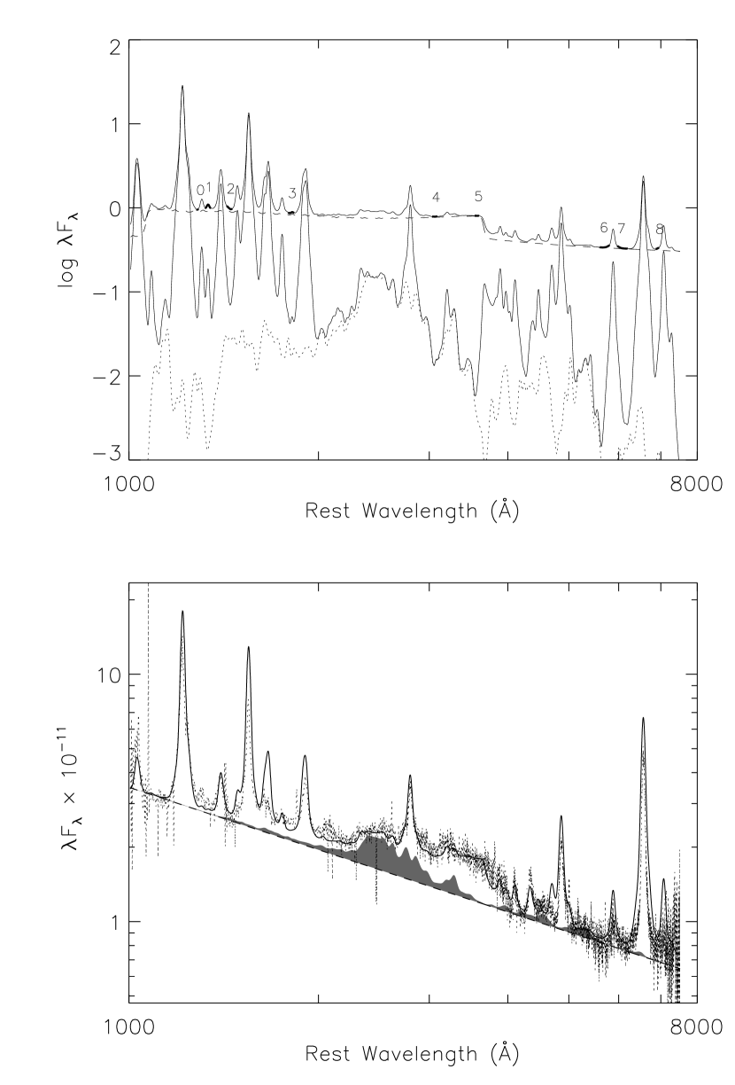
Figure 2: Upper panel: Model-A spectrum simulated for a single cloud with $\alpha(UV)$ = $-$0.2, $\Gamma$ = 2.8, $\alpha(OX)$ = $-$1.4, $T_{cut}$ = 1.5 $\times 10^{5}$ K, and $kT_{IR}$ = 0.136 eV, together with gas density of $N_{H}=10^{10}$ cm^-3, ionizing parameter of $U=10^{-1}$, microturbulence of $V_{turb}$ = 5 km s^-1, and the solar abundance. The spectrum by solid line on the top is the total flux of the model spectrum, while the spectrum by dashed line is the Balmer and Paschen continua. The spectrum by solid line in the middle is the total flux of all line emissions including Fe II, and the spectrum by dotted line is the contribution from Fe II emission alone. The numbers denotes the location of individual continuum windows (CWs; see Table 5). Lower panel: Model-B spectrum (solid line) compared with the observed spectrum of PG 1626+554 (dotted line). This model spectrum is made by applying the SMC-like intrinsic extinction of $E_{B-V}$ = 0.13 to the Model-A spectrum in the upper panel and adding a power-law continuum without extinction. Extinction, power-law index, and a covering factor of 0.5 are found as a result of adjustment to reproduce the observed spectrum of PG 1626+554. The power-law continuum is plotted by dashed line, and Fe II emission is shown by shaded areas.

where $\alpha(OX)=-\Gamma+1$, $\alpha(UV)$ = $-$0.9$-$+0.3, $\Gamma$ = 2.0$-$3.5, $T_{cut}$ = 1.5 $\times 10^{5}$ K, and $kT_{IR}$ = 0.136 eV. The coefficient $a$ is adjusted to produce the optical to the X-ray spectral index $\alpha(OX)=-1.4$. The incident continuum illuminates a single BELR cloud having the gas density of $N_{H}=10^{9}-10^{11}$ cm^-3, the ionizing parameter of $U=10^{-3}-10^{-0.5}$, the microturbulence of $V_{turb}$ = 0$-$10 km s^-1, and the solar abundance. Our calculations were performed for 810 sets of parameters with a grid of points, ($\alpha(UV)$, $\Gamma$, $N_{H}$, $U$, $V_{turb}$) = (3, 6, 3, 5, 3), where $\alpha(UV)$ = 3 means that the calculations were made for three different values of $\alpha(UV)$. An example of our synthetic spectra is shown in the upper panel of Figure 2 (hereafter called the model-A spectrum). After applying the internal SMC-like extinction of $E_{B-V}$ = 0.13, this spectrum reasonably reproduces the observed spectrum of PG 1626+554 as shown in the lower panel of Figure 2 (hereafter called the model-B spectrum). In the following, we use these single-cloud models. It should be noted that Baldwin et al. (2004) used the CLOUDY combined with the same 371-level Fe⁺ model as used in this paper, and introduced a microturbulence $V_{turb}>100$ km s^-1 to fit the observed UV Fe II feature. On the other hand, our model can reproduce the UV Fe II emission feature with a modest microturbulence of $V_{turb}=0-10$ km s^-1. This difference comes from the choice of the UV bump cutoff temperature $T_{cut}$; we used $T_{cut}=1.5\times 10^{5}$ K, while Baldwin et al. (2004) used a higher temperature 10⁶ K, causing the excessive reduction of the Fe II emissivity which then needs to be compensated by increasing microturbulence. Further discussion will exceed the scope of this paper, and will be given in a forthcoming paper.

The continuum windows are listed in Table 5 together with the range of the contribution from all emission lines to the total flux in 810 synthetic spectra. Note that we assumed the covering factor of 0.5. This factor was derived from the comparison between the observed spectrum of PG 1626$+$554 and the model-B spectrum presented in the lower panel in Figure 2. As shown in Table 5, there are no ideal continuum windows where the contribution of emission lines can be ignored. However, several good continuum windows exist in the wavelength region longward of 3000 Å where the contribution from all emission lines are only 1 or 2% of the total flux. In the wavelength region shortward of 1500 Å, the contribution from emission lines are relatively large at a level of 4$-$9%. Considering the importance of constraining the continuum levels in both sides of the Fe II emission features, we decided to use the continuum window of CW1 (1320$-$1350 Å) in addition to the other five windows of CW3, CW4, CW5, CW6, and CW7 in Table 5. Thus, a total of such six windows were used to fit the power-law and Balmer continua to the quasar spectrum.

3.2 Continuum Subtraction

The following procedure was used to subtract the continua from the quasar spectrum. First, the observed flux in the continuum window is decreased by taking into account the predicted contribution from non-continuum emission listed in column 4 of Table 5; for example, the total flux in CW1 is decreased by 7%. Then, the power-law and Balmer continua are simultaneously fitted to the fluxes thus decreased in the six continuum windows. Finally, the power-law and Balmer continua are subtracted from the original, observed spectrum, resulting in the continuum-subtracted spectrum consisting of line emission alone.

Our fitting models of the power-law and Balmer continua $F_{\nu}^{Cont}$ are in the form of

$$F_{\nu}^{Cont} = F_{0}[(\nu/\nu_{0})^{\alpha(UV)}+aF_{\nu}^{Bac}],$$ (2)

where $\nu_{0}$ is the frequency at 5700 Å and $F_{\nu}^{Bac}$ is the empirical distribution of Balmer continuum by Grandi (1982):

$$F_{\nu}^{Bac}=B_{\nu}(T_{e})(1-e^{-\tau_{\nu}})\quad\textrm{for}\quad\nu\geq\nu_{BE},$$ (3)

where $\tau_{\nu}=\tau_{BE}(\nu/\nu_{BE})^{-3}$, and $B_{\nu}(T_{e})$ is the Planck function at the electron temperature $T_{e}$. $\nu_{BE}$ and $\tau_{BE}$ are the frequency and optical depth at the Balmer edge at $\lambda$ = 3647 Å, respectively. Equation (2) has five fitting parameters, $F_{0}$, $\alpha$(UV), $a$, $T_{e}$, and $\tau_{BE}$.

The procedure of subtracting the continua is shown in Figure 3, plotting the spectra of I Zw 1 for two cases without and with correction for possible intrinsic extinction, namely, zero intrinsic extinction (left panels) and SMC-like intrinsic extinction of $E_{B-V}$ = 0.09 inferred from the O I line ratio (right panels). Note that the correction for Galactic extinction is applied to both cases. The top panels show the spectrum to which the model continua are fitted. The best-fit models are shown by the solid line for the power-law continuum and by the dashed line for the Balmer continuum. The middle and bottom panels show the power-law subtracted spectra in the UV and optical. The dashed line in the middle panels is the best-fit Balmer continuum. Note that the Balmer continuum is zero longward of the Balmer edge at 3647 Å. The spectra plotted in the middle and bottom panels are dominated by Fe II emission in the UV and optical except for the Balmer continuum, Mg II $\lambda 2798$, H$\gamma$, H$\beta$, [O III] $\lambda$$\lambda$4959,5007, and [Fe II] $\lambda$$\lambda$5158,5269 (see Figure 4).

The spectrum corrected for the intrinsic extinction (right panels) has the UV and optical Fe II fluxes and the Mg II line flux which are 1.59$-$2.09, 1.08$-$1.13, and 1.62 times greater than those deduced from the spectrum without intrinsic extinction (left panels), respectively. Thus, the line flux ratios, Fe II(UV)/Mg II and Fe II(opt)/Mg II, after corrected for the intrinsic extinction, are 0.98$-$1.29 and 0.67$-$0.70 times those without intrinsic extinction, respectively. It is therefore concluded that the error associated with the cases with and without intrinsic extinction is 30% at most in Fe II(UV, opt)/Mg II. This error is much smaller than that in the Balmer continuum flux; the flux corrected for the intrinsic extinction is almost eight times smaller than that without intrinsic extinction (see Table 8).

3.3 Template Fe II Spectrum and Removal of Non-Fe II Emission Lines

The UV and optical spectra of I Zw 1, after subtracting the power-law and Balmer continua and correcting for the Galactic extinction only, are plotted in Figure 4. The solid lines show the Fe II spectra, while the dotted lines show the contributions of Mg II $\lambda 2798$ and other optical emission lines such as H$\gamma$, H$\beta$, [O III] $\lambda$$\lambda$4959,5007, two [Fe II] lines and one Fe II] line which are blended near 5158 Å (Moore’s (1972) multiplet numbers of 18F $\lambda$5158, 19F $\lambda$5158, and 35 $\lambda$5161), and three [Fe II] lines blended near 5269 Å (19F $\lambda$5262 and 18F $\lambda$$\lambda$5269,5273). As shown in the left panel of Figure 5, the observed H$\alpha$ line profile is well fitted by two Gaussian components with different FWHMs of 690 and 2700 km s^-1 and the peak height ratio of 1:0.4. The 690 km s^-1 component is blueshifted relative to the 2700 km s^-1 component by 150 km s^-1. The broad component of Mg II $\lambda 2798$ with a FWHM of 5720 km s^-1 reported by Vestergaard & Wilkes (2001) has not been confirmed in our analysis of the H$\alpha$ profile. In the right panel of Figure 5, the H$\alpha$ template profile composed of these two components is compared with the spectrum centered at H$\beta$. Differences between the observed spectrum and the H$\alpha$ template could be mostly attributed to broad features of Fe II emission. The H$\alpha$ template is scaled in flux and shifted in wavelength to measure the contributions of the other broad emission lines, namely, H$\gamma$, H$\beta$, and Mg II $\lambda$2798. For the Balmer lines, H$\gamma$, and H$\beta$, the relative strength of the two Gaussian components was fixed to that (1:0.4 for the peak height ratio) of the H$\alpha$ profile, while for the Mg II $\lambda$2798 line, the relative strength is varied and determined to be 1:0.23 by fitting as described in the later paragraph in this sub-section. The H$\alpha$ template cannot be applied to the forbidden and semi-forbidden lines, namely, [O III] $\lambda$$\lambda$4959,5007, [Fe II], and Fe II]. The FWHM measurements of [O III] $\lambda$$\lambda$4959,5007 before subtracting the contribution of the Fe II emission, are 910 and 1360 km s^-1, respectively, and are broader than the real FWHM values due to broadening by the broad Fe II emission features. We therefore assumed the FWHM of the narrow component, 690 km s^-1, to be the FWHMs of these lines. The relative intensities of [O III] $\lambda$$\lambda$4959,5007 were assumed to be 1:3. For measuring the contributions of the [Fe II] and Fe II] lines, the line strengths relative to nearby Fe II emission were fixed to those measured by V$\acute{\textrm{e}}$ron-Cetty, Joly, & V$\acute{\textrm{e}}$ron (2004).

The subtractions of the forbidden and semi-forbidden lines may not be accurate due to the large uncertainties of their FWHMs. Nonetheless, the errors associated with the subtraction of these lines is estimated to be very small and can be ignored for the following reasons; (1) two Fe II templates covering two wavelength regions of 4400$-$4700 Å and 5100$-$5600 Å are used to measure the strengths of optical Fe II emission, and none of them cover the wavelengths of the [O III] lines, and (2) the contributions of the [Fe II] and Fe II] lines are very small when compared with the total strengths of the Fe II emission in 4400$-$4700 Å and 5100$-$5600 Å, i.e., 2$-$3% and 3$-$4%, respectively. It is noted that the wavelengths of H$\gamma$ and H$\beta$ are out of the range of optical templates.

Mg II $\lambda$2798 is the $3s^{2}S-3p^{2}P^{0}_{1/2,3/2}$ resonance doublet at 2795.5 and 2802.7 Å. This 2795.5/2802.7 doublet ratio changes from 2/1 to 1/1 for an entirely thermalized gas (Laor et al., 1997b). Because Mg II $\lambda$2798 heavily blends with Fe II emission lines, it is difficult to deduce the spectral feature of Fe II emission around Mg II $\lambda$2798 from the observed spectrum. The choice of the Fe II feature under the Mg II line profile would little alter the integrated flux of the broad Fe II feature. However, it can significantly affect the Mg II line flux. To determine the Fe II emission level obscured by the Mg II line profile, we take a semi-empirical approach with two assumptions: (1) Mg II $\lambda$2798 is purely made up with the $3s^{2}S-3p^{2}P^{0}_{1/2,3/2}$ resonance doublet, each of which has a line profile of the H$\alpha$ template, and (2) the spectral shape of Fe II is the same as that in the model spectrum shown in Figure 2.

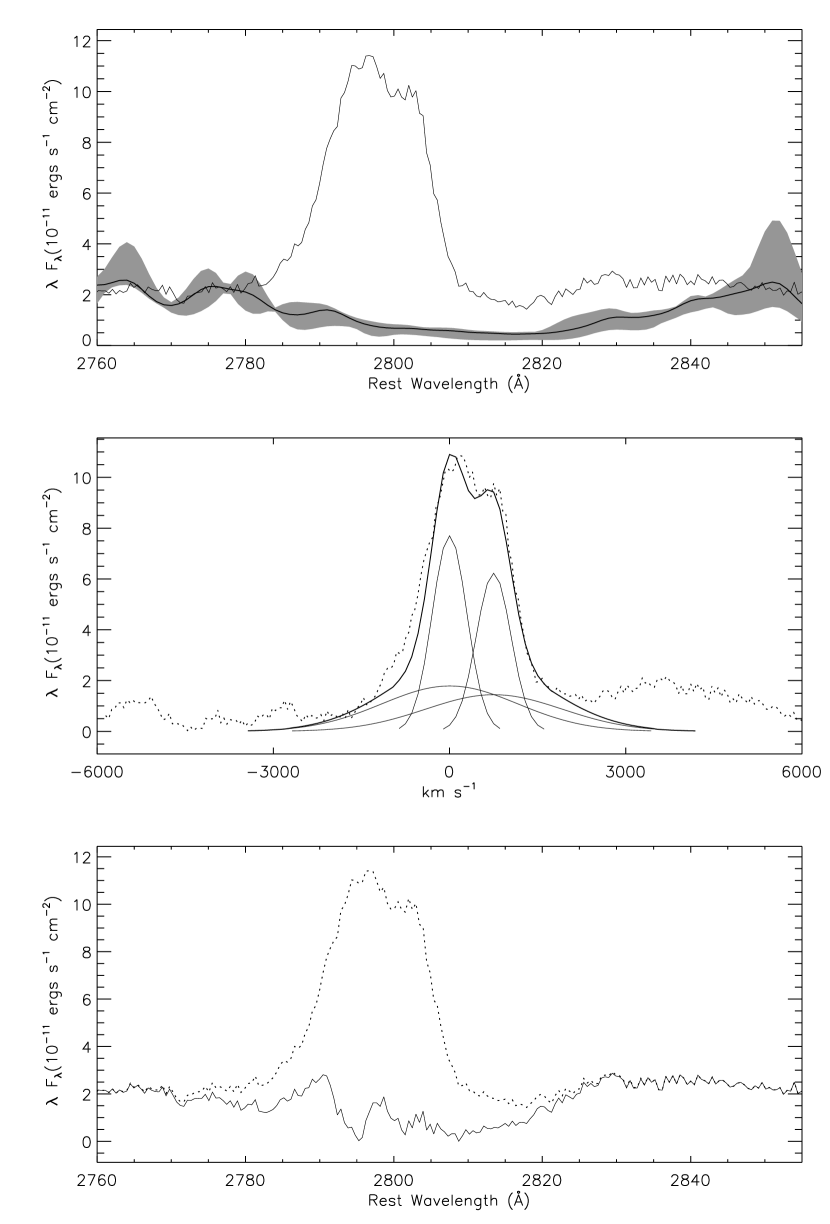
Figure 6: Top panel shows the Model-A spectrum (thick solid line) of Fe II emission overplotted on the I Zw 1 spectrum (thin solid line) around Mg II $\lambda$2798. The model spectrum was convolved with a 690 km s^-1FWHM profile. The shaded area is a range allowed by synthetic Fe II spectra in the parameter space used to study the continuum windows in section 3.1. The middle panel shows the Mg II $\lambda$2798 fit (thick solid line) to the spectrum (dotted line) where the model spectrum of Fe II has been subtracted. The Mg II $\lambda$2798 fit consists of doublet lines at 2795.5 and 2802.7 Å and each line has two Gaussian components (thin solid lines) with FWHMs of 690 and 2700 km s^-1 as in the case of the H$\alpha$ template. The intensity ratio of the doublet lines is 1.2:1 and the peak height ratio of two Gaussian components is 1:0.23 with no velocity difference between them. The bottom panel shows the spectrum (thin solid line) of Fe II emission overplotted on the I Zw 1 spectrum (dotted line). This Fe II spectrum was obtained by subtracting the Mg II $\lambda$2798 fit from the observed spectrum.

The model-A spectrum of Fe II emission around Mg II $\lambda$2798 is overplotted on the I Zw 1 spectrum in the top panel of Figure 6, after convolved with a 690 km s^-1 FWHM profile. The shaded area is a range allowed by synthetic Fe II spectra in the parameter space used to study the continuum windows in section 3.1, where the synthetic spectra are normalized at 2775 Å. To analyze the contribution of Mg II $\lambda$2798, the Fe II model-A spectrum was subtracted from the I Zw 1 spectrum and the resultant spectrum was fitted by the H$\alpha$ template with small modifications. Our Mg II $\lambda$2798 models purely consists of the resonance doublet, and each line of the doublet has a line profile of the H$\alpha$ template. The relative strength of the doublet, the peak height ratio of the Gaussian component, and the relative velocity of the 2700 km s^-1 component to the 690 km s^-1 component are set to be free parameters. The best fit is shown in the middle panel of Figure 6, for the case that the relative strength of the doublet is 1.2:1, the peak height ratio of the Gaussian component is 1:0.23, and the relative velocity between the 2700 and 690 km s^-1 components is zero. Our best fit is in good agreements with Laor et al. (1997b) who obtained 1.2:1 for relative doublet strengths by fitting the H$\alpha$ profile. When compared to Laor et al. (1997b), our fit is significantly improved especially over the both wings of the line profile with no need of a very broad 5720 km s^-1 component. This good fit would support our approach using model spectra to define the baseline of Mg II$\lambda$2798. The resultant semi-empirical Fe II template spectrum is overplotted on the I Zw 1 spectrum in the bottom panel of Figure 6. This template spectrum is the difference of I Zw 1 spectrum minus the fit of Mg II$\lambda$2798.

In our approach, the flux of Mg II $\lambda$2798 is the sum of the residual in the region of 2770$-$2830 Å after subtracting the Fe II template from the I Zw 1 spectrum. The flux of Mg II $\lambda$2798 thus measured is 61.1 $\times 10^{-14}$ ergs s^-1 cm^-2. If the baseline of Mg II $\lambda$2798 is a straight line between the minimum points at 2771 and 2818 Å, the Mg II flux becomes 10% smaller, while the baseline is defined by the minimum points allowed for our models, the flux becomes 8% greater. Thus, the choice of the baseline is associated with a 10% error in the Mg II flux, which should be regarded as a typical size of the systematic error. Our Mg II $\lambda$2798 flux is in between the other two values reported by Laor et al. (1997b) and Vestergaard & Wilkes (2001). The former is 52.1 $\times 10^{-14}$ ergs s^-1 cm^-2 (85 % of ours), and the latter is 94.3 $\times 10^{-14}$ ergs s^-1 cm^-2 (154 % of ours). Difference in the Mg II $\lambda$2798 flux between these authors is not very small, therefore a care is needed when comparing the fluxes taken from different sources.

Our Fe II template spectrum is compared with that by Vestergaard & Wilkes (2001) in the UV in the upper panel in Figure 7 and that by V$\acute{\textrm{e}}$ron-Cetty, Joly, & V$\acute{\textrm{e}}$ron (2004) in the optical in the lower panel, along with the model-A spectrum and the other synthetic spectrum. The template by Vestergaard & Wilkes (2001) and the two synthetic spectra are scaled in flux, in such a way that the integrated fluxes match with our template spectrum between 2200 and 3100 Å. Because the optical template by V$\acute{\textrm{e}}$ron-Cetty, Joly, & V$\acute{\textrm{e}}$ron (2004) is given in an arbitrary units, it is scaled to match with our template spectrum in 4400$-$4700 Å and 5100$-$5600 Å. As a result of flux-scaling, the original UV template spectrum by Vestergaard & Wilkes (2001) was multiplied by a factor of 1.4. The scaling of 1.4 in UV flux can mostly be attributed to the choice of the continuum level. They used a pure power-law continuum model to fit the I Zw 1 spectrum, and ignored the contribution from the Balmer continuum because their I Zw 1 spectrum does not cover wavelengths around the edge of the Balmer continuum which is used to measure the strength of the Balmer continuum. The power-law continuum fitting was made using the two continuum windows at 1675$-$1690 Å and 3007$-$3027 Å. As a result, their continuum level is significantly higher than ours as can be seen in the left panels of Figure 3, which in turn decreases their Fe II flux. The magnification by a factor of 1.4 makes their template spectrum more spiky than ours. Nonetheless, there is a good agreement between the two template spectra except in the region around 2800 Å. In the optical, there is a good agreement between the two template spectra except in the region around 4900 Å. The disagreement around 4900 Å may be caused by their H$\beta$ $\lambda$4861 profile. V$\acute{\textrm{e}}$ron-Cetty, Joly, & V$\acute{\textrm{e}}$ron (2004) fitted H$\beta$ using the line profile comprised of a Lorentzian component with a FWHM of 1100 km s^-1 and Gaussian component with a FWHM of 5600 km s^-1. As already discussed and shown in Figure 5, such a very broad component with a FWHM of 5600 km s^-1 is not confirmed in our analysis of the H$\alpha$ profile.

Two synthetic spectra in the framework of photoionization are compared with observations; one is based on model-A and the other is a spectrum in a low-density cloud. The synthetic spectra were convolved with a line profile of a FWHM of 1660 km s^-1 that is the FWHM of Mg II $\lambda$2798 in the single Gaussian form as discussed in footnote 7. As discussed in section 3, model-A is used to specify the contributions of emission lines to the spectra of normal quasars and has $N_{H}=10^{10}$ cm^-3 with $U=10^{-1}$ and $V_{turb}$ = 5 km s^-1. The low-density cloud model has $N_{H}=10^{7}$ cm^-3 with $U=10^{-2}$ and $V_{turb}$ = 0 km s^-1 with other parameters identical to model-A. It is generally considered that Fe II emission arises in BELR clouds with a high gas density of $N_{H}\geq 10^{9.5}$ cm^-3 (e.g., Verner et al. 1999; Sigut & Pradhan 2003). In this sense, model-A is more conventional than the low-density cloud (LDC) model. Compared to the template spectrum, the model-A spectrum has an excess in flux around 2400 Å while a deficiency longward of 2900 Å. In the optical, the model-A spectrum fails to produce the Fe II emission by a factor of 10. This is a major reason that a non radiative heating mechanism, such as a shock model (e.g. Collin & Joly 2000), is considered to be necessary to account for strong optical Fe II emitters like I Zw 1. However, it is interesting that the LDC model reproduces the strong optical Fe II emission, although there is a severe deficiency around 4600 Å. Further investigation is required if photoionization can reproduce the strong optical Fe II emission.

4 Application of the Fe II Template Spectrum

4.1 Fitting to Quasar Spectra

To apply the Fe II template spectrum obtained from the NLSy1 I Zw 1 to other quasars, broadening of the template spectrum is needed to match with the line width of the quasar spectrum in consideration. We use the similar broadening method used by Boroson & Green (1992) and Vestergaard & Wilkes (2001); broadening the template using a relation,

$$\textrm{FWHM}(\textrm{QSO})^{2} = \textrm{FWHM}(\textrm{convolution})^{2}+\textrm{FWHM}(\textrm{I Zw 1})^{2},$$ (4)

where FWHM(QSO), FWHM(I Zw 1), and FWHM(convolution) are used to represent the line width of the target quasar, that of I Zw 1, and the width of additional convolution applied to the I Zw 1 spectrum (i.e., broadening). The actual sequence of broadening would perform as follows: (a) the FWHM of Mg II is measured in the original spectrum containing the Fe II emission features; (b) this initial FWHM value is used to broaden the I Zw 1 template spectrum; (c) the broadened template is used to subtract the Fe II emission features from the original spectrum; (d) the final FWHM value is determined by fitting a single Gaussian component to the Fe II-subtracted spectrum; (e) the final FWHM value is used to broaden the I Zw 1 template spectrum, and the Fe II emission strengths is re-measured for the final results. According to our experience, using the initial FWHM value of Mg II is good enough to have accurate strengths of the Mg II and Fe II emission lines; the Mg II and Fe II fluxes measured using the initial FWHM value differ only $<$ 1% typically or 3% at most from those measured using the final FWHM value.

If the I Zw 1 spectrum is similar to those of other quasars, the Fe II template spectrum could be fitted well simultaneously from the UV to the optical, using a single scaling in flux. However, I Zw 1 is a peculiar quasar as classified NLSy1 with extremely strong Fe II emission, and the shape of the Fe II spectrum would differ from other quasars. To flexibly cope with the possible variety of Fe II spectrum shapes from quasar to quasar, we subdivide the template spectrum into five segments, and allow five separate flux-scalings for template fitting, i.e., one independent flux-scaling for each template segment. As shown by thick lines in Figure 4, these segments correspond to the wavelength bands called $U1$ (2200$-$2660 Å), $U2$ (2660$-$3000 Å), $U3$ (3000$-$3500 Å), $O1$ (4400$-$4700 Å), and $O2$ (5100$-$5600 Å). Fitting of the Fe II emission is only performed within these bands. The fitting function of our Fe II emission models is of the form:

$$F_{\nu}^{Fe} = \ \ \ F_{\nu}^{Fe}(U1)+b_{1}F_{\nu}^{Fe}(U2)+b_{2}F_{\nu}^{Fe}(U3)$$ (5)

$$+ b_{3}F_{\nu}^{Fe}(O1)+b_{4}F_{\nu}^{Fe}(O2),$$

where $F_{\nu}^{Fe}(X)$ is the Fe II template spectrum segment for the wavelength band of $X=U1,U2,..,O2$. The coefficients $b_{i}$ are the flux-scaling parameters used to measure the relative strength of the Fe II emission in the corresponding wavelength band.

The model spectrum consisting of the power-law and Balmer continua and the Fe II emission is therefore given by

$$F_{\nu} = F_{0}[(\nu/\nu_{0})^{\alpha(UV)}+aF_{\nu}^{Bac}+bF_{\nu}^{Fe}].$$ (6)

The best-fit models of this form are compared with the original spectra of 14 quasars in Figure 8. All the original spectra have been corrected for the Galactic extinction. The panels are sorted by $M_{B}$ with the lowest luminosity at the top. For two quasars with red spectral index, I Zw 1 and PG 1114+445, an alternative case is also shown such that the intrinsic SMC-like extinction of $E_{B-V}$ = 0.09 has been applied together with the Galactic extinction. The fits are summarized in Table 6.

The lines of H$\beta$, H$\gamma$, and [O III] as well as Mg II were measured by fitting a Gaussian after subtracting the best-fit Fe II emission model. It is noted that fitting was not performed in 4200$-$4400 Å and 4700$-$5100 Å where H$\beta$, H$\gamma$, and [O III] are located. Instead, it is assumed that the spectra of 4200$-$4400 Å and 4700$-$5100 Å have the same strength as $b_{3}F_{\nu}^{Fe}(O1)$ and $b_{4}F_{\nu}^{Fe}(O2)$, respectively, at their boundaries. Fluxes of lines shortward of 2000 Å were measured by fitting a Gaussian to the continuum-subtracted spectrum. Table 7 lists the FWHMs of Mg II, H$\alpha$, and [O III], and the ratios between the flux of Mg II and H$\alpha$ measured by fitting the two Gaussian components and that by fitting a single Gaussian component. Tables 8 lists the fluxes of emission lines and the Balmer continuum as well as the flux at 1450 Å. It should be kept in mind that the cases with and without intrinsic extinction can alter the line ratios significantly; for example, the correction for the intrinsic SMC-like extinction of $E_{B-V}$ = 0.09 increases the Fe II($U1$)/Mg II ratio by a factor of 1.3 and decreases Fe II($O1$)/Fe II($U1$) by a factor of two. Furthermore, the Balmer continuum flux is decreased by a factor of eight.

4.2 Comparison with Previous Work

We start with relating our Fe II bands to those previously used in the literature. Optical Fe II line emission, especially Fe II $\lambda$4570 and $\lambda$5250 (referred to by Phillips (1978) as the $\lambda$5190,5320 blend) has been observed in many quasars (e.g., Boroson & Green 1992; Sulentic, Marziani, & Dultzin-Hacyan 2000). Fe II $\lambda$4570 is a blend of multiplets 37, 38, and 43 in the wavelength range between H$\gamma$ and H$\beta$, and Fe II $\lambda$5250 is a blend of multiplets 42, 48, 49, and 55 in the wavelength range of 5100$-$5600 Å (Phillips, 1978). In fact, the integrated Fe II flux $F(O1)$ in the $O1$ band and similarly $F(O2)$ in the $O2$ band are equivalent to the integrated fluxes usually used such as

$$F(\textrm{Fe II }\lambda 4570) = F(O1)$$

$$F(\textrm{Fe II }\lambda 5250) = F(O2).$$ (7)

Prior to this work, the largest sample of quasar spectra with Fe II emission observed both in the UV and optical is given by Wills, Netzer, & Wills (1985). They analyzed seven low-redshift quasars with a wide wavelength coverage from 1800 to 5500 Å, and measured the Mg II flux and the integrated Fe II fluxes in 2000$-$3000 Å, 3000$-$3500 Å, and 3500$-$6000 Å. Two quasars in their sample, QSO 0742+318 and 3C 273, are commonly included in our sample. Because our Fe II bands are different from theirs, transformation equations between the two different systems are needed. Figure 9 shows the cumulative Fe II flux as a function of wavelength, derived from the best-fit Fe II templates for I Zw 1 and PG 1626+554. We then find the following transformation equations:

$$F(2000-3000\hskip 2.84526pt\mbox{\AA}) = 1.064(\pm 0.005)\times[F(U1)+F(U2)]$$

$$F(3000-3500\hskip 2.84526pt\mbox{\AA}) = F(U3)$$

$$F(3500-6000\hskip 2.84526pt\mbox{\AA}) = 1.997(\pm 0.001)\times[F(O1)+F(O2)],$$

where $F(X)$ are the integrated Fe II fluxes in the wavelength range or band $X$.

The measurements of various emission fluxes in QSO 0742+318 and 3C273 by Wills, Netzer, & Wills (1985) are compared with our measurements in Table 9. No correction for the intrinsic extinction was made in both measurements. While their optical line strengths agree well with ours within an accuracy of 20%, those of UV lines shortward of 3000 Å and the Balmer continuum largely differ from each other and the difference is as large as a factor of 2 to 3. The reason for such a large difference is not clear, but may possibly be because (1) the International Ultraviolet Explorer UV spectra used by Wills, Netzer, & Wills (1985) are not so good as expected, and/or because (2) the UV continuum levels estimated by Wills, Netzer, & Wills (1985) are poorly determined due to their limited wavelength coverage in the UV. In fact, their UV continuum levels are 10% smaller than ours, which increases their Fe II(2000$-$3000 Å) strengths by this factor when compared to ours.

5 Correlations of Fe II emission with other spectral properties

Large observational efforts have been devoted to searching for correlations between Fe II emission and other spectral properties. Such correlation studies were mostly made against Fe II $\lambda$4570, which is practically identical to our Fe II ($O1$). This work should therefore be regarded as extension of previous studies by including UV Fe II emission. In the following, we simply show various correlations, although their statistical significance is limited because of our sample consisting of only 14 quasars. The non-abundance effects in the Fe II/Mg II flux ratio and related physical processes in BELR clouds will be discussed in a forthcoming paper.

Various $X$ versus $Y$ diagrams are shown in Figure 10, which are useful to study the non-abundance effects in Fe II emission. Regression analysis was performed to derive a linear relation ($Y=A+BX$), weighted by individual standard deviations of two variables $X$ and $Y$. The results are summarized in Table 10, showing the panel name identifying the diagram in Figure 10, the variables $X$ and $Y$, the sample number $N$, the intercept $A$, and the slope $B$, the linear-correlation coefficient $r$, and the confidence level.

There are well-known correlations, namely, larger Fe II ($O1$)/H$\beta$ for larger soft X-ray photon index $\Gamma$ (Wang, Brinkmann, & Bergeron, 1996; Lawrence et al., 1997; Laor et al., 1997a), for smaller FWHM of permitted lines (Zheng & O’Brien, 1990; Zheng & Keel, 1991; Lawrence et al., 1997), and for weaker [O III]/H$\beta$ (Boroson & Green, 1992). It is expected that these correlations are also seen for Fe II ($O1$)/Mg II, because both H$\beta$ and Mg II are collisionally excited in the partially ionized region in the BELR clouds (Kwan & Krolik, 1981). In fact, these correlations in our diagrams give a confidence level of (panel $g$) 97.9%, (panel $k$) 99.3%, and (panel $s$) 94.2%, respectively.

As shown in Table 10, there are eight correlations with a confidence level of 99% or higher, i.e., (1) (panel $a$) larger Mg II FWHM for larger H$\alpha$ FWHM, (2) (panel $e$) larger $\Gamma$ for fainter $M_{B}$, (3) (panel $i$) smaller Mg II FWHM for larger $\Gamma$, (4) (panel $k$) larger Mg II FWHM for smaller Fe II($O1$)/Mg II, (5) (panel $m$) larger black hole mass $M_{BH}$ for smaller $\Gamma$, (6) (panel $o$) larger $M_{BH}$ for smaller Fe II($O1$)/Mg II, (7) (panel $q$) larger [O III]/H$\beta$ for larger Mg II FWHM, and (8) (panel $x$) larger Fe II($O1$)/Mg II for larger Fe II($O1$)/Fe II($U1$). We note that the correlation of smaller Mg II FWHM for larger $\Gamma$ in panel $i$ is consistent with the correlation of smaller H$\beta$ FWHM for larger $\Gamma$ (Wang, Brinkmann, & Bergeron, 1996; Lawrence et al., 1997; Laor et al., 1997a).

The fact that six of eight correlations with a confidence level of 99% or higher are related to FWHM or $M_{BH}$ ($\propto$ FWHM²) may imply that $M_{BH}$ is a fundamental quantity that controls $\Gamma$ or SED of the incident continuum, which in turn controls the Fe II emission. Panel $m$ indicates that AGNs with smaller $M_{BH}$ have larger excess of soft X-rays, resulting in stronger Fe II emission, especially in the optical as shown in panel $n$ and $o$. This may agree with the result obtained for I Zw 1, because NLSy1s are a class of AGNs that harbor a low-mass BH at the center radiating near the Eddington limit (e.g., Boroson 2002). It is also interesting that the optical Fe II emission correlates better with other parameters than UV Fe II emission and that Fe II($O1$)/Fe II($U1$) tightly correlates with Fe II($O1$)/Mg II, but not with Fe II($U1$)/Mg II. These may indicate that UV and optical Fe II emission are generated in different regions of BELR clouds. The correlation of larger Mg II FWHM for brighter $M_{B}$ is consistent with a weak trend of larger FWHM of Balmer lines for higher luminosity found by various authors (e.g., Shuder 1984; Wandel & Yahil 1985; Kaspi et al. 2000).

Note that the results of linear regression analysis presented here were derived from the spectra with no correction for the intrinsic extinction. To evaluate the effect of intrinsic extinction, we analyzed the spectra of two quasars, PG 1114$+$445 and I Zw 1, with correction for the SMC-type extinction. The resulting change of confidence level is only within 4%, except for the result in panel $c$ and $d$ where the confidence level is decreased from 85% to 62% and increased from 18% to 97%, respectively. This is attributed to the difference in the Balmer continuum flux of I Zw 1, e.g., Bac/H$\beta$ is 23.4 (without intrinsic extinction) or 2.3 (with intrinsic extinction).

6 Summary

We have presented the spectra of 14 quasars with a wide wavelength coverage from 1000 to 7300 Å in the rest frame. The redshift ranges from $z=$ 0.061 to 0.555 and the luminosity from $M_{B}$ = $-$22.69 to $-$26.32. These spectra are in high quality and resulted from combining HST spectra with those taken on ground-based telescopes. We described the procedure of deriving the template spectrum of Fe II from the I Zw 1 spectrum, covering two wavelength regions of 2200$-$3500 Å and 4200$-$5600 Å where prominent Fe II emission is seen. Our Fe II template spectrum is semi-empirical in the sense that the synthetic spectrum calculated with the CLOUDY photoionization code is used to separate the Fe II emission from the Mg II $\lambda$2798 line.

Our procedure of measuring strengths of Fe II emission is twofold; (1) subtracting the continuum component by fitting models of the power-law and Balmer continua to the continuum windows which are relatively free from line emissions, and (2) fitting models of the Fe II emission made by the Fe II template to the continuum-subtracted spectra. From 14 quasars including I Zw 1, we obtained the Fe II fluxes in five wavelength bands from the UV to optical, the total flux of Balmer continuum, the flux and FWHM of Mg II $\lambda$2798, H$\alpha$, and other emission lines.

Regression analysis was performed to derive a linear relation between two variables ($Y=A+BX$), and eight correlations with a confidence level of 99% or higher were found. These are the correlations of (1) larger Mg II FWHM for larger H$\alpha$ FWHM, (2) larger $\Gamma$ for fainter $M_{B}$, (3) smaller Mg II FWHM for larger $\Gamma$, (4) larger Mg II FWHM for smaller Fe II($O1$)/Mg II, (5) larger $M_{BH}$ for smaller $\Gamma$, (6) larger $M_{BH}$ for smaller Fe II($O1$)/Mg II, (7) larger [O III]/H$\beta$ for larger Mg II FWHM, and (8) larger Fe II($O1$)/Mg II for larger Fe II($O1$)/Fe II($U1$). Six of these eight correlations are related to FWHM or $M_{BH}$ ($\propto$ FWHM²). This fact may imply that $M_{BH}$ is a fundamental quantity that controls $\Gamma$ or equivalently SED of the incident continuum that eventually controls Fe II emission.

Figure 1 and the Fe II template are available from the web site:
http://www.ioa.s.u-tokyo.ac.jp/^∼kkawara/quasars/index.html.

Table 1: Quasar Sample

Quasar	$\alpha$ (J2000.0)	$\delta$ (J2000.0)	Redshift	$M_{B}$	$E_{B-V}$
I Zw 1	00 53 34.9	+12 41 36	0.061	$-$22.97	0.06
QSO 0742+318	07 45 41.7	+31 42 56	0.462	$-$25.76	0.06
PG 0947+396	09 50 48.4	+39 26 51	0.206	$-$23.56	0.01
PG 1114+445	11 17 06.3	+44 13 34	0.144	$-$23.22	0.01
PG 1115+407	11 18 30.4	+40 25 55	0.154	$-$22.83	0.02
3C 273	12 29 06.6	+02 03 08	0.158	$-$26.13	0.02
3C 277.1	12 52 26.4	+56 34 19	0.320	$-$23.22	0.01
PG 1309+355	13 12 17.7	+35 15 23	0.184	$-$24.02	0.01
PG 1322+659	13 23 49.6	+65 41 48	0.168	$-$23.24	0.02
PG 1352+183	13 54 35.6	+18 05 18	0.152	$-$22.69	0.02
3C 323.1	15 47 43.6	+20 52 16	0.266	$-$24.33	0.05
3C 334.0	16 20 21.8	+17 36 23	0.555	$-$26.32	0.05
PG 1626+554	16 27 56.2	+55 22 32	0.132	$-$22.97	0.01
B2 2201+31A	22 03 14.9	+31 45 38	0.298	$-$25.60	0.12

Table 2: HST Observations

Quasars	$\lambda$ range	Grating	$t_{int}^{a}$	Date
	(Å)		(sec)
I Zw 1	1140$-$1606	FOS G130H	29880.0	1994 Feb 13
	1590$-$2312	FOS G190H	6120.0	1994 Sep 14
	2222$-$3277	FOS G270H	2160.0	1994 Sep 14
QSO 0742+318	1590$-$2312	FOS G190H	4483.9	1994 Mar 14
	2222$-$3277	FOS G270H	1598.5	1994 Mar 14
PG 0947+396	1140$-$1606	FOS G130H	4007.0	1997 May 06
	1590$-$2312	FOS G190H	1260.0	1997 May 06
	2222$-$3277	FOS G270H	450.0	1997 May 06
	3235$-$4781	FOS G400H	210.0	1997 May 06
PG 1114+445	1140$-$1606	FOS G130H	9269.8	1996 Mar 13
	1590$-$2312	FOS G190H	1560.0	1996 Mar 13
	2222$-$3277	FOS G270H	160.0	1996 Mar 13
	3235$-$4781	FOS G400H	120.0	1996 Mar 13
PG 1115+407	1140$-$1606	FOS G130H	3749.9	1996 Mar 19
	1590$-$2312	FOS G190H	760.0	1996 Mar 19
	2222$-$3277	FOS G270H	191.0	1996 Mar 19
	3235$-$4781	FOS G400H	154.0	1996 Mar 19
	4569$-$6818	FOS G570H	471.0	1996 Mar 19
3C 273	1140$-$1606	FOS G130H	7600.0	1991 Feb 17
	1590$-$2312	FOS G190H	5414.4	1991 Feb 14, 15
	2222$-$3277	FOS G270H	5414.4	1991 Feb 15
	2900$-$5700	STIS G430L	974.0	2002 Feb 01
	5240$-$10270	STIS G750L	776.0	2002 Feb 01
3C 277.1	1590$-$2312	FOS G190H	1986.0	1993 Jul 01
	2222$-$3277	FOS G270H	1122.0	1993 Jul 01
	3235$-$4781	FOS G400H	864.0	1993 Jul 01
	2900$-$5700	STIS G430L	2800.0	1999 Oct 12
	5240$-$10270	STIS G750L	2340.0	1999 Oct 11
PG 1309+355	1140$-$1606	FOS G130H	4580.0	1997 May 20
	1590$-$2312	FOS G190H	799.0	1997 May 20
	2222$-$3277	FOS G270H	306.0	1997 May 20
	3235$-$4781	FOS G400H	112.0	1997 May 20
PG 1322+659	1140$-$1606	FOS G130H	22147.6	1997 Jan 19
	1590$-$2312	FOS G190H	2549.9	1997 Jan 19
	2222$-$3277	FOS G270H	416.0	1997 Jan 19
	3235$-$4781	FOS G400H	334.0	1997 Jan 19
PG 1352+183	1140$-$1606	FOS G130H	2170.0	1996 Mar 26
	1590$-$2312	FOS G190H	702.0	1996 Mar 26
	2222$-$3277	FOS G270H	200.0	1996 Mar 26
	3235$-$4781	FOS G400H	156.0	1996 Mar 26
3C 323.1	1140$-$1606	FOS G130H	2310	1993 Jul 01
	1590$-$2312	FOS G190H	384.0	1993 Jul 01
	2222$-$3277	FOS G270H	225.0	1993 Jul 01
	3235$-$4781	FOS G400H	156.0	1993 Jul 01
3C 334.0	1590$-$2312	FOS G190H	648.0	1993 Jul 01
	2222$-$3277	FOS G270H	345.0	1993 Jul 01
	3235$-$4781	FOS G400H	252.0	1993 Jul 01
PG 1626+554	1140$-$1606	FOS G130H	3192.9	1996 Nov 19
	1590$-$2312	FOS G190H	654.0	1996 Nov 19
	2222$-$3277	FOS G270H	120.0	1996 Nov 19
	3235$-$4781	FOS G400H	92.0	1996 Nov 19
	4569$-$6818	FOS G570H	255.0	1996 Nov 19
	6270$-$8500	FOS G780H	825.0	1996 Nov 19
B2 2201+31A	1140$-$1606	FOS G130H	2790.0	1993 Jul 01
	1590$-$2312	FOS G190H	1104.0	1993 Jul 01
	2222$-$3277	FOS G270H	222.0	1993 Jul 01
	3235$-$4781	FOS G400H	132.0	1993 Jul 01

Table 3: Ground-Based Observations

Quasars	$\lambda$ range	$\Delta\lambda$	Spectrograph	$t_{int}$	Date	References
	(Å)	(Å)		(sec)
I Zw 1	3183$-$4073	1.2	KPNO 2.1m Goldcam		1995 Sep 22	Laor et al. (1997b)
	4008$-$7172	3.1	INT 2.5m IDS	1220	1987 Aug 15	ING archive
QSO 0742+318	2519$-$8510	2.47	McDonald 2.7m UVITS			Wills, Netzer, & Wills (1985)
PG 0947+396	4330$-$9225	2.47	KPNO 2.1m Goldcam	1680	2001 May 2,3	This work
PG 1114+445	4330$-$9226	2.47	KPNO 2.1m Goldcam	660	2001 May 2,3	This work
PG 1309+355	4331$-$9226	2.47	KPNO 2.1m Goldcam	420	2001 May 2,3	This work
PG 1322+659	4331$-$9226	2.47	KPNO 2.1m Goldcam	540	2001 May 2,3	This work
PG 1352+183	4329$-$9228	2.47	KPNO 2.1m Goldcam	540	2001 May 2,3	This work
3C 323.1	4331$-$9228	2.47	KPNO 2.1m Goldcam	1620	2001 May 2,3	This work
3C 334.0	4334$-$9225	2.47	KPNO 2.1m Goldcam	1080	2001 May 2	This work
	8700$-$13900	5.83	Subaru 8.2m CISCO	600	2001 May 9	This work
B2 2201+31A	4472$-$9488	2.47	KPNO 2.1m Goldcam	5400	1994 Sep 28	Corbin (1997)

Table 4: Multi-Wavelength Properties

Quasars	$B$	$B-V$	$\alpha$	$L_{60\mu m}/L_{V}$	$\Gamma$	Radio
I Zw 1	14.28	0.318	$-$1.19	2.12	3.05 $\pm$ 0.14	Q
QSO 0742+318	16.26	0.279	$-$0.73		1.56${}^{+0.52}_{-0.68}$	L
PG 0947+396	16.21	$-$0.043	$-$0.06	1.53	2.12 $\pm$ 0.30	Q
PG 1114+445	15.82	0.102	$-$1.04	0.89	2.13${}^{+0.24}_{-0.31}$	Q
PG 1115+407	16.25	0.021	0.05	$<$1.0	2.77 $\pm$ 0.17	Q
3C 273	13.01	0.108	$-$0.14	0.62	2.11 $\pm$ 0.01	L
3C 277.1	17.71	0.025	$-$0.24	1.43	2.59 $\pm$ 0.04	L
PG 1309+355	15.66	0.206	$-$0.63	$<$0.51	2.51 $\pm$ 0.07	Q
PG 1322+659	16.13	0.030	$-$0.20	0.60	2.97 $\pm$ 0.13	Q
PG 1352+183	16.33	0.026	$-$0.07	1.58	2.53 $\pm$ 0.26	Q
3C 323.1	16.19	$-$0.128	$-$0.21	0.40	2.43 $\pm$ 0.03	L
3C 334.0	16.30	$-$0.121	0.15	0.75	2.10 $\pm$ 0.08	L
PG 1626+554	15.75	$-$0.011	$-$0.20	0.34	2.61 $\pm$ 0.41	Q
B2 2201+31A	15.03	$-$0.085	$-$0.09		2.22${}^{+0.29}_{-0.31}$	L

Note. — Column 2: $B$ magnitudes derived from our spectra after corrected for the Galactic extinction given in Table 1. Column 3: Same as column 2 but for $B-V$. Column 4: Power-law index, $F_{\nu}\propto\nu^{\alpha}$, derived from our de-reddened continuum spectra. Fitting procedure is described in section 3.2. Column 5: The 60 $\mu$m luminosity relative to the optical V-band, as defined by $L_{60\mu m}/L_{V}=\nu_{60\mu m}F_{60\mu m}/\nu_{V}F_{V}$. The 60 $\mu$m data are taken from Sanders et al. (1989), van Bemmel, Barthel, & de Graauw (2000), and Haas et al. (2003). Column 6: X-ray photon index $\Gamma$ taken from Brinkmann, Yuan, & Siebert (1997) and Yuan et al. (1998). $\Gamma$ is defined by the power-law fit, i.e., $P_{E}$(photons s^-1 keV^-1) $\propto$ $e^{-N_{H}\sigma_{E}}$ $\times$ $E^{-\Gamma}$, where $N_{H}\sigma_{E}$ is the Galactic absorption. Column 7: Radio properties, namely, “Q” for radio-quiet and “L” for radio-loud, based on the 5 or 1.4 GHz flux in the FIRST catalog by Becker, White, & Helfand (1995), Kellermann et al. (1989), and Kuehr et al. (1981).

Table 5: Emission Line Contributions in Continuum Windows

Name	$\lambda$ range	$F_{\lambda}$(lines)/$F_{\lambda}$(total)	Adopted
	(Å)	(%)	(%)
CW0	1280$-$1290	4$-$9
CW1	1320$-$1350	5$-$8	7
CW2	1430$-$1460	6$-$9
CW3	1790$-$1830	2$-$5	4
CW4	3030$-$3090	1$-$2	1
CW5	3540$-$3600	1	1
CW6	5600$-$5800	2$-$3	3
CW7	5970$-$6200	2$-$3	3
CW8	6870$-$6950	7$-$8

Note. — Fractional contributions from all emission lines to the total flux of synthetic spectra. Column 3 gives the values expressed in percentage, based on our single cloud models calculated for 810 grids in the parameter space. Column 4 gives the values adopted for our use of continuum subtraction.

Table 6: Parameters for Fitting

	Power-law continuum			Balmer continuum				Fe II emission
Quasars	$F_{0}$	$\alpha$(UV)		$T_{e}$ (104K)	$\tau_{BE}$	$h_{BE}$		$b$	$b_{1}$	$b_{2}$	$b_{3}$	$b_{4}$
With no intrinsic extinction
PG 1352+183	1.076 $\pm$ 0.106	$-$0.07 $\pm$ 0.02		2.69 $\pm$ 0.13	0.75 $\pm$ 0.04	1.41 $\pm$ 0.17		0.0361 $\pm$ 0.0017	0.92 $\pm$ 0.06	0.52 $\pm$ 0.04	0.37 $\pm$ 0.02	0.12 $\pm$ 0.01
PG 1115+407	1.207 $\pm$ 0.184	0.05 $\pm$ 0.04		1.85 $\pm$ 0.09	1.29 $\pm$ 0.06	0.82 $\pm$ 0.15		0.0340 $\pm$ 0.0021	0.87 $\pm$ 0.07	0.67 $\pm$ 0.06	0.44 $\pm$ 0.02	0.21 $\pm$ 0.02
PG 1626+554	1.995 $\pm$ 0.279	$-$0.20 $\pm$ 0.00		3.43 $\pm$ 0.17	1.05 $\pm$ 0.05	1.50 $\pm$ 0.24		0.0148 $\pm$ 0.0013	1.17 $\pm$ 0.10	0.78 $\pm$ 0.08	0.52 $\pm$ 0.02	0.26 $\pm$ 0.03
I Zw 1	10.55 $\pm$ 0.64	$-$1.19 $\pm$ 0.00		1.56 $\pm$ 0.00	10.1 $\pm$ 0.0	0.70 $\pm$ 0.05		0.0958 $\pm$ 0.0003	1.00 $\pm$ 0.00	1.00 $\pm$ 0.01	0.98 $\pm$ 0.01	1.01 $\pm$ 0.01
PG 1114+445	1.904 $\pm$ 0.106	$-$1.04 $\pm$ 0.00		2.24 $\pm$ 0.06	1.45 $\pm$ 0.06	1.94 $\pm$ 0.11		0.0138 $\pm$ 0.0008	0.98 $\pm$ 0.08	0.79 $\pm$ 0.07	1.07 $\pm$ 0.02	0.42 $\pm$ 0.02
3C 277.1	0.359 $\pm$ 0.015	$-$0.24 $\pm$ 0.01		1.78 $\pm$ 0.04	0.19 $\pm$ 0.01	1.24 $\pm$ 0.05		0.0358 $\pm$ 0.0013	0.66 $\pm$ 0.04	0.44 $\pm$ 0.03	0.23 $\pm$ 0.01	0.14 $\pm$ 0.01
PG 1322+659	1.111 $\pm$ 0.142	$-$0.20 $\pm$ 0.02		1.83 $\pm$ 0.00	0.20 $\pm$ 0.01	1.96 $\pm$ 0.29		0.0288 $\pm$ 0.0013	0.91 $\pm$ 0.05	0.61 $\pm$ 0.04	1.05 $\pm$ 0.02	0.42 $\pm$ 0.02
PG 0947+396	1.233 $\pm$ 0.061	$-$0.06 $\pm$ 0.00		1.19 $\pm$ 0.06	1.11 $\pm$ 0.06	1.27 $\pm$ 0.07		0.0344 $\pm$ 0.0008	0.82 $\pm$ 0.04	0.44 $\pm$ 0.03	0.31 $\pm$ 0.01	0.10 $\pm$ 0.01
PG 1309+355	2.551 $\pm$ 0.183	$-$0.63 $\pm$ 0.02		3.73 $\pm$ 0.19	0.47 $\pm$ 0.02	1.12 $\pm$ 0.09		0.0249 $\pm$ 0.0008	0.84 $\pm$ 0.05	0.33 $\pm$ 0.05	0.82 $\pm$ 0.02	0.42 $\pm$ 0.02
3C 323.1	1.330 $\pm$ 0.077	$-$0.21 $\pm$ 0.02		1.92 $\pm$ 0.00	0.02 $\pm$ 0.00	1.51 $\pm$ 0.09		0.0215 $\pm$ 0.0010	0.55 $\pm$ 0.08	0.30 $\pm$ 0.05	0.23 $\pm$ 0.01	0.11 $\pm$ 0.01
B2 2201+31A	4.345 $\pm$ 0.687	$-$0.09 $\pm$ 0.02		1.53 $\pm$ 0.04	12.4 $\pm$ 0.31	1.21 $\pm$ 0.23		0.0164 $\pm$ 0.0008	1.24 $\pm$ 0.06	0.76 $\pm$ 0.05	0.30 $\pm$ 0.08	0.39 $\pm$ 0.08
QSO 0742+318	2.323 $\pm$ 0.232	$-$0.73 $\pm$ 0.00		20.9 $\pm$ 0.0	0.001 $\pm$ 0.000	1.43 $\pm$ 0.16		0.0050 $\pm$ 0.0006	0.70 $\pm$ 0.20	0.44 $\pm$ 0.11	0.11 $\pm$ 0.05	0.00
3C 273	27.24 $\pm$ 0.12	$-$0.14 $\pm$ 0.00		2.23 $\pm$ 0.01	1.87 $\pm$ 0.09	0.75 $\pm$ 0.00		0.0156 $\pm$ 0.0000	1.14 $\pm$ 0.01	0.96 $\pm$ 0.01	0.75 $\pm$ 0.00	0.66 $\pm$ 0.00
3C 334.0	0.731 $\pm$ 0.101	0.15 $\pm$ 0.01		2.92 $\pm$ 0.15	0.01 $\pm$ 0.00	2.65 $\pm$ 0.42		0.0532 $\pm$ 0.0019	0.87 $\pm$ 0.05	0.25 $\pm$ 0.01	0.31 $\pm$ 0.01	0.27 $\pm$ 0.01
With correction for the SMC-like intrinsic extinction of $E_{B-V}=0.09$
I Zw 1	13.43 $\pm$ 0.82	$-$0.47 $\pm$ 0.00		0.72 $\pm$ 0.02	440	0.10 $\pm$ 0.01		0.1221 $\pm$ 0.0003	0.99 $\pm$ 0.03	1.01 $\pm$ 0.01	0.65 $\pm$ 0.01	0.71 $\pm$ 0.01
PG 1114+445	2.417 $\pm$ 0.134	$-$0.27 $\pm$ 0.01		1.57 $\pm$ 0.04	1.70 $\pm$ 0.10	1.84 $\pm$ 0.85		0.0221 $\pm$ 0.0012	0.82 $\pm$ 0.07	0.60 $\pm$ 0.05	0.51 $\pm$ 0.01	0.15 $\pm$ 0.01

Table 7: FWHMs of Mg II, H$\alpha$, and [O III]

Quasars	Mg II FWHM	H$\alpha$ FWHM	[O III] FWHM		Mg II ratio	H$\alpha$ ratio
	(km s-1)	(km s-1)	(km s-1)
PG 1352+183	3440 $\pm$ 290	2660 $\pm$ 70	1970 $\pm$ 210		1.05 $\pm$ 0.14	1.04 $\pm$ 0.02
PG 1115+407	2460 $\pm$ 240	-	680 $\pm$ 110		1.02 $\pm$ 0.23	-
PG 1626+554	4160 $\pm$ 310	4100 $\pm$ 40	1510 $\pm$ 180		1.07 $\pm$ 0.14	1.06 $\pm$ 0.02
IZw1	1660 $\pm$ 10	1490 $\pm$ 20	640 $\pm$ 60		1.06 $\pm$ 0.01	1.14 $\pm$ 0.02
PG 1114+445	4620 $\pm$ 370	5030 $\pm$ 30	1190 $\pm$ 50		1.06 $\pm$ 0.12	1.07 $\pm$ 0.01
3C 277.1	3380 $\pm$ 130	3110 $\pm$ 30	610 $\pm$ 10		1.22 $\pm$ 0.09	1.07 $\pm$ 0.01
PG 1322+659	2700 $\pm$ 170	3260 $\pm$ 30	690 $\pm$ 50		1.15 $\pm$ 0.13	1.10 $\pm$ 0.02
PG 0947+396	4090 $\pm$ 360	4750 $\pm$ 20	830 $\pm$ 40		1.02 $\pm$ 0.23	1.06 $\pm$ 0.01
PG 1309+355	3650 $\pm$ 250	3800 $\pm$ 50	1300 $\pm$ 60		1.08 $\pm$ 0.12	1.07 $\pm$ 0.02
3C 323.1	6270 $\pm$ 320	6690 $\pm$ 50	760 $\pm$ 10		1.11 $\pm$ 0.12	1.06 $\pm$ 0.02
B2 2201+31A	3710 $\pm$ 290	4380 $\pm$ 150	1650 $\pm$ 550		1.00 $\pm$ 0.09	1.05 $\pm$ 0.11
QSO 0742+318	7680 $\pm$ 770	-	1170 $\pm$ 70		1.02 $\pm$ 0.26	-
3C 273	3400 $\pm$ 20	4480 $\pm$ 10	2070 $\pm$ 30		1.06 $\pm$ 0.01	1.09 $\pm$ 0.00
3C 334.0	4950 $\pm$ 420	7390 $\pm$ 20	910 $\pm$ 10		1.11 $\pm$ 0.20	1.04 $\pm$ 0.01

Note. — FWHMs were measured by applying the single Gaussian component to the spectrum where the power-law and Balmer continua and Fe II emission lines have been subtracted.

Table 8: Observed Emission-Line and Continuum Fluxes

Line or continuum	PG 1352+183	PG 1115+407	PG 1626+554	I Zw 1	I Zw 1	PG 1114+445	PG 1114+445	3C 277.1
Ly$\alpha$ $\lambda$1216	17.0 $\pm$ 1.3	14.4 $\pm$ 1.3	12.4 $\pm$ 0.8	9.18 $\pm$ 0.46	31.2 $\pm$ 1.6	3.12 $\pm$ 0.16	12.6 $\pm$ 0.7	-
N V $\lambda$1240	1.92 $\pm$ 0.41	2.78 $\pm$ 0.38	3.60 $\pm$ 0.50	2.15 $\pm$ 0.11	6.74 $\pm$ 0.35	0.24 $\pm$ 0.06	0.30 $\pm$ 0.06	-
O I $\lambda$1304	-	-	-	0.40 $\pm$ 0.03	1.40 $\pm$ 0.09	-	-	-
Si IV $\lambda$1400	1.68 $\pm$ 0.46	-	1.89 $\pm$ 0.37	1.03 $\pm$ 0.07	2.44 $\pm$ 0.16	0.48 $\pm$ 0.07	1.49 $\pm$ 0.20	1.73 $\pm$ 0.24
C IV $\lambda$1549	8.92 $\pm$ 0.73	8.35 $\pm$ 0.90	6.33 $\pm$ 0.42	1.77 $\pm$ 0.28	3.82 $\pm$ 0.53	1.68 $\pm$ 0.10	3.74 $\pm$ 0.21	9.52 $\pm$ 0.50
Si III] $\lambda$1892	2.94 $\pm$ 0.30	6.09 $\pm$ 0.44	1.45 $\pm$ 0.12	0.88 $\pm$ 0.05	1.52 $\pm$ 0.08	0.61 $\pm$ 0.06	0.99 $\pm$ 0.11	1.04 $\pm$ 0.11
C III] $\lambda$1909	1.62 $\pm$ 0.15	1.90 $\pm$ 0.16	0.82 $\pm$ 0.07	0.79 $\pm$ 0.05	1.38 $\pm$ 0.10	0.37 $\pm$ 0.06	0.72 $\pm$ 0.10	0.84 $\pm$ 0.07
Mg II $\lambda$2798	1.45 $\pm$ 0.12	1.34 $\pm$ 0.20	1.23 $\pm$ 0.09	1.27 $\pm$ 0.06	1.66 $\pm$ 0.08	0.65 $\pm$ 0.05	0.86 $\pm$ 0.07	1.11 $\pm$ 0.07
Fe II($U1$)	3.96 $\pm$ 0.33	4.23 $\pm$ 0.46	1.71 $\pm$ 0.17	4.89 $\pm$ 0.24	8.06 $\pm$ 0.39	1.28 $\pm$ 0.10	2.06 $\pm$ 0.17	2.91 $\pm$ 0.19
Fe II($U2$)	2.89 $\pm$ 0.27	2.95 $\pm$ 0.47	1.60 $\pm$ 0.16	3.91 $\pm$ 0.20	5.45 $\pm$ 0.27	1.00 $\pm$ 0.10	1.34 $\pm$ 0.13	1.53 $\pm$ 0.13
Fe II($U3$)	1.51 $\pm$ 0.16	2.07 $\pm$ 0.35	0.98 $\pm$ 0.11	3.59 $\pm$ 0.19	4.50 $\pm$ 0.23	0.74 $\pm$ 0.07	0.89 $\pm$ 0.09	0.94 $\pm$ 0.07
Fe II($O1$)	0.96 $\pm$ 0.08	1.23 $\pm$ 0.13	0.59 $\pm$ 0.05	3.12 $\pm$ 0.20	2.65 $\pm$ 0.18	0.90 $\pm$ 0.06	0.69 $\pm$ 0.05	0.43 $\pm$ 0.03
Fe II($O2$)	0.29 $\pm$ 0.05	0.55 $\pm$ 0.10	0.27 $\pm$ 0.04	3.01 $\pm$ 0.17	2.68 $\pm$ 0.16	0.33 $\pm$ 0.02	0.19 $\pm$ 0.02	0.25 $\pm$ 0.02
H$\delta$ $\lambda$4102	-	-	0.25 $\pm$ 0.04	0.14 $\pm$ 0.01	0.15 $\pm$ 0.02	-	-	0.23 $\pm$ 0.02
H$\gamma$ $\lambda$4340	-	0.35 $\pm$ 0.04	0.39 $\pm$ 0.03	0.44 $\pm$ 0.03	0.43 $\pm$ 0.03	0.06 $\pm$ 0.01	-	0.42 $\pm$ 0.03
H$\beta$ $\lambda$4861	1.00 $\pm$ 0.05	1.00 $\pm$ 0.05	1.00 $\pm$ 0.04	1.00 $\pm$ 0.04	1.00 $\pm$ 0.04	1.00 $\pm$ 0.04	1.00 $\pm$ 0.04	1.00 $\pm$ 0.04
$[$O III] $\lambda$5007	0.31 $\pm$ 0.02	0.13 $\pm$ 0.01	0.13 $\pm$ 0.01	0.13 $\pm$ 0.01	0.14 $\pm$ 0.01	0.28 $\pm$ 0.02	0.29 $\pm$ 0.02	0.59 $\pm$ 0.03
H$\alpha$ $\lambda$6563	2.48 $\pm$ 0.15	-	3.27 $\pm$ 0.20	4.48 $\pm$ 0.26	4.23 $\pm$ 0.24	2.50 $\pm$ 0.14	2.38 $\pm$ 0.14	3.02 $\pm$ 0.17
$\lambda$$F_{\lambda}$(1450Å)	215 $\pm$ 34	309 $\pm$ 46	155 $\pm$ 27	97.5 $\pm$ 6.1	238 $\pm$ 15	42.3 $\pm$ 6.5	104 $\pm$ 16	139 $\pm$ 19
Bac	30.6 $\pm$ 5.8	21.5 $\pm$ 4.7	29.9 $\pm$ 5.1	23.4 $\pm$ 1.0	2.25 $\pm$ 0.09	25.6 $\pm$ 3.5	19.6 $\pm$ 7.7	16.1 $\pm$ 2.2
H$\beta$ fluxb	0.76 $\pm$ 0.04	0.61 $\pm$ 0.03	1.65 $\pm$ 0.07	4.79 $\pm$ 0.19	6.08 $\pm$ 0.24	2.11 $\pm$ 0.08	2.67 $\pm$ 0.11	0.24 $\pm$ 0.01
$\lambda L_{3000}^{\ \ \ \ \ c}$	6.38 $\pm$ 0.66	7.04 $\pm$ 0.74	8.20 $\pm$ 0.84	5.43 $\pm$ 0.10	8.72 $\pm$ 0.16	7.81 $\pm$ 0.78	12.6 $\pm$ 1.3	6.39 $\pm$ 0.58
Ly$\alpha$ $\lambda$1216	12.8 $\pm$ 0.7	12.0 $\pm$ 0.7	7.47 $\pm$ 0.44	17.9 $\pm$ 1.1	7.99 $\pm$ 1.10	9.94 $\pm$ 0.78	-	6.67 $\pm$ 0.40
N V $\lambda$1240	1.16 $\pm$ 0.09	1.70 $\pm$ 0.19	-	3.05 $\pm$ 0.66	1.64 $\pm$ 0.33	2.68 $\pm$ 0.26	-	2.92 $\pm$ 0.66
O I $\lambda$1304	-	-	-	-	-	-	-	-
Si IV $\lambda$1400	0.57 $\pm$ 0.10	0.86 $\pm$ 0.11	-	1.48 $\pm$ 0.39	1.15 $\pm$ 0.20	0.43 $\pm$ 0.08	-	0.61 $\pm$ 0.08
C IV $\lambda$1549	6.25 $\pm$ 0.36	7.38 $\pm$ 0.45	3.39 $\pm$ 0.23	13.8 $\pm$ 0.8	5.95 $\pm$ 1.11	6.43 $\pm$ 0.49	2.83 $\pm$ 0.13	6.29 $\pm$ 0.50
Si III] $\lambda$1892	2.07 $\pm$ 0.13	2.67 $\pm$ 0.19	0.93 $\pm$ 0.23	0.94 $\pm$ 0.24	3.90 $\pm$ 0.65	-	-	2.81 $\pm$ 0.30
C III] $\lambda$1909	1.15 $\pm$ 0.06	1.07 $\pm$ 0.08	1.08 $\pm$ 0.25	1.05 $\pm$ 0.11	1.78 $\pm$ 0.28	1.85 $\pm$ 0.19	2.12 $\pm$ 0.10	0.67 $\pm$ 0.16
Mg II $\lambda$2798	0.76 $\pm$ 0.08	1.05 $\pm$ 0.08	1.16 $\pm$ 0.08	2.05 $\pm$ 0.18	1.08 $\pm$ 0.15	1.36 $\pm$ 0.16	0.91 $\pm$ 0.05	0.94 $\pm$ 0.08
Fe II($U1$)	2.21 $\pm$ 0.22	4.00 $\pm$ 0.26	3.01 $\pm$ 0.19	3.18 $\pm$ 0.29	2.61 $\pm$ 0.43	1.62 $\pm$ 0.22	1.95 $\pm$ 0.13	3.52 $\pm$ 0.22
Fe II($U2$)	1.60 $\pm$ 0.17	2.62 $\pm$ 0.19	2.02 $\pm$ 0.16	1.39 $\pm$ 0.23	2.58 $\pm$ 0.37	0.89 $\pm$ 0.26	1.77 $\pm$ 0.10	2.43 $\pm$ 0.18
Fe II($U3$)	0.98 $\pm$ 0.11	1.27 $\pm$ 0.13	0.73 $\pm$ 0.11	0.69 $\pm$ 0.12	1.44 $\pm$ 0.23	0.52 $\pm$ 0.14	1.36 $\pm$ 0.07	0.63 $\pm$ 0.04
Fe II($O1$)	1.53 $\pm$ 0.14	0.82 $\pm$ 0.06	1.60 $\pm$ 0.11	0.48 $\pm$ 0.04	0.50 $\pm$ 0.14	0.11 $\pm$ 0.05	0.96 $\pm$ 0.06	0.71 $\pm$ 0.05
Fe II($O2$)	0.56 $\pm$ 0.05	0.23 $\pm$ 0.05	0.76 $\pm$ 0.05	0.21 $\pm$ 0.02	0.60 $\pm$ 0.14	-	0.77 $\pm$ 0.04	0.57 $\pm$ 0.04
H$\delta$ $\lambda$4102	0.19 $\pm$ 0.02	-	-	0.27 $\pm$ 0.03	-	-	0.19 $\pm$ 0.01	-
H$\gamma$ $\lambda$4340	0.24 $\pm$ 0.02	0.43 $\pm$ 0.03	0.14 $\pm$ 0.03	0.35 $\pm$ 0.03	-	0.30 $\pm$ 0.06	0.34 $\pm$ 0.02	0.34 $\pm$ 0.02
H$\beta$ $\lambda$4861	1.00 $\pm$ 0.04	1.00 $\pm$ 0.04	1.00 $\pm$ 0.04	1.00 $\pm$ 0.04	1.00 $\pm$ 0.12	1.00 $\pm$ 0.07	1.00 $\pm$ 0.04	1.00 $\pm$ 0.04
$[$O III] $\lambda$5007	0.12 $\pm$ 0.01	0.17 $\pm$ 0.01	0.49 $\pm$ 0.03	0.40 $\pm$ 0.02	-	0.80 $\pm$ 0.08	0.14 $\pm$ 0.01	0.63 $\pm$ 0.04
H$\alpha$ $\lambda$6563	1.91 $\pm$ 0.11	2.99 $\pm$ 0.17	2.53 $\pm$ 0.15	3.84 $\pm$ 0.22	3.89 $\pm$ 0.53	-	3.42 $\pm$ 0.19	2.06 $\pm$ 0.12
$\lambda$$F_{\lambda}$(1450Å)	136 $\pm$ 12	170 $\pm$ 16	132 $\pm$ 16	141 $\pm$ 25	229 $\pm$ 35	81.9 $\pm$ 8.4	197 $\pm$ 10	108 $\pm$ 12
Bac	24.8 $\pm$ 1.6	14.4 $\pm$ 4.2	32.7 $\pm$ 5.4	18.9 $\pm$ 0.8	23.2 $\pm$ 4.0	20.8 $\pm$ 1.5	17.6 $\pm$ 1.1	20.6 $\pm$ 2.8
H$\beta$ fluxb	0.99 $\pm$ 0.04	0.94 $\pm$ 0.04	1.36 $\pm$ 0.05	0.95 $\pm$ 0.04	2.30 $\pm$ 0.28	1.12 $\pm$ 0.08	16.5 $\pm$ 0.7	0.80 $\pm$ 0.03
$\lambda L_{3000}^{\ \ \ \ \ c}$	8.01 $\pm$ 0.58	12.2 $\pm$ 1.1	14.5 $\pm$ 1.4	18.3 $\pm$ 2.0	74.0 $\pm$ 5.7	49.3 $\pm$ 4.9	142 $\pm$ 1	51.3 $\pm$ 9.0

Note. — Fluxes are given in the observer frame relative to the H$\beta$ flux. Fe II($U1$), Fe II($U2$), .., and Fe II($O2$) are the fluxes in the wavelength bands of $U1$ (2200$-$2660 Å), $U2$ (2660$-$3000 Å), $U3$ (3000$-$3500 Å), $O1$ (4400$-$4700 Å), and $O2$ (5100$-$5600 Å), respectively. $\lambda F_{\lambda}(1450\AA)$ is the flux at 1450 Å, and Bac represents the total flux of the Balmer continuum.

Table 9: Comparison with the Work by Wills, Netzer, & Wills (1985)

Line or continuum	QSO 0742+318				3C 273
$X$	$F_{X}/F_{H\beta}$(WNW)	$F_{X}/F_{H\beta}$(Ours)	$F_{X}$(WNW)/$F_{X}$(Ours)		$F_{X}/F_{H\beta}$(WNW)	$F_{X}/F_{H\beta}$(Ours)	$F_{X}$(WNW)/$F_{X}$(Ours)
Mg II $\lambda 2798$	1.45 $\pm$ 0.29	1.36 $\pm$ 0.16	1.07 $\pm$ 0.24		1.35 $\pm$ 0.27	0.91 $\pm$ 0.05	1.48 $\pm$ 0.31
Fe II(2000$-$3000 Å)	5.05	2.67 $\pm$ 0.36	1.89		9.8	3.96 $\pm$ 0.17	2.47
Fe II(3000$-$3500 Å)	0.51	0.52 $\pm$ 0.14	0.98		1.1	1.36 $\pm$ 0.07	0.81
Fe II(3500$-$6000 Å)	0.65				2.89	3.45 $\pm$ 0.14	0.84
Bac	7.78	20.8 $\pm$ 1.5	0.37		7.6	17.6 $\pm$ 1.1	0.43
H$\beta$	1.00	1.00	1.17 $\pm$ 0.14		1.00	1.00	1.06 $\pm$ 0.07

Table 10: Results of Linear Regression ($Y=A+BX$) and Correlation Coefficient

Panel	$X$	$Y$	$N$	$A$			$B$			$r$	C.L.(%)
($a$)	Mg II FWHM	H$\alpha$ FWHM	12	$-$572	$\pm$	825	1.26	$\pm$	0.21	0.886	99.99
($b$)	Mg II FWHM	$M_{B}$	14	$-$22.3	$\pm$	0.9	$-$0.439	$\pm$	0.213	$-$0.510	93.78
($c$)	Bac/H$\beta$	Fe II($O1$)/Fe II($U1$)	14	$-$0.0185	$\pm$	0.247	0.0161	$\pm$	0.0105	0.404	84.77
($d$)	Bac/H$\beta$	Fe II($O2$)/H$\beta$	13	0.436	$\pm$	0.926	0.0091	$\pm$	0.0392	0.07	18.02
($e$)	$\Gamma$	$M_{B}$	14	$-$29.7	$\pm$	1.7	2.36	$\pm$	0.68	0.709	99.55
($f$)	$\Gamma$	Fe II($U1$)/Mg II	14	0.507	$\pm$	1.423	0.860	$\pm$	0.584	0.391	83.33
($g$)	$\Gamma$	Fe II($O1$)/Mg II	14	$-$1.56	$\pm$	0.95	1.04	$\pm$	0.39	0.609	97.91
($h$)	$\Gamma$	Fe II($O1$)/Fe II($U1$)	14	$-$0.276	$\pm$	0.340	0.260	$\pm$	0.139	0.473	91.25
($i$)	Mg II FWHM	$\Gamma$	14	3.23	$\pm$	0.19	$-$0.205	$\pm$	0.046	$-$0.792	99.93
($j$)	Mg II FWHM	Fe II($U1$)/Mg II	14	3.99	$\pm$	0.55	$-$0.353	$\pm$	0.128	$-$0.622	98.25
($k$)	Mg II FWHM	Fe II($O1$)/Mg II	14	2.13	$\pm$	0.40	$-$0.300	$\pm$	0.093	$-$0.682	99.27
($l$)	Mg II FWHM	Fe II($O1$)/Fe II($U1$)	14	0.659	$\pm$	0.147	$-$0.0769	$\pm$	0.00345	$-$0.542	95.46
($m$)	$\log M_{BH}$	$\Gamma$	14	3.34	$\pm$	0.15	$-$0.751	$\pm$	0.111	$-$0.889	99.99
($n$)	$\log M_{BH}$	Fe II($U1$)/Mg II	14	3.84	$\pm$	0.59	$-$1.02	$\pm$	0.45	$-$0.549	95.80
($o$)	$\log M_{BH}$	Fe II($O1$)/Mg II	14	2.17	$\pm$	0.40	$-$0.995	$\pm$	0.300	$-$0.691	99.38
($p$)	$\log M_{BH}$	Fe II($O1$)/Fe II($U1$)	14	0.650	$\pm$	0.151	$-$0.242	$\pm$	0.114	$-$0.521	94.39
($q$)	[O III]/H$\beta$	Mg II FWHM	13	2.44	$\pm$	0.61	4.79	$\pm$	1.52	0.690	99.09
($r$)	[O III]/H$\beta$	Fe II($U1$)/Mg II	13	2.93	$\pm$	0.46	$-$1.02	$\pm$	1.15	$-$0.258	60.55
($s$)	[O III]/H$\beta$	Fe II($O1$)/Mg II	13	1.50	$\pm$	0.30	$-$1.61	$\pm$	0.76	$-$0.538	94.19
($t$)	[O III]/H$\beta$	Fe II($O1$)/Fe II($U1$)	13	0.545	$\pm$	0.096	$-$0.550	$\pm$	0.239	$-$0.570	95.80
($u$)	[O III] FWHM	Fe II($O1$)/[O III]	13	9.74	$\pm$	4.63	$-$3.58	$\pm$	3.85	$-$0.270	62.79
($v$)	Mg II FWHM	[O III] FWHM	13	862	$\pm$	458	39	$\pm$	107	0.103	27.45
($w$)	Fe II($U1$)/Mg II	Fe II($O1$)/Fe II($U1$)	14	0.241	$\pm$	0.193	0.0424	$\pm$	0.0711	0.170	43.79
($x$)	Fe II($O1$)/Mg II	Fe II($O1$)/Fe II($U1$)	14	0.0830	$\pm$	0.0487	0.287	$\pm$	0.043	0.888	99.99

Figure 1: Combined UV, optical, and near-infrared spectra in the observer’s frame, with no correction for the Galactic extinction. $\lambda F_{\lambda}$ in $10^{-11}$ ergs s^-1 cm^-2 is plotted against $\lambda$ in Å. The spectra are sorted by the $B$ magnitude from PG 1352+183 of the lowest luminosity (top left), then PG 1115+407 of the second lowest luminosity (second-top left), to 3C 334.0 of the highest luminosity (bottom right). The original optical spectra of QSO 0742+318 published in Wills, Netzer, & Wills (1985) and B2 2201+31A in Corbin (1997) have been corrected for the Galactic extinction, therefore they are reddened by the same amount of the Galactic extinction as these authors applied. All the spectra will be available from the web site: http://www.ioa.s.u-tokyo.ac.jp/^∼kkawara/quasars/index.html.

Figure 3: Spectrum of I Zw 1, where the observed flux in $10^{-11}$ ergs s^-1 cm^-2 is plotted against rest wavelength in Å. The spectra in the left panels are with no correction for the intrinsic extinction, while those in the right panels are corrected for the SMC-like intrinsic extinction inferred from the O I line ratio. The correction for Galactic extinction has been applied to all the spectra. The top panels show the spectra to which the model continua are fitted. The best-fit continua are shown by the solid line for the power-law continuum and by the dashed line for the Balmer continuum. The middle and bottom panels show the power-law subtracted spectra in the UV and optical regions, respectively. The dashed line in the middle panels represent the best-fit Balmer continuum. The spectra in the middle and bottom panels are dominated by Fe II emission.

Figure 4: Spectrum of I Zw 1 in the UV (upper panel) and optical (lower panel) regions, where the observed flux in $10^{-11}$ ergs s^-1 cm^-2 is plotted against rest wavelength in Å, after subtracting the power-law and Balmer continua and correcting for the Galactic extinction only. The solid lines show the Fe II spectra, while the dotted lines show the contribution of other emission lines. Thick horizontal bars indicate five regions where template fitting was performed and Fe II strengths were measured, while thin horizontal bars indicate two regions where non-Fe II emission lines were measured after the Fe II spectrum was subtracted.

Figure 5: Emission line profiles for H$\alpha$ (left panel) and H$\beta$ (right panel) in the continuum-subtracted spectrum of I Zw 1, where the observed flux in $10^{-10}$ ergs s^-1 cm^-2 is plotted against relative velocity in km s^-1. The dotted lines represent the observed profiles. Two Gaussian components with FWHMs of 690 and 2700 km s^-1 and the peak height ratio of 1:0.4 are best fitted to the H$\alpha$ profile. The two components are indicated by the thin lines, and their sum by the thick line. Note that the 690 km s^-1 component is blueshifted relative to the 2700 km s^-1 component by 150 km s^-1. The two-component H$\alpha$ profile is used as the H$\alpha$ template for our analysis.

Figure 7: Our Fe II template spectrum (thick line) is compared with the UV template by Vestergaard & Wilkes (2001) (thick dots) in the upper panel and the optical template by V$\acute{\textrm{e}}$ron-Cetty, Joly, & V$\acute{\textrm{e}}$ron (2004) (thick dots) in the lower panel. Two synthetic spectra on model-A (thin line) and a LDC model (thin dots) in the framework of photoionization are overplotted. The spectra are scaled in flux, in such a way that the fluxes integrated between 2200 and 3100 Å matches with our template spectrum. The template by V$\acute{\textrm{e}}$ron-Cetty, Joly, & V$\acute{\textrm{e}}$ron (2004) are given in relative units, and so it was scaled in flux to match with our template spectrum in 4400$-$4700 Å and 5100$-$5600 Å. The synthetic spectra were convolved with a 1660 km s^-1 FWHM Gaussian profile. Our Fe II spectrum is available from the web site: http://www.ioa.s.u-tokyo.ac.jp/^∼kkawara/quasars/index.html.

Figure 8: The best-fit models of 14 low-redshift quasars overplotted on the original spectra, where the observed flux in $10^{-11}$ ergs s^-1 cm^-2 is plotted against rest wavelength in Å. The panels from the top row to the bottom are arranged in order of decreasing luminosity, namely, PG 1352+183 of the lowest luminosity shown in three panels in the top row. For each quasar, the best-fit continuum model is overplotted on the original quasar spectrum (left panel), and the best-fit Fe II emission models are plotted on the continuum-subtracted spectra in the UV (middle) and optical (right). Two fitting cases are shown for I Zw 1 and PG 1114+445; one is with no intrinsic extinction, and the other is with SMC-like intrinsic extinction of $E_{B-V}=0.09$. In the left panels, the solid and dashed lines represent the power-law and Balmer continua, respectively. In the middle and left panels, the thick and thin lines represent the best-fit Fe II models. Note that two kinds of lines are used here to distinguish the Fe II bands by eyes.

Fig. 8. — Continued.

Fig. 8. — Continued.

Fig. 8. — Continued.

Figure 9: Cumulative Fe II flux for I Zw 1 (solid line) and PG 1626+554 (dashed line). The total Fe II strength integrated from 2000 to 6000 Å is normalized to unity.

Figure 10: Correlations related to Fe II emission in 14 quasars in our sample. Open and filled symbols are for radio-quiet and radio-loud quasars, respectively. FWHM is in km s^-1 and the definition of the X-ray photon index $\Gamma$ is given in the notes of Table 4. The black hole mass $M_{BH}$ is in units of $10^{7}M_{\sun}$ and derived from $M_{BH}/M_{\sun}=3.37(\lambda L_{3000}/10^{37}W)^{0.47}$ (Mg II FWHM/km s^-1)² (McLure & Jarvis, 2002). Fe II($U1$), Fe II($O1$), and Fe II(O2) are the fluxes in the wavelength bands of $U1$ (2200$-$2660 Å), $O1$ (4400$-$4700 Å), and $O2$ (5100$-$5600 Å), respectively.

References

- Baldwin et al. (2004) Baldwin, J.A., Ferland, G.J., Korista, K.T., Hamann, F., & LaCluyz, A. 2004, ApJ, 615, 610
- Becker, White, & Helfand (1995) Becker, R.H., White, R.L., & Helfand, D.J. 1995, ApJ, 450, 559
- van Bemmel, Barthel, & de Graauw (2000) van Bemmel, I.M., Barthel, P.D., & de Graauw, T. 2000, A&A, 359, 523
- Bennett et al. (2003) Bennett, C.L., et al. 2003, ApJS, 148, 1
- Boroson (2002) Boroson, T.A. 2002, ApJ, 565, 78
- Boroson & Green (1992) Boroson, T.A., & Green, R.F. 1992, ApJS, 80, 109
- Brinkmann, Yuan, & Siebert (1997) Brinkmann, W., Yuan, W., & Siebert, J. 1997, A&A, 319, 413
- Collin & Joly (2000) Collin, S., & Joly, M. 2000, NewA Rev., 44, 531
- Corbin (1997) Corbin M.R. 1997, ApJS, 113, 245
- Corbin & Boroson (1996) Corbin, M.R., & Boroson, T.A. 1996, ApJS, 107, 69
- Dietrich et al. (2002) Dietrich, M., Appenzeller, I., Vestergaard, M., & Wagner, S.J. 2002, ApJ, 564, 581
- Dietrich et al. (2003) Dietrich, M., Hamann, F., Appenzeller, I., & Vestergaard, M. 2003, ApJ, 596, 817
- Elston, Thompson, & Hill (1994) Elston, R., Thompson, K.L., & Hill, G.J. 1994, Nature, 367, 250
- Ferland et al. (1998) Ferland, G.J., Korista, K.T., Verner, D.A., Ferguson, J.W., Kingdon, J.B., & Verner, E.M. 1998, PASP, 110, 761
- Francis et al. (1991) Francis, P.J., Hewett, P.C., Foltz, C.B., Chaffee, F.H., Weymann, R.J., & Morris, S.L. 1991, ApJ, 373, 465
- Freudling, Corbin, & Korista (2003) Freudling, W., Corbin, M.R., & Korista, K.T. 2003, ApJ, 587, L67
- Friaca & Terlevich (1998) Friaca, A.C.S., & Terlevich, R.J. 1998, MNRAS, 298, 399
- Granato et al. (2004) Granato, G.L., De Zotti, G., Silva, L., Bressan, A., & Danese, L. 2004, ApJ, 600, 580
- Grandi (1982) Grandi, S.A. 1982, ApJ, 255, 25
- Haas et al. (2003) Haas, M., Klaas, U., Mller, S.A.H., Bertoldi, F., Camenzind, M., Chini, R., Krause, O., Lemke, D., Meisenheimer, K., Richards, P.J., & Wilkes, B.J. 2003, A&A, 402, 87
- Hamann & Ferland (1993) Hamann, F., & Ferland, G. 1993, ApJ, 418, 11
- Iwamuro et al. (2002) Iwamuro, F., Motohara, K., Maihara, T., Kimura, M., Yoshii, Y., & Doi, M. 2002, ApJ, 565, 63
- Iwamuro et al. (2004) Iwamuro, F., Kimura, M., Eto, S., Maihara, T., Motohara, K., Yoshii, Y., & Doi, M. 2004, ApJ, 614, 69
- Kaspi et al. (2000) Kaspi, S., Smith, P.S., Netzer, H., Maoz, D., Jannuzi, B.T., & Giveon, U. 2000, ApJ, 533, 631
- Kawara et al. (1996) Kawara, K., Murayama, T., Taniguchi, Y., & Arimoto, N. 1996, ApJ, 470, L85
- Kellermann et al. (1989) Kellermann, K.I., Sramek, R., Schmidt, M., Shaffer, D.B., & Green, R. 1989, AJ, 98, 1195
- Kuehr et al. (1981) Kuehr, H., Witzel, A., Pauliny-Toth, I.I.K., & Nauber, U. 1981, A&AS, 45, 367
- Kwan & Krolik (1981) Kwan, J., & Krolik, J.H., 1981, ApJ, 250, 478
- Laor et al. (1997a) Laor, A., Fiore, F., Elvis, M., Wilkes, B.J., & McDowell, J.C. 1997a, ApJ, 477, 93
- Laor et al. (1997b) Laor, A., Jannuzi, B.T., Green, R.F., & Boroson, T.A. 1997b, ApJ, 489, 656
- Lawrence et al. (1997) Lawrence, A., Elvis, M., Wilkes, B.J., McHardy, I., & Brandt, N. 1997, MNRAS, 285, 879
- Lipari (1994) Lipari, S. 1994, ApJ, 436, 102
- Maiolino et al. (2003) Maiolino, R., Juarez, Y., Mujica, R., Nagar, N.M., & Oliva, E. 2003, ApJ, 596, L155
- Massey et al. (1988) Massey, P., Strobel, K., Barnes, J.V., & Anderson, E. 1988, ApJ, 328, 315
- Matsuoka et al. (2005) Matsuoka, Y., Oyabu, S., Tsuzuki, Y., Kawara, K., & Yoshii, Y., 2005, PASJ, 57, 563.
- Matteucci & Greggio (1986) Matteucci, F., & Greggio, L. 1986, A&A, 154, 279
- Matteucci & Recchi (2001) Matteucci, F., & Recchi, S. 2001, ApJ, 558, 351
- McLure & Jarvis (2002) McLure, R.J., & Jarvis, M.J. 2002, MNRAS, 337, 109
- Moore (1972) Moore, C.E. 1972, A Multiplet Table of Astrophysical Interest, NSRDS-NBS, Washington: US Department of Commerce, Rev. edition
- Netzer & Davidson (1979) Netzer, H., & Davidson, K. 1979, MNRAS, 187, 871
- Pei (1992) Pei, Y.C. 1992, ApJ, 395, 130
- Persson & McGregor (1985) Persson, S.E., & McGregor, P.J. 1985, ApJ, 290, 125
- Phillips (1978) Phillips, M.M. 1978, ApJS, 38, 187
- Rudy et al. (2000) Rudy, R.J., Mazuk, S., Puetter, R.C., & Hamann, F. 2000, ApJ, 539, 166
- Sanders et al. (1989) Sanders, D.B., Phinney, E.S., Neugebauer, G., Soifer, B.T., & Matthews, K. 1989, ApJ, 347, 29
- Schlegel, Finkbeiner, & Davis (1998) Schlegel, D.J., Finkbeiner, D.P., & Davis, M. 1998, ApJ, 500, 525
- Shuder (1984) Shuder, J.M. 1984, ApJ, 280, 491
- Sigut & Pradhan (2003) Sigut, T.A.A., & Pradhan, A.K. 2003, ApJS, 145, 15
- Sulentic, Marziani, & Dultzin-Hacyan (2000) Sulentic, J.W., Marziani, P., & Dultzin-Hacyan, D. 2000, ARA&A, 38, 521
- Yoshii, Tsujimoto, & Kawara (1998) Yoshii, Y., Tsujimoto, T., & Kawara, K. 1998, ApJ, 507, L113
- Yoshii, Tsujimoto, & Nomoto (1996) Yoshii, Y., Tsujimoto, T., & Nomoto, K. 1996, ApJ, 462, 266
- Yuan et al. (1998) Yuan, W., Brinkmann, W., Siebert, J., & Voges, W. 1998, A&A, 330, 108
- Vanden Berk et al. (2001) Vanden Berk, D.E., et al. 2001, AJ, 122, 549
- Verner et al. (1999) Verner, E.M., Verner, D.A., Korista, K.T., Ferguson, J.W., Hamann, F., & Ferland, G.J. 1999, ApJS, 120, 101
- Verner et al. (2003) Verner, E., Bruhweiler, F., Verner, D., Johansson, S., & Gull, T. 2003, ApJ, 592, L59
- Vron-Cetty & Vron (1998) Vron-Cetty, M.-P., & Vron, P. 1998, ESO Sci.Rep.18
- Vron-Cetty, Joly, & Vron (2004) Vron-Cetty, M.-P., Joly, M., & Vron, P. 2004, A&A, 417, 515
- Vestergaard & Wilkes (2001) Vestergaard, M., & Wilkes, B.J. 2001, ApJS, 134, 1
- Wandel & Yahil (1985) Wandel, A., & Yahil, A. 1985, ApJ, 295, L1
- Wang, Brinkmann, & Bergeron (1996) Wang, T., Brinkmann, W., & Bergeron, J., 1996, A&A, 309, 81
- Wills, Netzer, & Wills (1985) Wills, B.J., Netzer, H., & Wills, D. 1985, ApJ, 288, 94 (WNW)
- Zheng & Keel (1991) Zheng, W., & Keel, W.C. 1991, ApJ, 382, 121
- Zheng & O’Brien (1990) Zheng, W., & O’Brien, P.T. 1990, ApJ, 353, 433