Coherent synchrotron emission from cosmic ray air showers

Abstract

Coherent synchrotron emission by particles moving along semi-infinite tracks is discussed, with a specific application to radio emission from air showers induced by high-energy cosmic rays. It is shown that in general, radiation from a particle moving along a semi-infinite orbit consists of usual synchrotron emission and modified impulsive bremsstrahlung. The latter component is due to the instantaneous onset of the curved trajectory of the emitting particle at its creation. Inclusion of the bremsstrahlung leads to broadening of the radiation pattern and a slower decay of the spectrum at the cut-off frequency than the conventional synchrotron emission. Possible implications of these features for air shower radio emission are discussed.

1 Introduction

There is recently growing attention on radio detection of high energy cosmic rays (Dagkesamanskii & Zheleznykh, 1989; Zas, Halzen & Stanev, 1992; Hankins, Ekers, & O’Sullivan, 1996; Alvarez-Muñiz, Vázquez, & Zas, 2000; Falcke & Gorham, 2003; Gorham, et al., 2004; Falcke, Gorham, & Protheroe, 2004; Falcke et al., 2005). High energy cosmic rays can initiate an electromagnetic cascade in a medium where relativistic electrons and positrons can be produced in a volume with a longitudinal (along the line of sight) dimension being smaller than the relevant radio wavelength. So, particles form a coherent bunch, acting like a single charged particle that emits a short burst of coherent radio emission. Two radiation processes have been considered: coherent Cerenkov radiation (Arskar’yan, 1962, 1965) and coherent synchrotron radiation (Falcke & Gorham, 2003; Huege & Falcke, 2003). (Coherent radio emission from air showers was first considered by Kahn & Lerche (1966), also Colgate (1967), but their theory was not explicitly based on geosynchrotron emission.) The former requires charge asymmetry, say an excess of electrons, and a relatively dense medium for coherent Cerenkov emission to be at radio frequency. For example, the Moon is a good target for high energy neutrinos that can lead to a cascade in the lunar rocks. Excess electrons can develop leading to coherent Cerenkov emission at radio frequency with wavelength comparable with or larger than the longitudinal size of the cascade (Arskar’yan, 1962, 1965). For air showers, coherent synchrotron emission is generally considered more important than Cerenkov radiation (in the radio band) (Falcke & Gorham, 2003; Gorham, et al., 2004). The shower produces a bunch of relativistic electrons and positrons emitting coherent synchrotron radiation in geomagnetic fields. Unlike coherent Cerenkov radiation, coherent synchrotron emission does not need charge asymmetry (Falcke & Gorham, 2003).

So far, the relevant spectra of coherent synchrotron emission from air showers were commonly calculated using numerical simulation based on the retarded-potential method (Suprun, Gorham & Rosner, 2003; Huege & Falcke, 2005a, b). In this method, the radiation is calculated from the retarded potential (Jackson, 1998). Although coherent synchrotron emission has been considered analytically (Aloisio & Blasi, 2002; Falcke & Gorham, 2003; Huege & Falcke, 2003), their calculation is based on the standard synchrotron radiation formula, which does not include the effect due to the particle’s finite track. For air showers, effective coherent emission occurs in the core of the shower where most of radiating particles are created. Thus, it is of interest to consider radiation by a particle moving along a semi-infinite trajectory. Apart from the usual synchrotron emission there is emission due to the onset of the particle’s curved trajectory. The latter component is referred to as the modified impulsive bremsstrahlung (MIB) as it is due to the combined effect of the usual impulsive (or prompt) bremsstrahlung due to particle ($e^{\pm}$) creation, which is modeled as an abrupt jump in the particle’s velocity from zero to $c$, and curvature of the particle’s trajectory. It is worth noting that the finite track effect was considered for Cerenkov radiation (Tamm, 1939) and was taken into account explicitly in calculation of cosmic-ray induced showers in a dense medium (Zas, Halzen & Stanev, 1992). In the case of Cerenkov radiation, the finite track leads to a reduction in radiation intensity and modification of angular distribution of the emission. Since the main objective of studying radio emission from air showers is to infer the properties of the cosmic rays that induce the showers, one needs to determine the radio spectrum accurately. In this paper, we present a general formalism for coherent synchrotron radiation from a nonstationary many-particle system, which takes account of MIB. The formalism developed here is based on the single particle treatment (Melrose & McPhedron, 1991), in which radiation is due to a current associated with particle’s motion in a medium. Here, the current is regarded as extraneous as it is different from that due to the plasma response to waves. The spectrum of radiation from a many-particle system is derived from the total current that is obtained by adding all the currents due to individual particles. In the relativistic limit as in the usual synchrotron radiation, the spectrum can be expressed in terms of the Airy functions and as a result, the radiation is highly beamed.

In Sec.2, a general formalism for synchrotron emission from a many-particle system is derived by including the effect of MIB due to the effect of a particle’s semi-infinite track. Coherent synchrotron emission is considered in Sec. 3 and the application to air showers is discussed in Sec. 4.

2 Energy spectrum

In cosmic ray air showers, electrons and positrons are created with a relativistic velocity, emitting synchrotron radiation in the geomagnetic field. Effective coherent emission by these secondary particles occurs at the core of the shower located very close to where most particles are produced. Thus, the finite track effect, in particular the initial position of the particle’s orbit, can be important and needs to be included explicitly in the calculation of the synchrotron spectral power. In the following, we start with the single particle formalism.

2.1 Single particle treatment

Consider a charged ($q$) particle created at $t=0$ moving along a trajectory $\mbox{\boldmath$x$}(t)$ with a flight time $T$. The current associated with the particle is

$${\mbox{\boldmath$j$}}(\omega,{\mbox{\boldmath$k$}})=q\int^{T}_{0}dt\,{\mbox{\boldmath$v$}}(t)\exp\left[i\left(\omega t-{\mbox{\boldmath$k$}}\cdot{\mbox{\boldmath$x$}}(t)\right)\right],$$ (1)

where ${\mbox{\boldmath$v$}}=d{\mbox{\boldmath$x$}}/dt$ is the particle’s velocity. The current (1) can be regarded as an extraneous current due to a single particle’s motion (as compared to the induced current due to plasma response). In the usual application to radiation in astrophysical plasmas, the time integration is taken from $-\infty$ to $\infty$  (Melrose, 1986). A finite $T$, particularly the initial point at $t=0$, introduces a boundary (finite track) effect into (1). The energy spectrum can be found from the expression (Melrose & McPhedron, 1991)

$$U_{M}({\mbox{\boldmath$k$}})={1\over 2\varepsilon_{0}}|{\mbox{\boldmath$e$}}^{*}_{M}\cdot{\mbox{\boldmath$j$}}|^{2},$$ (2)

where ${\mbox{\boldmath$e$}}^{*}_{M}$ is the complex conjugate of the polarization $\mbox{\boldmath$e$}_{M}$ of the wave emitted in the mode $M$. The single particle’s spectral power can be derived from $P_{M}=U_{M}/T$.

The orbit of a charged particle spiraling in a magnetic field $B$ oriented along the $z$-axis can be written as

$${\mbox{\boldmath$x$}}(t) = {\mbox{\boldmath$x$}}_{0c}+{v_{\perp}\over\Omega}\biggl{[}\sin\bigl{(}\Omega t-\psi_{0}\bigr{)}{\mbox{\boldmath$e$}}_{x}+\cos\bigl{(}\Omega t-\psi_{0}\bigr{)}{\mbox{\boldmath$e$}}_{y}\biggr{]}$$ (3)

$$+v_{\parallel}t\,{\mbox{\boldmath$e$}}_{z},$$

where $t\geq 0$, ${\mbox{\boldmath$x$}}_{0c}$ is the initial position of the particle’s gyrocenter, $\psi_{0}$ is the initial gyrophase, which is defined here as the the azimuthal angle of the particle’s initial velocity relative to the magnetic field, $\Omega=\eta\Omega_{e}/\gamma$, $q=\eta e$, $\eta$ is the charge sign, $\gamma=1/(1-v^{2}/c^{2})^{1/2}$ is the Lorentz factor, and $\Omega_{e}=eB/m_{e}$ is the gyrofrequency. The standard method to calculate the current is to expand the exponential term in terms of Bessel functions (Melrose & McPhedron, 1991). In the relativistic limit as in the case relevant here, instant emission can only be seen during a very short time interval $\Delta t\sim R_{g}/c\gamma^{3}=\beta_{\perp}/\Omega_{e}\gamma^{2}$, where $R_{g}=v_{\perp}/\Omega$ is the gyroradius. Thus, the orbit can be expanded on $t\Omega_{e}\sim\beta_{\perp}/\gamma^{2}\ll 1$ and the exponential in (1) can be expressed into the form

$$\omega t-{\mbox{\boldmath$k$}}\cdot{\mbox{\boldmath$x$}}\approx d+a\tau+b\tau^{3},$$ (4)

where $\tau=t+t_{0}$ with $t_{0}=\Omega^{-1}\tan(\phi-\psi_{0})$ and

$$a = \omega-k_{\parallel}v_{\parallel}$$

$$-k_{\perp}v_{\perp}\biggl{[}\cos(\phi-\psi_{0})+\textstyle{1\over 2}\tan(\phi-\psi_{0})\sin(\phi-\psi_{0})\biggr{]},$$

$$b = \textstyle{1\over 6}k_{\perp}v_{\perp}\Omega^{2}\,\cos(\phi-\psi_{0}),$$

$$d = -{\mbox{\boldmath$k$}}\cdot{\mbox{\boldmath$x$}}_{0c}-{1\over\Omega}\biggl{[}\omega-k_{\parallel}v_{\parallel}$$ (5)

$$-\textstyle{2\over 3}k_{\perp}v_{\perp}{\displaystyle{\sin^{2}(\phi-\psi_{0})}\over\displaystyle{\cos(\phi-\psi_{0})}}\biggr{]}\tan(\phi-\psi_{0}).$$

We assume the observation direction is $\hat{\mbox{\boldmath$k$}}={\mbox{\boldmath$k$}}/k=(\sin\theta\cos\phi,\sin\theta\sin\phi,\cos\theta)$ and define spherical coordinates ${\hat{\mbox{\boldmath$k$}}}={\mbox{\boldmath$e$}}_{r}$. The projection of the current to the plane perpendicular to $k$ can be written as ${\mbox{\boldmath$j$}}_{\perp}\equiv{\mbox{\boldmath$j$}}-{\hat{\mbox{\boldmath$k$}}}{\hat{\mbox{\boldmath$k$}}}\cdot{\mbox{\boldmath$j$}}$, which has the following components:

$$j_{\perp\theta} \approx e\eta\Biggl{[}v_{\perp}\biggl{(}{F\over\cos(\phi-\psi_{0})}$$

$$+i\Omega F^{\prime}\sin(\phi-\psi_{0})\biggr{)}\cos\theta-v_{\parallel}F\sin\theta\Biggr{]}\,e^{id},$$

$$j_{\perp\phi} \approx ie\eta v_{\perp}\Omega F^{\prime}\cos(\phi-\psi_{0})\,e^{id},$$ (6)

where the relevant integrals are defined as

$$F = \int^{T+t_{0}}_{t_{0}}d\tau\,e^{i(a\tau+b{\tau}^{3})},$$

$$F^{\prime} \equiv {\partial F\over\partial a}=i\int^{T+t_{0}}_{t_{0}}d\tau\,\tau\,e^{i(a\tau+b{\tau}^{3})}.$$ (7)

The relativistic beaming ($\gamma\gg 1$) implies that $|\phi-\psi_{0}|\ll 1$ and $|\alpha-\theta|\ll 1$, where $\alpha=\arctan(v_{\perp}/v_{\parallel})$ is the pitch angle. In these approximations, one has $a\approx\omega[1-n\beta\cos(\theta-\alpha)]\approx(\omega/2)[2(1-n)+\gamma^{-2}+(\theta-\alpha)^{2}]$ and $b\approx(n\omega\Omega^{2}/6)\cos(\phi-\psi_{0})\sin\theta\sin\alpha$, where the refraction index is assumed to satisfy $|1-n|\ll 1$.

2.2 Spectrum

One may write the energy spectrum as the energy radiated per unit frequency per unit solid angle, $U(\omega,\hat{\mbox{\boldmath$k$}})=(\omega^{2}/8\pi^{3}c^{3})\sum_{M}U_{M}({\mbox{\boldmath$k$}})$, where $U_{M}({\mbox{\boldmath$k$}})$ is given by (2) and the summation is made over two orthogonal modes. One finds

$$U(\omega,\hat{\mbox{\boldmath$k$}}) = {\omega^{2}\over 16\pi^{3}\varepsilon_{0}c^{3}}\Bigl{(}|j_{\perp\theta}|^{2}+|j_{\perp\phi}|^{2}\Bigr{)}$$ (8)

$$\approx {e^{2}\omega^{2}\over 16\pi^{3}\varepsilon_{0}c}\biggl{[}(\alpha-\theta)^{2}|F|^{2}+{\Omega^{2}_{e}\over\gamma^{2}}\,\sin^{2}\alpha\,|F^{\prime}|^{2}\biggr{]}.$$

The integrals in (7) can be expressed in terms of the Airy functions provided that the flight time $T$ is much longer than the duration of the synchrotron pulse ($\Delta t\sim 1/\Omega_{e}\gamma^{2}$). In this approximation, one may take the limit $T+t_{0}\to\infty$ and the integrals reduce to the form

$$F\approx{\pi\over(3b)^{1/3}}\Biggl{[}\,{\rm Ai}(\xi)+i{\rm Gi}(\xi)\Biggr{]}-\Phi(a,b),$$ (9)

$$F^{\prime}\approx{\pi\over(3b)^{2/3}}\Biggl{[}\,{\rm Ai}^{\prime}\left(\xi\right)+i{\rm Gi}^{\prime}(\xi)\Biggr{]}-{\partial\Phi(a,b)\over\partial a},$$ (10)

$$\xi={a\over(3b)^{1/3}}\approx\left({\omega\over 2\Omega}\right)^{2/3}\,{2(1-n)+\gamma^{-2}+(\theta-\alpha)^{2}\over[\cos(\phi-\psi_{0})\,\sin\theta\,\sin\alpha]^{1/3}},$$ (11)

$$\Phi(a,b)=\int^{t_{0}}_{0}d\tau\,e^{i(a\tau+b\tau^{3})},$$ (12)

where ${\rm Gi}(\xi)=(1/3){\rm Bi}(\xi)-\int^{\xi}_{0}[{\rm Ai}(\xi^{\prime}){\rm Bi}(\xi)-{\rm Ai}(\xi){\rm Bi}(\xi^{\prime})]d\xi^{\prime}$, ${\rm Ai}(\xi)$ and ${\rm Bi}(\xi)$ are the Airy functions (see Abramowitz & Stegun 1970). Similar to ${\rm Ai}(\xi)$ and $-{\rm Ai}^{\prime}(\xi)$, both ${\rm Gi}(\xi)$ and $-{\rm Gi}^{\prime}(\xi)$ are a decaying function for $\xi\geq 0$ (as shown in figure 1). The first terms in both square brackets on the right-hand sides of (9) and (10) correspond to synchrotron radiation for a particle moving along a semi-infinite trajectory. The terms ${\rm Gi}$ and ${\rm Gi}^{\prime}$ describe MIB arising from the combined effect of the semi-infinite track’s initial point and curvature. One can show that MIB has features of usual impulsive bremsstrahlung (cf. Eq 16), i.e. emission due to an instantaneous change in the velocity from zero to $v\sim c$ at $t=0$ (cf. Eq. 1) (Landau & Lifshitz, 1971; Grichine, 2003). One should emphasize here that the impulsive bremsstrahlung considered here is different from the usual bremsstrahlung by a charged particle interacting with the Coulomb field of nuclei in matter. It can be shown that the last terms ($\Phi$ and $\partial\Phi/\partial a$) on the right-hand side of both (9) and (10) can be ignored provided that $|\phi-\psi_{0}|\gamma\ll\pi(2\Omega_{e}\gamma^{2}/\omega)^{1/3}$. The characteristic frequency can be estimated from $a^{3}\sim b$, which leads to $\omega\sim\gamma^{2}\Omega_{e}$.

The spectrum can be written as sum of usual synchrotron emission ($U_{\rm syn}$) from a semi-finite track and MIB emission ($U_{\rm b}$) due to the velocity jump at $t=0$ and the trajectory’s curvature, that is,

$$U=U_{\rm syn}+U_{\rm b},$$ (13)

with

$$U_{\rm syn} \approx {e^{2}\over 16\pi^{3}\varepsilon_{0}c}\left({\omega\over a}\right)^{2}\Biggl{[}(\theta-\alpha)^{2}\Bigl{(}\pi\xi{\rm Ai}(\xi)\Bigr{)}^{2}$$ (14)

$$+\left({\Omega_{e}\sin\alpha\over a\gamma}\right)^{2}\Bigl{(}\pi\xi^{2}{\rm Ai}^{\prime}(\xi)\Bigr{)}^{2}\Biggr{]},$$

$$U_{\rm b} \approx {e^{2}\over 16\pi^{3}\varepsilon_{0}c}\left({\omega\over a}\right)^{2}\Biggl{[}(\theta-\alpha)^{2}\Bigl{(}\pi\xi{\rm Gi}(\xi)\Bigr{)}^{2}$$ (15)

$$+\left({\Omega_{e}\sin\alpha\over a\gamma}\right)^{2}\Bigl{(}\pi\xi^{2}{\rm Gi}^{\prime}(\xi)\Bigr{)}^{2}\Biggr{]},$$

where we neglect both the term (12) and its derivative. It is often convenient to separate the radiation into two components, with one polarized perpendicular to the orbit plane, corresponding to the first terms in (14) and (15), and the other polarized in the plane, corresponding to the second terms involving derivatives. Specifically, one may write $U_{\rm syn}=U_{\rm syn\perp}+U_{\rm syn\parallel}$ and $U_{\rm b}=U_{\rm b\perp}+U_{\rm b\parallel}$. Notice that $U_{\rm syn}$ is smaller by a factor of 4 than that for normal synchrotron emission from a full infinite track (cf. Eq.  17). Taking the limit $\Omega_{e}\to 0$ one can easily verify that $U_{\rm b}$ reduces to the familar form for the prompt bremsstrahlung in the case where a particle’s velocity abruptly changes from zero to a constant velocity (Landau & Lifshitz, 1971). In this limit, the angle $\alpha$ is re-interpreted as an angle that the velocity makes with respect to the $z$ axis. Since one has $\xi\to\infty$ and hence $\pi\xi{\rm Gi}(\xi)\to 1$ (Abramowitz & Stegun 1970), one finds

$$U_{\rm b}(\omega,\hat{\mbox{\boldmath$k$}})\approx{e^{2}\over 4\pi^{3}\varepsilon_{0}c}\left[{\theta-\alpha\over\gamma^{-2}+(\theta-\alpha)^{2}}\right]^{2},$$ (16)

which is the same as that for the case where a particle instaneously acquires a constant velocity (Landau & Lifshitz, 1971).

Apart from its property of the usual impulsive bremsstrahlung, MIB also has a feature of synchrotron radiation (cf. Sec. 2.3), i.e. $U_{b}$ increases with frequency as a power-law, similar to the usual synchrotron spectrum at low frequencies. Such similarity can be understood as due to that the emitting particle’s trajectory is curved, while for the usual impulsive bresstrahlung the particle’s trajectory is a straight line. Because of this similar feature to synchrotron radiation MIB is nonzero when one applies it to pair creation.

Figure 1: Plots of ${\rm Gi}(\xi)$ (solid) and ${\rm Gi}^{\prime}(\xi)$ (dashed).

2.3 Usual synchrotron radiation

The conventional synchrotron emission can be reproduced by adding the other semi-infinite orbit from $-\infty$ to 0 in (1). Specifically, one first drops the terms $\Phi$ in (9) and $\partial\Phi/\partial a$ in (10), both of which are cancelled out by the corresponding terms from the negative semi-infinite trajectory, and then replaces $F$ and $F^{\prime}$ in (8) with $2{\rm Re}(F)$ and $2{\rm Re}(F^{\prime})$, respectively. Thus, the bremsstrahlung terms cancel out. One then reproduces the usual synchrotron formula (Melrose & McPhedron, 1991)

$$U(\omega,\hat{\mbox{\boldmath$k$}}) = 4U_{\rm syn}$$ (17)

$$\approx {e^{2}\over 6\pi^{3}\varepsilon_{0}c}\left({\omega\over\Omega\sin\alpha}\right)^{2}\biggl{[}\gamma^{-2}+(\theta-\alpha)^{2}\biggr{]}^{2}$$

$$\times\Biggl{[}{(\theta-\alpha)^{2}\over\gamma^{-2}+(\theta-\alpha)^{2}}{\rm K}^{2}_{1/3}(\rho)+{\rm K}^{2}_{2/3}(\rho)\Biggr{]},$$

where $n=1$ and $\rho=(2/3)\xi^{3/2}$. We rewrite the Airy functions in terms of the modified Bessel functions and the approximations $|\theta-\alpha|\ll 1$ and $|\phi-\psi_{0}|\ll 1$ are used.

The angular distribution of single particle’s spectrum (13) is shown in figures 2-5. Here, the radiation is separated into the parallel component, $U_{\parallel}=U_{\rm syn\parallel}+U_{\rm b\parallel}$ and perpendicular component, $U_{\perp}=U_{\rm syn\perp}+U_{\rm b\perp}$. The inclusion of the boundary effect leads to an overall reduction in intensity and a significant broadening of the angular profile. Figures 6 and 7 show a comparison of the two components $U_{\rm b}$ and $U_{\rm syn}$ as a function of frequency. These two components are similar to each other at low frequencies. However, $U_{{\rm b}\parallel}$ has two cutoffs, with the lower one determined from the zero of ${\rm Gi}^{\prime}(\xi)$ (cf. figure 1). For the perpendicular polarization, $U_{{\rm b}\perp}$ levels out at high frequencies and behaves much like the usual impulsive bremsstrahlung. The energy spectrum for the parallel polarization is shown in figure 8. The synchrotron emission drops off exponentially above the critical frequency. Since ${\rm Gi}(\xi)\sim 1/\xi$ and ${\rm Gi}^{\prime}(\xi)\sim 1/\xi^{2}$, which drop off much slower than the exponential decay of ${\rm Ai}(\xi)$ and ${\rm Ai}^{\prime}(\xi)$ at a large $\xi$, the bremsstrahlung component decays much slower than the usual synchrotron emission.

Figure 2: Plot $U_{\|}$ (arbitrary scale) as a function of $(\theta-\alpha)\gamma$ with $\phi=\psi_{0}$ for a single particle. The dashed line corresponds to the usual synchrotron emission with $U_{\parallel}=4U_{{\rm syn}\parallel}$, in the absence of MIB emission. We assume $\gamma=80$, $n=1$, the gyrofrequency $\Omega_{e}=5\times 10^{6}\,{\rm s}^{-1}$, $\omega/2\pi=100\,\rm MHz$ and the pitch angle $\alpha=\pi/4$.

Figure 3: Plot $U_{\perp}$ (arbitrary scale) as a function of $(\theta-\alpha)\gamma$ with $\phi=\psi_{0}$. The parameters are as in figure 2. Apart from a reduction in intensity, the modified synchrotron emission (usual synchrotron plus MIB) has a much wider profile than the usual synchrotron emission.

Figure 4: Angular profile (arbitrary scale) as in figure 2. The solid and dashed lines correspond respectively to $U_{{\rm b}\parallel}$ and $U_{{\rm syn}\parallel}$.

Figure 5: Angular profile (arbitrary scale) as in figure 2. The solid and dashed lines correspond respectively to $U_{{\rm b}\perp}$ and $U_{{\rm syn}\perp}$.

Figure 6: Energy spectrum (in ${\rm J}\,{\rm Hz}^{-1}\,{\rm sr}^{-1}$) as a function of frequency $\omega/2\pi$ (Hz) for $\phi=\psi_{0}$ for a single particle. The solid and dashed lines represent $2\pi U_{{\rm b}\parallel}$ and $2\pi U_{{\rm syn}\parallel}$, respectively. We assume $(\theta-\alpha)\gamma=0.5$, $N=10^{7}$, $\gamma=80$, $n=1$, $\Omega_{e}=5\times 10^{6}\,{\rm s}^{-1}$, $(\theta-\alpha)\gamma=0.5$, and $\psi=\psi_{0}$. At low frequencies, the spectrum is very similar to that for the usual synchrotron, i.e. $U\propto\omega^{2/3}$ for $\omega\ll\omega_{c}\sim\Omega_{e}\gamma^{2}$.

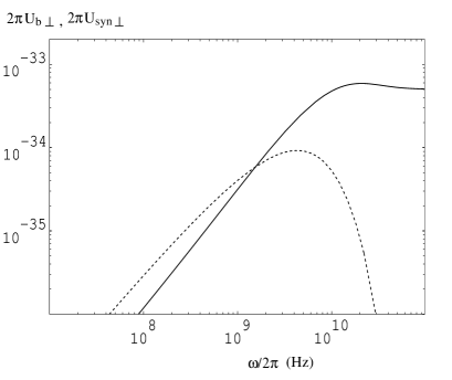
Figure 7: Energy spectrum as in figure 6 for the $\perp$-polarized components. Notice that the spectral component $2\pi U_{{\rm b}\perp}$ (solid line) tends to level out at high frequencies where the approximate form (16) applies.

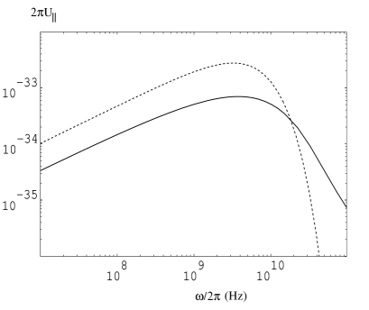
Figure 8: Energy spectrum $2\pi U_{\|}=2\pi(U_{{\rm b}\parallel}+U_{{\rm syn}\parallel})$ (in ${\rm J}\,{\rm Hz}^{-1}\,{\rm sr}^{-1}$). The dashed line corresponds to synchrotron emission $8\pi U_{{\rm syn}\parallel}$. The parameters are as in figure 6. In comparison with the normal synchrotron emission (dashed line), due to the MIB the spectrum (solid line) drops off much slower than the exponential decay at $\omega\gg\omega_{c}$.

2.4 Many-particle system

The single particle formula can be extended to a many-particle system by adding all the currents from individual particles. Let the $s$th particle be created at time $t_{s}$. A nonzero $t_{s}$ adds a phase term $\omega t_{s}$ to (5). The total current can be obtained summing up all individual currents given by (6) with all relevant quantities labelled by $s$. Then, the total energy spectrum is derived as

$$U_{\rm tot}(\omega,\hat{\mbox{\boldmath$k$}}) \approx {e^{2}\omega^{2}\over 16\pi^{3}\varepsilon_{0}c}\sum^{N}_{s,s^{\prime}=1}\biggl{[}\eta_{s}\eta_{s^{\prime}}\,(\alpha_{s}-\theta)(\alpha_{s^{\prime}}-\theta)F_{s}F^{*}_{s^{\prime}}$$ (18)

$$+{\Omega^{2}_{e}\over\gamma_{s}\gamma_{s^{\prime}}}\,\sin\alpha_{s}\sin\alpha_{s^{\prime}}\,F^{\prime}_{s}{F^{\prime}}^{*}_{s^{\prime}}\biggr{]}\,e^{i\varphi_{ss^{\prime}}},$$

where $N$ is the total number of charged particles. The coherence is determined by the phase $\varphi_{ss^{\prime}}=d_{s}-d_{s^{\prime}}$, given by

$$\varphi_{ss^{\prime}} \approx \omega(t_{s}-t_{s^{\prime}})-{\mbox{\boldmath$k$}}\cdot({\mbox{\boldmath$x$}}_{0s}-{\mbox{\boldmath$x$}}_{0s^{\prime}})$$ (19)

$$-{\omega\over\Omega_{s}}\left[1-n\beta_{s}\cos(\theta-\alpha_{s})\right](\phi-\psi_{0s})$$

$$+{\omega\over\Omega_{s^{\prime}}}\left[1-n\beta_{s^{\prime}}\cos(\theta-\alpha_{s^{\prime}})\right](\phi-\psi_{0s^{\prime}}).$$

We use the following expression for the initial position: ${\mbox{\boldmath$x$}}_{0}={\mbox{\boldmath$x$}}_{0c}-(v_{\perp}/\Omega)(\sin\psi_{0}\,{\mbox{\boldmath$e$}}_{x}-\cos\psi_{0}\,{\mbox{\boldmath$e$}}_{y})$. The usual spontaneous emission corresponds to that the phase is $|\varphi_{ss^{\prime}}|\gg 1$ for $s\neq s^{\prime}$ and that only terms of $s=s^{\prime}$ contribute to the total spectrum. Therefore in the case of spontaneous synchrotron radiation, the total spectrum can be written as $U_{\rm tot}=N\bar{U}$, where $\bar{U}$ is the single particle’s spectrum averaged over the particles’ momentum distribution. Since the initial gyrophase does not enter the final form of the energy spectrum, spontaneous synchrotron radiation is axially symmetric with respect to the magnetic field line direction, i.e. the angular pattern of emission depends only on $\theta$ not $\phi$. In the case of coherent synchrotron emission (cf. Sec. 3), such symmetry is broken since the maximum coherence depends explicitly on the initial gyrophases (cf. Eq.  19).

3 Coherent synchrotron emission

Coherent emission occurs provided that the majority of emitting particles satisfy the condition $|\varphi_{s}-\varphi_{s^{\prime}}|\ll 1$. In general, one can calculate the total spectrum numerically using (18) for a given distribution of the particle injection time, position and initial velocity. In some special cases, one may write down its analytical form. The simplest case is where all particles have the same initial velocity, which is considered here.

One may write the total spectrum into the form

$$U_{\rm tot}=N\Bigl{[}S_{\perp}(\omega)U_{\perp}+S_{\parallel}(\omega)U_{\parallel}\Bigr{]},$$ (20)

where $1\leq S_{\parallel,\perp}(\omega)\leq N$ is called the coherence factor. The value $S_{\parallel,\perp}(\omega)=N$ corresponds to completely coherent emission and $S_{\parallel,\perp}(\omega)=1$ to spontaneous emission. When the number densities of electrons and positrons are equal, $j_{\perp\theta}$ does not contribute to the coherent power as contributions from electrons and positrons cancel out. This leads to $S_{\perp}=1$. The total spectrum is

$$U_{\rm tot} = N\Bigl{[}U_{\perp}+S_{\parallel}(\omega)U_{\parallel}\Bigr{]},$$ (21)

$$U_{\parallel} \approx {e^{2}\over 16\pi\varepsilon_{0}c\sin\alpha}\left({4\omega\over\Omega_{e}\sin\alpha}\right)^{2/3}$$ (22)

$$\times\biggl{[}{{\rm Ai}^{\prime}}^{2}(\xi)+{{\rm Gi}^{\prime}}^{2}(\xi)\biggr{]},$$

where $\xi\approx(\omega/2\Omega\sin\alpha)^{2/3}[\gamma^{-2}+(\theta-\alpha)^{2}]$ and $n=1$ is assumed. In contrast to coherent Cerenkov emission, which requires a charge asymmetry (net charge) (Askar’yan 1962, 1965), coherent synchrotron emission can occur for a neutral plasma. In the case of charge symmetry, the polarization is linear, perpendicular to the plane of the magnetic field and wave vector. The coherence factor is then given by

$$S_{\parallel}(\omega)={1\over N}\sum^{N}_{s,s^{\prime}=1}\cos\left[\omega(t_{s}-t_{s^{\prime}})-{\mbox{\boldmath$k$}}\cdot({\mbox{\boldmath$x$}}_{0s}-{\mbox{\boldmath$x$}}_{0s^{\prime}})\right].$$ (23)

Eq. (23) is sum of phasors, which can be modeled as (e.g. Hartemann 2000)

$$S_{\parallel}(\omega) \approx 1-\langle\cos\Theta\rangle^{2}+N\langle\cos\Theta\rangle^{2}$$ (24)

$$+2\langle\cos\Theta\rangle\Bigl{[}N(1-\langle\cos\Theta\rangle^{2})\Bigr{]}^{1/2},$$

where $N\gg 1$, $\Theta=\omega(t_{s}-{\mbox{\boldmath$n$}}\cdot{\mbox{\boldmath$x$}}_{0s}/c)$, ${\mbox{\boldmath$n$}}={\mbox{\boldmath$k$}}c/\omega$, and the average is made over a distribution $P(\Theta)$,

$$\langle\cos\Theta\rangle\equiv\int^{2\pi}_{0}d\Theta\,P(\Theta)\cos\Theta.$$ (25)

For a uniform distribution $P(\Theta)=1$, corresponding to spontaneous emission, one has $S_{\parallel}(\omega)=1$, and for $P(\Theta)=\delta(\Theta)$, one has $S_{\parallel}(\omega)=N$, corresponding to completely coherent emission. As an example, we consider the case in which particles are injected at the same time, say at $t_{s}=0$, with a gaussian profile in the longitudinal (along $k$) spatial distribution with a width $\Delta l$. The probability can be written as

$$P(\Theta)={1\over\sqrt{\pi}\Delta\Theta}e^{-(\Theta/\Delta\Theta)^{2}},$$ (26)

where $\Delta\Theta=\omega\Delta l/c$. Then, one finds $\langle\cos\Theta\rangle=\exp(-\Delta\Theta^{2}/2)=\exp[-(\omega\Delta l/c)^{2}/2]$. A plot of $S_{\parallel}$ as a function of $\Delta l$ is shown in figure 9. Similarly, if all particles are injected at the same location with a gaussian profile with a width $\Delta t$ in time, one has $\langle\cos\Theta\rangle=\exp[-(\omega\Delta t)^{2}/2]$. This shows that to attain effective coherence, the spread in time of particle injection must be $\Delta t\sim\sqrt{2}/\omega$. The spectrum from a gaussian bunch is calculated using (20) and is shown in figure 10. The spectrum consists of two regions, separated by a critical frequency $\omega_{\rm coh}\sim(2\ln N)^{1/2}c/\Delta l$: the coherent ($S_{\parallel}>1$) emission region $\omega<\omega_{\rm coh}$, where the polarization is predominantly linear, and spontaneous ($S_{\parallel}=1$) emission region $\omega\geq\omega_{\rm coh}$, where the polarization is elliptical as both $U_{\parallel}$ and $U_{\perp}$ are present. The calculation of the coherence factor can easily be extended to other types of distribution. In particular, the $\Gamma$-probability distribution is thought to be the more relevant for air showers (Agnetta et al., 1997), which is discussed in detail in Sec. 4.

As the secondary particles from air showers have a distribution in momentum, one needs to use the full expression (18) to calculate the spectrum. When the particle’s momentum distribution is included, an analytical form for the spectrum can be derived only in some special cases. For example, when the bunch size is smaller than the relevant wavelength, one may ignore the phase term (19) and expresses the spectrum as a integration of the single particle formula over the particle’s distribution. The total intensity is about $N^{2}$ times larger than that by single particle.

Figure 9: Coherence factor vs bunch size. The solid and dashed lines correspond respectively to a gaussian bunch (26) and a bunch of $\Gamma$-form (27) with $A=5$. One assumes the total number of emitting particles $N=10^{7}$. The bunch size is in units of the wavelength $\lambda$.

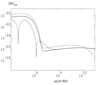
Figure 10: Spectrum $2\pi U_{\rm tot}$ (in ${\rm J}\,{\rm Hz}^{-1}\,{\rm sr}^{-1}$) from a gaussian bunch (solid line) with a longitudinal size $\Delta l=1\,\rm m$ and the $\Gamma$-pdf bunch (long-dashed line) with $A=3$. The short-dashed line corresponds to the spectrum derived by ignoring the prompt bremstrahlung. The parameters are as in figure 6. There is a critical frequency $\omega_{\rm coh}$ that separates the spectrum into the coherent region $\omega<\omega_{\rm coh}$ and spontaneous emission region $\omega\geq\omega_{\rm coh}$. For the gaussian bunch, the critical frequency is $\omega_{\rm coh}/2\pi\sim(2\ln N)^{1/2}c/2\pi\Delta l\sim 270\,\rm MHz$ and for the $\Gamma$-pdf bunch it is $\omega_{\rm coh}/2\pi\sim(c/\Delta l)N^{1/(1+A)}\approx 1\,\rm GHz$.

4 Application to air showers

The formalism developed in the previous sections can be applied to radio emission from extensive air showers (EAS). Detailed modeling requires numerical modeling of EAS, which was already considered by several authors (Suprun, Gorham & Rosner, 2003; Huege & Falcke, 2005a, b). Here we only discuss qualitatively implications of the modified synchrotron emission for radio emission from EAS and further detailed modeling will be considered elsewhere. A notable feature of the modified synchrotron emission is that the corresponding intensity derived from a semi-inifinite orbit is smaller than the conventional synchrotron emission by about a factor of 4. In principle, this feature can be tested against observations provided accurate radio spectra with well calibrated intensities become available, for example with the planned Low Frequency Array (LOFAR) (Falcke & Gorham, 2003). Other features include an angular broadening of the radiation pattern and a slower decay of the spectrum above the critical frequency ($\omega\sim\Omega_{e}\gamma^{2}$). The broadening due to prompt bremstrahlung is more pronounced for the perpendicular polarization than for the parallel polarization. Since the perpendicularly polarized component depends on the charge excess, such broadening is important when there is significant charge asymmetry. The spectral hardening occurs near the synchrotron cut-off frequency, which is much higher than the transition frequency $\omega_{\rm coh}$. So, this spectral feature may not be observable for air showers.

In the following we derive the coherence factor using the procedure in Sec. 3. As an example, one assumes that an air shower occurs at a few km height and that all emitting particles are located in the shower maximum. As the zeroth order approximation, the near field effect can be ignored and the energy spectrum (Eq. 18) derived in Sec. 2 is applicable. The near field effect may need to be included if the maximum of an air shower develops very near the ground level. There are extensive discussions of air showers in the literature (Gaisser, 1990) and in principle, one can obtain a distribution of particle’s injection time ($t_{s}$), initial momentum ($\gamma{\mbox{\boldmath$v$}}_{0s}$) and position (${\mbox{\boldmath$x$}}_{0s}$). Assuming the primary cosmic ray energy to be $E_{p}$, the number of secondary electrons and positrons can be estimated as $N\sim E_{p}/\gamma m_{e}c^{2}\sim 10^{7}$ for $E_{p}\sim 10^{15}\,\rm eV$ and $\gamma=80$. In the practical situation these particles are injected over an extended range rather than at a single fixed height. For EAS, the distribution in $t_{s}$ for secondary electrons/positrons can be inferred from measurements of arrival times of charged particles (muons plus electrons/positrons). One should note that these measured times are not actual arrival times of electrons and positrons since muons arrive earlier than electrons/positrons. The arrival times can be modeled by a $\Gamma$-probability distribution function ($\Gamma$-pdf) (Agnetta et al., 1997; Antoni, et al., 2001). Thus, the probability can be written as (Huege & Falcke, 2003):

$$P(\Theta)={1\over\Delta\Theta\Gamma(1+A)}\,\left({\Theta\over\Delta\Theta}\right)^{A}\,e^{-\Theta/\Delta\Theta},$$ (27)

for $\Theta>0$ and $P(\Theta)=0$ for $\Theta\leq 0$, where $\Gamma(x)$ is the Gamma function and the power index $A$ can be estimated from the distribution of electrons arrival times. The standard deviation is $\sigma_{\Gamma}=(1+A)^{1/2}\Delta\Theta$. From (27), one obtains

$$\langle\cos\Theta\rangle=\left(1+\Delta\Theta^{2}\right)^{-(1+A)/2}\cos\biggl{[}(1+A)\arctan\Delta\Theta\biggr{]},$$ (28)

$$\langle\Theta\rangle=(1+A)\Delta\Theta.$$ (29)

The corresponding critical frequency is given by $\omega_{\rm coh}\sim(c/\Delta l)N^{1/(1+A)}$. This frequency defines a transition from coherent to incoherent emission. For $\Delta l=1\,\rm m$, $N=10^{7}$ and $A=5$, one has $\omega_{\rm coh}/2\pi\sim 1.2\,\rm GHz$. The coherence factor can be obtained by substituting (28) for (24). Here we write down the two limiting cases:

$$S_{\parallel}\approx\left\{\begin{array}[]{ll}N(1+\Delta\Theta^{2})^{-1-A}&\\ \quad\quad\times\cos^{2}\biggl{[}(1+A)\arctan\Delta\Theta\biggr{]},&\omega<\omega_{\rm coh},\\ 1,&\omega\gg\omega_{\rm coh}.\end{array}\right.$$ (30)

The dashed line in figure 9 shows $S_{\parallel}$ as a function of the bunch size $\Delta l$, featuring a higher transition frequency $\omega_{\rm coh}$ than the gaussian bunch. The low-frequency approximation in (30) corresponds to the nonsquared form given by Huege & Falcke (2003) except that the cosine factor is retained here.

The coherent emission can be elliptically polarized if there is a charge excess as it is the case for air showers. Assuming the excess number of electrons is $N_{c}$, one has

$${S_{\perp}\over S_{\parallel}}\sim{N_{c}\over N}.$$ (31)

The right-hand side is sensitive to the cut-off energy of the excess electron energy. For a cut-off near the MeV energy, the excess of electrons can reach $N_{c}/N\sim 10-15\%$. (Note that cascades in a dense medium such as rocks can give rise to about $N_{c}/N\sim 20\%$ excess negative charge.) As a result, the coherent emission can be elliptically polarized with an ellipticity $\sim(S_{\perp}/S_{\parallel})^{1/2}\delta_{c}=(N_{c}/N)^{2}\delta_{c}\sim 0.3\delta_{c}$, where $\delta_{c}$ is the typical ellipticity of single particle’s radiation.

5 Conclusions

Synchrotron emission by a particle moving along a semi-infinite trajectory is considered. Since effective coherent synchrotron emission by secondary particles in an air shower occurs in the core of the shower where most emitting particles are created, the initial point of the particle’s trajectory need be included explicitly. It is shown that radiation from a particle moving along a semi-infinite track can be separated into the usual synchrotron emission and the bremsstrahlung-like emission (MIB). The latter is due to emission as the result of onset of the particle’s curved trajectory. The spectral intensity of the modified synchrotron emission (usual synchrotron plus MIB) is lower than that for normal synchrotron emission, roughly by a factor of 4. It is interesting to note that such reduction is consistent with the recent result from numerical simulation by Huege & Falcke (2005b). The radiation pattern has a broader angular distribution than the usual synchrotron emission. This feature is especially pronounced for the perpendicularly polarized component. The spectrum has a much slower decay above the critical frequency $\omega\sim\gamma^{2}\Omega_{e}$, while the usual synchrotron spectrum has an exponential cutoff above the critical frequency. In the application to radio emission from air showers, the reduced intensity can be verified in principle provided accurate observations of the radio spectrum are available. Although there exist early observations of air shower radio emission, there are some uncertainties in determining the calibration factor (Allan, 1971; Atrashkevich et al, 1978). The current LOFAR Prototype Station (LOPES) and the future LOFAR may provide a better opportunity to test the predicted spectrum. Since the transition frequency (to spontaneous emission) is much lower than the cut-off frequency, change near the cut-off frequency may not be observable. The broadening of the radiation pattern occurs mainly for the perpendicularly polarized component, which may be observable provided that there is significant charge asymmetry in the emitting plasma.

A major advantage of the formalism presented here is that the initial conditions including the time of particle creation, initial velocity and gyrophase all appear in the phase (19) and these quantities can be modeled statistically. Although the single-particle formalism was used by White & Melrose (1982) to treat coherent gyromagnetic emission, in their calculation, the finite track effect was not considered. It is shown here that the distribution of the particle injection time is important in determining the coherence. The semi-infinite track approximation adopted here is valid provided that the emitting particles are highly relativistic with $\gamma\gg 1$. In the relativistic limit, the synchrotron pulse duration ($1/\Omega_{e}\gamma^{2}\sim 10^{-8}\,\rm s$) is much shorter than the typical flight time $T\sim 10^{-6}\,\rm s$ for a particle’s free path 500 m, and therefore the orbit can be approximately regarded as semi-infinite. If electrons and positrons from an air shower have an energy cutoff extending to MeV energies with $\gamma\sim 1$, the synchrotron approximation is no longer valid and one has cyclotron emission instead. In this case, a finite orbit needs to be considered. One may extend the calculation in Sec. 3 and 4 to include the particle distribution in momentum and this requires a numerical approach, which is not considered here.

References

- Abramowitz & Stegun (1991) Abramowitz, M., Stegun, I., 1991, Handbook of Mathematical Functions (New York: Dover Publications).
- Agnetta et al. (1997) Agnetta, G. et al. 1997, Astroparticle Phys. 6, 301.
- Allan (1971) Allan, H. R., 1971, in Progress in Elementary Particles and Cosmic Ray Physics, Vol. 10, p. 171.
- Aloisio & Blasi (2002) Aloisio, R. & Blasi, P. 2002, Astroparticle Phys. 18, 183.
- Alvarez-Muñiz, Vázquez, & Zas (2000) Alvarez-Muñiz, J., Vázquez, R. A., & Zas, E., 2000, Phys. Rev. D62, 063001.
- Antoni, et al. (2001) Antoni, T. et al. 2001, Astroparticle Phys. 14, 245.
- Arskar’yan (1962) Askar’yan, G. A. 1962, Sov. Phys. JETP, 14, 441.
- Arskar’yan (1965) Askar’yan, G. A. 1965, Sov. Phys. JETP, 21, 658.
- Atrashkevich et al (1978) Atrashkevich, V. B. et al., 1978, Sov. J. Nucl. Phys. 28, 366.
- Colgate (1967) Colgate, S. A., 1967, J. Geophys. Res. 72, 4869.
- Dagkesamanskii & Zheleznykh (1989) Dagkesamanskii, R. D. & Zheleznykh, M., 1989, JETP Lett. 50, 259.
- Falcke et al. (2005) Falcke, H. et al. 2005, Nature, 435, 313.
- Falcke & Gorham (2003) Falcke, H. & Gorham, P., Astrop. Phys. 19, 477.
- Falcke, Gorham, & Protheroe (2004) Falcke, H., Gorham, P., & Protheroe, R. J., 2004, New Astron Rev. 48, 1487.
- Gaisser (1990) Gaisser, T. K., 1990, Cosmic Rays and Particle Physics (Cambridge: University Press).
- Gorham, et al. (2004) Gorham, P. W., et al., 2004, Phys. Rev. Lett. 93, 041101.
- Grichine (2003) Grichine, V. M., 2003, Radiation Phy. & Chem. 67, 93.
- Hankins, Ekers, & O’Sullivan (1996) Hankins, T., Ekers, R., & O’Sullivan, J. D., 1996, MNRAS, 283, 1027.
- Hartemann (2000) Hartemann, F., 2000, Phys. Rev. E61, 972.
- Huege & Falcke (2005a) Huege, T. & Falcke, H., 2005, Astroparticle Phys. 24, 116.
- Huege & Falcke (2005b) Huege, T. & Falcke, H., 2005, A&A, 430, 779.
- Huege & Falcke (2003) Huege, T. & Falcke, H., 2003, A&A, 412, 19.
- Jackson (1998) Jackson, J. D., 1998, Classical Electrodynamics (New York: Wiley).
- Kahn & Lerche (1966) Kahn, F. D. & Lerche, I., 1966, Proc. R. Soc. London, A289, 206.
- Landau & Lifshitz (1971) Landau, L. D. & Lifshitz, E. M., 1971, The Classical Theory of Fields (Oxford: Pergamon Press).
- Melrose (1986) Melrose, D. B., 1986, Instabilities in Space and Laboratory Plasmas, Cambridge University Press.
- Melrose & McPhedron (1991) Melrose, D. B., McPhedron, R. C., 1991, Electromagnetic processes in dispersive media, Cambridge U. press.
- Suprun, Gorham & Rosner (2003) Suprun, D. A., Gorham, P. W., & Rosner, J. L., 2003, Astroparticle Phys. 20, 157.
- Tamm (1939) Tamm, I. E., 1939, J. Phys. (Moscow) 1, 439.
- White & Melrose (1982) White, S. M. & Melrose, D. B., 1982, PASA 4, 362.
- Zas, Halzen & Stanev (1992) Zas, E., Halzen, F., & Stanev, T., 1992, Phys. Rev. D45, 362.