Constraining Torus Models for AGNs Using X-ray Observations

Abstract

Context. In Unification Models, Active Galactic Nuclei (AGN) are believed to be surrounded by an axisymmetric structure of dust and gas, which greatly influences their observed properties according to the direction from which they are observed.

Aims. The main aim of this work is to constrain the properties of this obscuring material using X-Ray observations.

Methods. The distribution of column densities observed by $Chandra$ in the Chandra Deep Field South is used to determine geometrical constraints for already proposed torus models.

Results. It is found that the best torus model is given by a classical ‘donut shape’ with an exponential angular dependency of the density profile. The opening angle is strongly constrained by the observed column densities. Other proposed torus models are clearly rejected by the X-Ray observations.

Conclusions.

1 Introduction

A unified scheme to explain a variety of Active Galactic Nuclei (AGNs) has been proposed by Antonucci (antonucci (1993)) to explain the differences observed in Seyfert galaxies, a class of local active galaxies. According to this Unification Model, the active nucleus is surrounded by a toroidal structure composed of gas and dust, which determines dramatic spectral differences depending on our line of sight towards the central source. In the X-Ray domain, if an AGN has a neutral Hydrogen column density ($N_{H}$) in the line of sight smaller (when viewed face-on) or larger (when viewed edge-on) than $10^{22}$ cm^-2, then the object is classified as Type I or Type II, respectively.

The dusty toroidal structure that surrounds the central source absorbs the optical, ultraviolet and soft X-Ray emission from the active nucleus. However, hard X-Ray photons ($>2$ keV) can partially escape from this cold material. Therefore, from X-Ray observations it is possible to measure the column density in the line of sight, and put tight constraints on the properties of the obscuring medium.

It is commonly believed that this X-Ray emission is produced in a ’corona’ near the super-massive black hole, where low energy photons from the accretion disk are reprocessed by energetic electrons (either mildly relativistic thermal electrons or highly relativistic non-thermal electrons) via Inverse Compton Scattering. The main result of this process is an observed spectral energy distribution described by a power law, with a typical slope $\Gamma\approx 1.8$ (Turner et al. turner (1997), Tozzi et al. tozzi (2006)), and an exponential cutoff energy at $\approx 300$ keV (Matt et al. matt (1999)). The radiation can also be reflected and/or scattered depending on the circumnuclear material distribution causing the overall spectral shape to become flatter, $\Gamma\approx 1.7$, with an apparent smaller energy cutoff (see Svensson svensson (1996)).

As hard X-Ray energy photons can penetrate the surrounding material, and eventually escape from the AGN host, they can be detected with the present generation of X-Ray telescopes. But if the Hydrogen column density along the line of sight becomes larger than the inverse of the photoelectric Cross Section $\sigma_{10{\rm keV}}^{-1}\approx 10^{24}$ cm^-2 (see Matt matt02 (2002)), then the medium becomes Compton Thick ($\tau=N_{H}\sigma\approx 1$). In this case, the only observable emission component is coming from photons scattered and/or reflected by the circumnuclear media (Wilman & Fabian wil_fab (1999)).

Since Compton Thin AGNs (those with $N_{H}<10^{24}$ cm^-2) are ubiquitous emitters in the $2-10$ keV hard X-Ray band, deep X-Ray surveys have proven to be the best way to estimate the number density and evolution of active galaxies in the Universe (Mushotzky Mushotzky (2004)). Unfortunately, these X-Ray surveys are always flux limited (nowadays $F^{\mbox{\scriptsize{limit}}}_{\mbox{\scriptsize{2-10keV}}}\approx 10^{-16}$ erg sec^-1 cm^-2), and therefore biased against faint sources. In fact, the population of high redshift, low luminosity, and highly obscured AGNs is still not well determined. This problem translates into a poorly determined faint end of the luminosity function, implying uncertainties in the contribution of obscured AGNs to the Cosmic X-Ray Background (CXRB), which is known to require of a sizable population of obscured sources in order to explain its hard spectral energy distribution.

The aim of the present work is to constrain different torus geometries that can reproduce the observed distribution of Hydrogen column densities ($N_{H}$) in AGNs observed by $Chandra$ in the Chandra Deep Field South (CDF-S).

Section 2 describes the intrinsic $N_{H}$ distribution found by Tozzi et al. (tozzi (2006)) which was used in our analysis. In Section 3 we explain the theoretical modelling, while in Section 4 we present our models and results. In Section 5 our results are discussed and we present the conclusions in Section 6. Throughout this work we use: $\Omega_{m}=0.3$, $\Omega_{\Lambda}=0.7$ and $H_{0}=70$ km sec^-1 Mpc^-1 (Spergel et al. spergel (2003)).

2 Deep X-Ray Observations

2.1 AGNs in the $Chandra$ Deep Field-South

In the past few years, several deep $Chandra$ images of the extragalactic sky have been obtained, with the $2\ Ms$ $Chandra$ Deep Field-North (CDF-N; Alexander et al. Alex (2003)) and $1\ Ms$ $Chandra$ Deep Field-South (CDF-S; Giacconi et al. Giac (2002)) being the two deepest ($F^{\text{limit}}_{2-10\ keV}\approx 1.4\cdot 10^{-16}$ erg s cm² for CDF-N and a factor 2 shallower for the CDF-S). Optical identifications have been obtained for most X-Ray sources in these fields. Barger et al. (Barger03 (2003)) presented multicolour imaging data for all 503 X-Ray point sources in the CDF-N and spectroscopic redshifts for $\sim 56\%$ of the sample. Zheng et al (zheng (2004)) presented accurate photometric redshifts for 342 sources in the CDF-S using the large multicolour data set available for this field. This corresponds to $\sim 99\%$ of the sample and includes 173 sources with reliable spectroscopic redshifts from Szokoly et. al (Szok (2004)).

Given the photo-z completeness of $\sim 99\%$ for the the X-Ray sources in the CDF-S, this field becomes the perfect choice for our study of the torus properties. Redshifts are necessary in order to compute the observed $N_{H}$ (see below) as well as the source X-Ray luminosity.

Following the sample definition for the CDF-S found in Tozzi et al. (tozzi (2006)), out of the 347 X-Ray detected sources (346 sources presented by Giacconi et al. (Giac (2002)) and 1 extra source presented by Szokoly et al. (Szok (2004))), 7 sources are stars and 4 have no redshift information. Further 15 sources have X-Ray luminosities $<10^{41}$ erg s^-1 cm^-2, a luminosity range where emission from star forming galaxies becomes significant, and are therefore discarded. Finally, 14 Compton Thick AGN were also eliminated, as discussed in Section 4. The final sample contains 307 X-Ray point sources at $z>0$ that will be used for our study.

2.2 Hydrogen Column Densities

The distribution of $N_{H}$ values for the sources in the CDF-S were derived by Tozzi et. al (tozzi (2006)). They performed direct X-Ray spectral fitting to the observed Chandra data using the redshift information published by Zheng et. al (zheng (2004)). Using a subsample with the 82 brightest sources, Tozzi et. al (tozzi (2006)) determined a weighted mean spectral index of $\Gamma\sim 1.75$ which resulted independent of the values of the derived $N_{H}$. By fixing $\Gamma=1.8$ the redshifted $N_{H}$ was derived for the rest of the sample. The distribution was then corrected for incompleteness in the luminosity and redshift parameter space using the survey effective area and the luminosity function of Ueda et al. (Ueda (2003)). Ueda’s luminosity function was determined using 247 AGN detected in the $2-10$ keV X-Ray band from a compilation of $ASCA$, $HEAO-1$ and $Chandra$ observations. The luminosity function shows a luminosity dependent density evolution, in which the low luminosity AGN population peaks at a lower redshift than the high luminosity sources. This is consistent with optical quasar observations in which this population peaks at redshift $\sim 2$ (Boyle et al. boyle (2000)).

The final corrected $N_{H}$ distribution, seen in Figure 16 of Tozzi et. al (tozzi (2006)), will be used in the following sections to constrain the torus parameters.

3 Model General Properties

We first assume that the X-Ray emission in AGNs comes from the nearest region to the super-massive black hole. This region has a typical spatial scale of $R_{C}\approx 10-100\ R_{S}$ (where $R_{S}=GM_{BH}/c^{2}$ is the Schwarzschild Radius), implying physical sizes of $R_{C}\approx 10^{-5}-10^{-3}$ pc for a typical super-massive black hole with $M_{BH}\approx 10^{7}-10^{8}\ M_{\odot}$. Recent observations of NGC 1068 using mid-infrared interferometry, suggest a torus about $3.4$ pc diameter (Jaffe et al. jaffe (2004)), while near-IR reverberation mapping of nearby Seyfert galaxies estimates an inner limit at $\sim 10^{-2}-10^{-1}$ pc (Suganuma et al. Suganuma06 (2006)). Therefore, for practical purposes we can approximate the X-Ray source as a point-like emitting region, implying an easy treatment for the X-Ray radiation that will provide the total column density along the line of sight.

3.1 Torus Properties

We consider four different torus models (presented in Section 4) to obtain synthetic distributions of column densities which are then compared with the observed distribution from Tozzi et. al (tozzi (2006)).

We model the obscuring region as a simple axisymmetrical matter distribution surrounding the accretion disk. Given the symmetry of the problem, random lines of sight with polar angles between 0 and $\pi/2$ (weighted by the angle differential area), are used to calculate the optical depth for each random direction, where the the polar angle $\phi$ is defined as the angle subtended between the line of sight and the torus equatorial plane.

We assume a solar abundance for the torus, a photoelectric cross section for absorption given by Morrison & McCammon (MoMc (1983)), a standard Galactic Gas-to-Dust ratio $N_{H}/E(B-V)=5.8\cdot 10^{21}$ cm^-2 given by Bohlin et al. (Bohlin (1978)) and a solar neighbourhood value $R_{V}=3.1$ (Schultz & Weimer sch_wei (1975)). These assumptions relate the Hydrogen column density $N_{H}$ with the optical extinction $A_{V}$, and the optical depth $\tau_{V}$ ($A_{V}=1.09\tau_{V}$),

$$\begin{split}N_{H}(\phi)&=\sigma^{-1}\tau=\int\rho(r,\phi)dr\\ &=5.8\cdot 10^{21}\ E(B-V)\ {\rm cm}^{-2}=1.9\cdot 10^{21}A_{V}\ {\rm cm}^{-2}\\ &=2.0\cdot 10^{21}\tau_{V}\ {\rm cm}^{-2}=2.0\cdot 10^{21}\ \tau_{Vi}\ N_{T}\ {\rm cm}^{-2}\end{split}$$ (1)

where, if the medium is continuous, $\rho(r,\phi)$ is the matter density distribution and $\sigma$ the effective absorption cross section. Otherwise, if the medium is clumpy, $\tau_{Vi}$ represents the optical depth for one cloud and $N_{T}$ the average number of clouds along the line of sight. It is easy to show that if the density distribution $\rho$ has no angular dependency (i.e., $\rho=\rho(r)$), then the radial dependency will be hidden by the assumed maximum column density $N_{Hmax}$ along the line of sight (see Section 4).

Other model parameters, such as the inner radius, external radius, density in the equatorial plane, and/or cloud optical depth, are also constrained by $N_{Hmax}$. In this work we fix the maximum value for the column density at $N_{Hmax}=10^{25}$ cm^-2, according to X-Ray observations of Type II AGNs in the $0.1-100$ keV band using the BeppoSAX X-Ray satellite (Maiolino et al. Maiolino (1998)).

Due to the degeneracy of the model parameters, we use the minimum number possible of free parameters to describe the torus distribution. The chosen parameterisations do not give physical sizes of the distributions explicitly, but instead reduced parameters such as $R_{int}/R_{out}$ (where $R_{out}$ is the external radius and $R_{int}$ is the inner radius for the torus) are used. $R_{int}$ can be estimated by the ‘evaporation radius’ for graphites (at $T\approx 1500\ K$) defined by assuming thermal equilibrium between the ultraviolet incident radiation and the rate for reemission from the dust. Assuming $a_{\mbox{\scriptsize{gr}}}=0.05\ \mu$m as a typical grain size, and following Barvainis (bar (1987)),

$$R_{int}\approx 0.4L_{UV,45}^{1/2}\ {\mbox{\scriptsize{\small{pc}}}},$$ (2)

where $L_{UV,45}$ is the ultraviolet (UV) luminosity per unit of $10^{45}$ erg sec^-1. Assuming this value as a lower limit for the distance, we can estimate the external radius $R_{out}$, and other model parameters using our torus model results (see estimations in Table 1).

4 Modelling the Torus

The large degeneracy of model parameters and the uncertainties given by the lack of faint sources in the $N_{H}$ distribution determined by Tozzi et al. (tozzi (2006)), require us to keep the number of free parameters within our torus models to a minimum. As such, we do not allow the parameters to change with luminosity or redshift.

Barger et al. (Barger05 (2005)) presented a complete sample of local X-Ray selected AGN ($z<1.2$), in which a luminosity dependence for the fraction of Type II over Type I AGNs is seen, as Ueda et al. (Ueda (2003)) proposed earlier. This implies a possible dependency of the covering factor of the dusty torus on luminosity, and therefore a change in the geometrical torus distribution. Hence, our results can be understood as an average geometrical distribution for the entire AGN population, given by a simple axially symmetric geometry, with no dependency on luminosity or redshift. A discussion on the luminosity dependency can be found in Section 5.

To determine the torus parameters which best fit the observed column densities, we use the $\chi^{2}$ test assuming poissonian error bars for the observed data. Our own experience determining the intrinsic $N_{H}$ distribution based on Hardness Ratio measurements suggests that this method introduces large uncertainties in the inferred $N_{H}$ values, which dominate over the poissonian errors from a population of sources. On the other hand, the spectral treatment introduced by Tozzi et al. (tozzi (2006)) gives more reliable values for the intrinsic properties of the obscuring region present in AGNs.

Tozzi et al. (tozzi (2006)) found 14 sources showing a reflection-dominated spectrum. These Compton Thick sources were not used in our analysis because of the large uncertainties in the number counts of this population. In fact, we have not used the last bin in the intrinsic column density distribution shown in Figure 16 of Tozzi et al. tozzi (2006), which includes objects with $N_{H}>10^{24}$ cm^-2 and corresponds to a lower limit only.

The models presented in the remaining of this section were motivated by previous work which were carried out to explain a variety of observational properties of AGNs (Treister et al. Treister (2004); Pier & Krolik pi_kr92 (1992), pi_kr93 (1993); Granato & Danese gr_da (1994); Elitzur et al. Elitzur (2003)). A summary of the results from the modelling is presented in Table 1.

4.1 Model 1

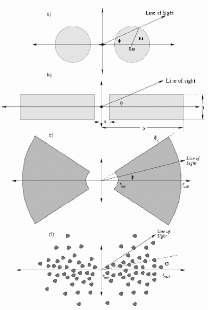
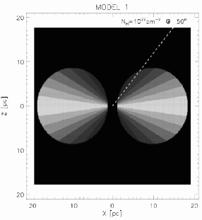
Following the torus distribution proposed by Treister et al. (Treister (2004)), we modelled the geometry given by Figure 1a to find different optical depths as a function of the line of sight, $\phi$. In this case the matter density is not distributed as in an homogeneous medium, but has the following dependence with $\phi$ and $r$:

$$\rho(r,\phi)=\rho_{\mbox{\scriptsize{eq}}}\left(\frac{r_{\mbox{\scriptsize{int}}}}{r}\right)^{\beta}\ e^{-\gamma\left|\sin(\phi)\right|}$$ (3)

where $\rho_{\mbox{\scriptsize{eq}}}$ is the inner density (at $r_{\mbox{\scriptsize{int}}}=R_{m}-R_{t}$) in the equatorial plane (constrained by $N_{Hmax}$, see Equation 5). In this model, the free parameters are $R_{m}/R_{t}$ (see Figure 1a), $\gamma$, and $\beta$. The analytical equations which describe the column density as a function of $\phi$ are given by:

$$\begin{array}[]{rl}&{\mbox{\scriptsize{\small{If}}}}\quad 0\leq\phi<\sin^{-1}\left(R_{t}/R_{m}\right)\quad{\mbox{\scriptsize{\small{and}}}}\quad\beta\neq 1\quad{\mbox{\scriptsize{\small{then,}}}}\\ &N_{H}=N_{Hmax}\ e^{-\gamma\left|\sin(\phi)\right|}\ \times\\ &\quad\quad\frac{\left[\left(\cos(\phi)+\sqrt{(R_{t}/R_{m})^{2}-\sin(\phi)^{2}}\right)^{1-\beta}-\left(\cos(\phi)-\sqrt{(R_{t}/R_{m})^{2}-\sin(\phi)^{2}}\right)^{1-\beta}\right]}{(1+R_{t}/R_{m})^{1-\beta}-(1-R_{t}/R_{m})^{1-\beta}}\\ &{\mbox{\scriptsize{\small{If}}}}\quad 0\leq\phi<\sin^{-1}\left(R_{t}/R_{m}\right)\quad{\mbox{\scriptsize{\small{and}}}}\quad\beta=1\quad{\mbox{\scriptsize{\small{then,}}}}\\ &N_{H}=N_{Hmax}\ e^{-\gamma\left|\sin(\phi)\right|}\ \times\\ &\quad\quad\frac{\ln\left(\left(\cos(\phi)+\sqrt{(R_{t}/R_{m})^{2}-\sin(\phi)^{2}}\right)/\left(\cos(\phi)-\sqrt{(R_{t}/R_{m})^{2}-\sin(\phi)^{2}}\right)\right)}{\ln\left((1+R_{t}/R_{m})/(1-R_{t}/R_{m})\right)}\\ &{\mbox{\scriptsize{\small{If}}}}\quad\sin^{-1}\left(R_{t}/R_{m}\right)\leq\phi\leq\pi/2\quad{\mbox{\scriptsize{\small{then,}}}}\quad N_{H}=N_{Hmin}\end{array}$$ (4)

The maximum and minimum column density along the line of sight is through the equatorial plane and at the poles, respectively.

$$\begin{split}{\mbox{\scriptsize{\small{If}}}}\quad&\beta\neq 1\quad{\mbox{\scriptsize{\small{then,}}}}\quad\\ &N_{Hmax}=\rho_{\mbox{\scriptsize{eq}}}\ r_{\mbox{\scriptsize{int}}}^{\beta}\frac{R_{m}^{1-\beta}}{1-\beta}\left[\left(1+\frac{R_{t}}{R_{m}}\right)^{1-\beta}-\left(1-\frac{R_{t}}{R_{m}}\right)^{1-\beta}\right]\\ {\mbox{\scriptsize{\small{If}}}}\quad&\beta=1\quad{\mbox{\scriptsize{\small{then,}}}}\quad N_{Hmax}=\rho_{\mbox{\scriptsize{eq}}}\ r_{\mbox{\scriptsize{int}}}\ln\left(\frac{1+R_{t}/R_{m}}{1-R_{t}/R_{m}}\right)\\ \end{split}$$ (5)

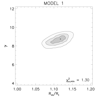
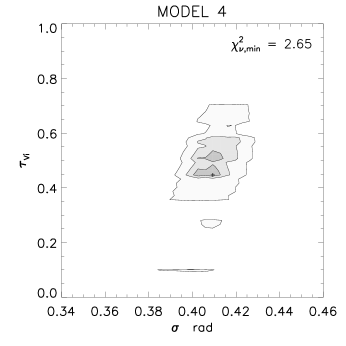
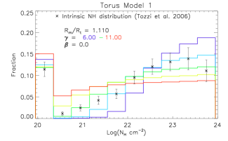
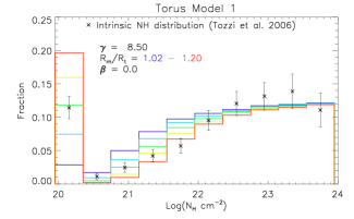
This model gives a good fit to the data, with $\chi^{2}_{\nu,min}=1.30$. Results adopting $\beta=0.0$ are presented in Figure 2 and show a well constrained region of the $R_{m}/R_{t}-\gamma$ parameter space. The best fit values are spread between $1.07\lesssim R_{m}/R_{t}\lesssim 1.15$ and $7.0\lesssim\gamma\lesssim 9.0$ at 3 $\sigma$ confidence levels. The same results are obtained when a value $\beta=2.0$ is adopted. Adopting $\beta=1.0$ and $3.0$ results in a small decrease in the value of $\gamma$, but does not introduce further changes. Note however, that $\beta$ modifies the value of $N_{Hmax}$ through Equation 5.

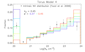
From the family of parameters found, we show in figure 3 some examples of synthetic $N_{H}$ distributions and compared them with the one determined by Tozzi et al. (tozzi (2006)). It is seen that the parameter $R_{m}/R_{t}$ mostly affects the distribution of Type I sources (i.e., for $N_{H}<10^{22}$ cm^-2), while $\gamma$ changes the Type II/I fraction.

A sketch of the torus geometrical distribution, choosing the best fit parameters, is given in Figure 4, where the ‘donut’ structure of the model is clearly seen. Under these assumed parameters, this model predicts an intrinsic fraction of sources with column densities $>10^{24}$ cm^-2 of $\sim 27\%$.

Model	$\chi^{2}_{\nu,min}$	Parameter 1	Parameter 2	Parameter 3	$R_{\mbox{\scriptsize{out}}}[pc]$	$\rho_{\mbox{\scriptsize{eq}}}[cm^{-3}]$
1	$1.30$	$1.07\lesssim R_{m}/R_{t}\lesssim 1.15$	$7.0\lesssim\gamma\lesssim 9.0$	$0.0\lesssim\beta\lesssim 3.0\phantom{.}^{\ddagger}$	$5.7-12$	$2.8-6.0\cdot 10^{5}\phantom{.}{}^{\dagger}$
2	$8.13$	$2.4\lesssim h/a\lesssim 3.3$	$250\lesssim b/a\lesssim 600$	X	$100-240$	$1.3-3.2\cdot 10^{4}$
3	$5.65$	$1.0\lesssim\phi_{c}\ rad\lesssim 1.2$	$8.0\lesssim\gamma\lesssim 10.0$	$free$	$1.0\phantom{.}^{\ast}$	$5.4\cdot 10^{6}\phantom{.}{}^{\dagger}$
4	$2.65$	$0.38\lesssim\sigma\ rad\lesssim 0.44$	$\tau_{Vi}\lesssim 0.8$	X	$free$	-

Notes .-
$\phantom{.}{}^{\ast}$ indicate a fixed parameter.
$\phantom{.}{}^{\dagger}$ these parameters can be modified taking into account radial dependencies for the model, i.e. $\beta\neq 0$.
$\phantom{.}{}^{\ddagger}$ obtained assuming $\gamma=9.0$.

Table 1: Summary of the estimated parameters for the models described in Section 4. Ranges are obtained from 3 $\sigma$ confidence limits (see contour plots in the Figure 2). The last two columns are deduced considering a UV luminosity of $10^{45}$ erg sec^-1 and Equation 2. No radial dependency for the density distribution ($\beta=0.0$) is assumed in the models. In Model 3 we use a fixed parameter $R_{\mbox{\scriptsize{out}}}=1$ pc to estimate a density at the equatorial plane, although this is a free parameter. Model 4 is not shown in the last columns due to the different cloud treatment explained in Subsection 4.4.

4.2 Model 2

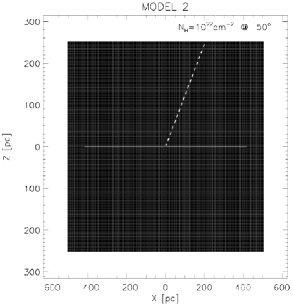
This model is proposed following previous studies by Pier & Krolik (pi_kr92 (1992), pi_kr93 (1993)) based on the IR reemission coming from the torus. We use their geometrical distribution (Figure 1b) to find the dependency of the column density with the line of sight.

This model assumes a homogeneous density with $h/a$ and $b/a$ as free parameters, where $h$, $b$, and $a$ are as shown in Figure 1b. The dependency of the column density with the line of sight ($0\leq\phi\leq\pi/2$) is given by:

$$\begin{array}[]{rl}{\mbox{\scriptsize{\small{If}}}}&\quad 0\leq\phi<\tan^{-1}\left(\frac{h}{2b}\right)\quad{\mbox{\scriptsize{\small{then,}}}}\quad N_{H}=N_{Hmax}\frac{\cos\left(\tan^{-1}\left(h/2b\right)\right)}{\cos(\phi)}\\ {\mbox{\scriptsize{\small{If}}}}&\quad\tan^{-1}\left(\frac{h}{2b}\right)\leq\phi<\tan^{-1}\left(\frac{h}{2a}\right)\quad{\mbox{\scriptsize{\small{then,}}}}\\ &N_{H}=N_{Hmax}\frac{\cos\left(\tan^{-1}\left(h/2b\right)\right)}{b/a-1}\left(\frac{h}{2a}\sin(\phi)^{-1}-\cos(\phi)^{-1}\right)\\ {\mbox{\scriptsize{\small{If}}}}&\quad\tan^{-1}\left(\frac{h}{2a}\right)\leq\phi\leq\pi/2\quad{\mbox{\scriptsize{\small{then,}}}}\quad N_{H}=N_{Hmin}\end{array}$$ (6)

where the maximum column density is:

$$N_{Hmax}=\rho_{\mbox{\scriptsize{eq}}}\ \frac{b-a}{\cos\left(\tan^{-1}\left(\frac{h}{2b}\right)\right)}$$ (7)

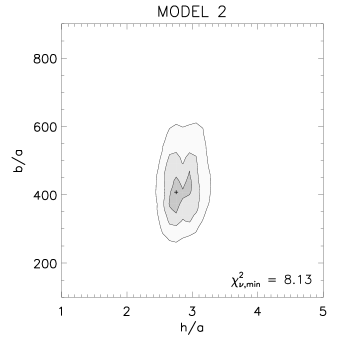
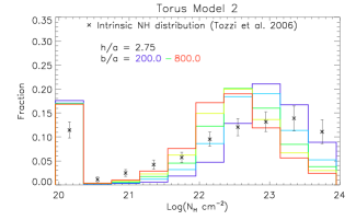
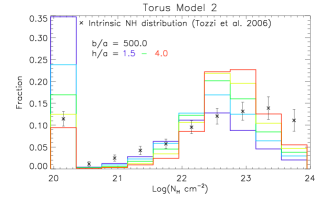
Comparing the synthetic distributions of column densities with the observed one, we found the results shown in Figure 2. The parameters are not well constrained and imply $2.4\lesssim h/a\lesssim 3.3$ and $250\lesssim b/a\lesssim 600$ at 3 $\sigma$ confidence levels. The model also shows an extreme radial-to-vertical thickness ratio ($b/h\approx 75-250$).

Synthetic $N_{H}$ histograms are shown in Figure 3. It is seen that the parameter $b/a$ systematically overestimates the number of sources at around $N_{H}=10^{22.5}\ cm^{-2}$, while $h/a$ modifies the first bin of unobscured sources.

Clearly, this model is limited by its constant density distribution. This translates into a large $b/a$, needed to reproduce the wide range of observed column densities (since $N_{H}\propto\Delta s$), and a very sensitive distribution in the innermost region of the torus (see Figure 4). Also, the model does not predict a large fraction of highly obscured sources, implying that it cannot explain the CXRB or the number of Compton Thick sources observed in the CDF-S ($\sim 10\%$; Tozzi et al. tozzi (2006)). The typical intrinsic fraction of Compton Thick sources predicted by the model is only $\sim 3\%$ which are produced by a narrow angular section near the equatorial plane able to account for large column densities (see Figure 4).

When we compare our analysis with the results by Pier & Krolik (pi_kr92 (1992)), we find further disagreements. Typical dimensions deduced by them, as restricted by IR torus reemission, are of parsec-scale, meanwhile we obtain a torus with typical scales of $\sim 200$ pc assuming $L_{UV}=10^{45}$ erg sec^-1.

We conclude that this torus model can be rejected due to the numerous caveats already discussed, such as typically large outer radius, which is not seen in local AGNs (Jaffe et al. jaffe (2004); Prieto et al prieto (2004)), the sensibility of the geometrical distribution in the inner regions, and the small number of predicted Compton Thick sources.

4.3 Model 3

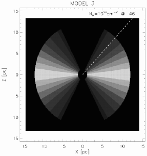
This model has the spatial density distribution shown in Figure 1c and is based on the work presented by Granato & Danese (gr_da (1994)). The density profile has an exponential dependency with the polar angle parameterised by a factor $\gamma$ (when $\phi<\phi_{c}$), and a power law dependancy with the radius parameterised by the index $\beta$:

$$\rho(r,\phi)=\rho_{\mbox{\scriptsize{eq}}}\ \left(\frac{r_{\mbox{\scriptsize{int}}}}{r}\right)^{\beta}\ e^{-\gamma\left|\sin(\phi)\right|}$$ (8)

where $\rho_{\mbox{\scriptsize{eq}}}$ is the inner torus density at the equatorial plane. The free parameters of the model are the opening angle $\phi_{{\mbox{\scriptsize{c}}}}$, $\gamma$ and $\beta$. The equation which describes the dependence of the column density with the line of sight is:

$$\begin{split}{\mbox{\scriptsize{\small{If}}}}&\quad 0\leq\phi<\phi_{\mbox{\scriptsize{c}}}\quad{\mbox{\scriptsize{\small{then,}}}}\quad N_{H}=N_{Hmax}\ e^{-\gamma\left|\sin(\phi)\right|}\\ {\mbox{\scriptsize{\small{If}}}}&\quad\phi_{\mbox{\scriptsize{c}}}\leq\phi\leq\pi/2\quad{\mbox{\scriptsize{\small{then,}}}}\quad N_{H}=N_{Hmin}\\ \end{split}$$ (9)

where $N_{Hmin}$ and $N_{Hmax}$ are fixed parameters at $10^{20}$ and $10^{25}$ cm^-2, respectively. The minimum value fixes $N_{H}$ at the poles and the maximum value fixes $N_{H}$ at the equatorial plane.

$$\begin{split}{\mbox{\scriptsize{\small{If}}}}&\quad\beta\neq 1\quad{\mbox{\scriptsize{\small{then,}}}}\quad N_{Hmax}=\rho_{\mbox{\scriptsize{eq}}}\ r_{\mbox{\scriptsize{int}}}^{\beta}\left(\frac{r_{\mbox{\scriptsize{out}}}^{1-\beta}-r_{\mbox{\scriptsize{int}}}^{1-\beta}}{1-\beta}\right)\\ {\mbox{\scriptsize{\small{If}}}}&\quad\beta=1\quad{\mbox{\scriptsize{\small{then,}}}}\quad N_{Hmax}=\rho_{\mbox{\scriptsize{eq}}}\ r_{\mbox{\scriptsize{int}}}\ln\left(\frac{r_{\mbox{\scriptsize{out}}}}{r_{\mbox{\scriptsize{int}}}}\right)\end{split}$$ (10)

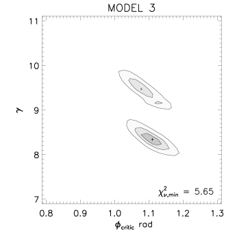
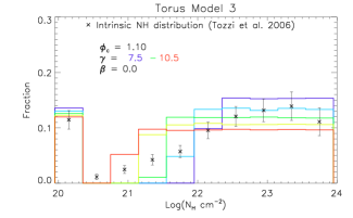
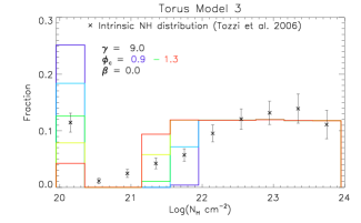
Searching for best fit parameters using the $\chi^{2}$ test, we obtain the results shown in Figure 2. This model gives a poor fit to the data ($\chi^{2}_{\nu,min}=5.65$), and is not able to reproduce the observed $N_{H}$ distribution between the first bin and those at $\la 10^{22}$ cm^-2 (Figure 3). The sharp gap seen at $N_{H}\lesssim 10^{21}cm^{-2}$ in the synthetic distributions corresponds to the transition produced when the line of sight no longer hits the torus ($\phi>\phi_{\mbox{\scriptsize{c}}}$). This dichotomy also affects the $\chi^{2}$ distribution where multiple minima are seen. Parameters between $57^{\mbox{\scriptsize{o}}}\lesssim\phi_{\mbox{\scriptsize{c}}}\lesssim 69^{\mbox{\scriptsize{o}}}$ and $8.0\lesssim\gamma\lesssim 10.0$ are found.

Simulations of the intrinsic $N_{H}$ distributions are shown in Figure 3. Changes in the value of $\phi_{\mbox{\scriptsize{c}}}$ affect the distribution over Type I sources only (i.e., for $N_{H}<10^{22}$ cm^-2), while $\gamma$ affects the number of sources at $N_{H}\approx 10^{21}$ cm^-2 and changes the fraction of Type II/I. The estimated intrinsic fraction of Compton Thick sources, using the best fit parameters, is about $26\%$.

When we compare our results with the work by Granato & Danese (gr_da (1994)), we find that our analysis can constrain $\phi_{c}$ (except for large $\gamma$ values), while Granato & Danese (gr_da (1994)) found that the spectral energy distribution for the reemission does not depend strongly on this parameter. On the other hand, we cannot constrain the outer radius, since this scale parameter is contained in $N_{Hmax}$ (Equation 10), and it could be easily adjusted to adopt any value (e.g. $>100$ pc, as found by Granato & Danese gr_da (1994)).

4.4 Model 4

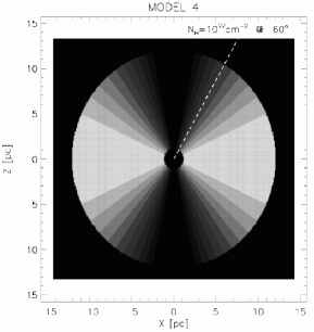
Many previous theoretical models trying to reproduce the IR reemission coming from the obscuring torus were based on continuous density distributions (as those presented in Models 1 to 3). Elitzur et al. (Elitzur (2003)) and Nenkova et al. (Nenkova (2002)) have developed the formalism to handle dust clumpiness and their results indicate that the inclusion of thick clouds may resolve the difficulties encountered by previous theoretical efforts trying to reproduce the observed IR spectral energy distributions of local AGNs. They have shown that some problems are naturally resolved if a clumpy media with $\sim 5-10$ clouds along radial rays (each one with $\tau_{V_{i}}\gtrsim 40$) is considered. The fundamental difference between clumpy and continuous density distributions is that radiation can propagate freely between different regions of an optically thick medium when it is clumpy, but not otherwise.

Following Elitzur et al. (Elitzur (2003)) we define the model given by Figure 1d, considering a spatially random cloud distribution per unit length given by:

$$n_{T}(r,\phi)=n_{{\mbox{\scriptsize{eq}}}}\left(\frac{r_{\mbox{\scriptsize{int}}}}{r}\right)^{\beta}\ e^{-\phi^{2}/\sigma^{2}}$$ (11)

where $n_{{\mbox{\scriptsize{eq}}}}$ is the inner number of clouds by unit length in the equatorial plane, $\sigma$ the half opening angle for the angular distribution, and $\beta$ the power law index describing the radial dependency. Integrating the last equation along the line of sight, we obtain the average number of clouds, $N_{T}$ as a function of the line of sight, parameterised by the angle $\phi$:

$$N_{T}(\phi)=N_{{\mbox{\scriptsize{eq}}}}\ e^{-\phi^{2}/\sigma^{2}}$$ (12)

where $N_{\mbox{\scriptsize{eq}}}$ is the average number of clouds along the equatorial plane:

$$\begin{split}{\mbox{\scriptsize{\small{If}}}}&\quad\beta\neq 1\quad{\mbox{\scriptsize{\small{then,}}}}\quad N_{{\mbox{\scriptsize{eq}}}}=n_{{\mbox{\scriptsize{eq}}}}\frac{r_{\mbox{\scriptsize{int}}}^{\beta}}{1-\beta}\left(r_{\mbox{\scriptsize{out}}}^{1-\beta}-r_{\mbox{\scriptsize{int}}}^{1-\beta}\right)\\ {\mbox{\scriptsize{\small{If}}}}&\quad\beta=1\quad{\mbox{\scriptsize{\small{then,}}}}\quad N_{{\mbox{\scriptsize{eq}}}}=n_{{\mbox{\scriptsize{eq}}}}r_{\mbox{\scriptsize{int}}}\ln\left(\frac{r_{\mbox{\scriptsize{out}}}}{r_{\mbox{\scriptsize{int}}}}\right)\\ \end{split}$$ (13)

Assuming $\tau_{V}=N_{T}\tau_{V_{i}}$, and considering Equation 1, we can estimate the Hydrogen column density dependency on the line of sight, as:

$$N_{H}(\phi)=N_{Hmax}\ e^{-\phi^{2}/\sigma^{2}}$$ (14)

The fixed parameter $N_{Hmax}$ constrains the optical depth, the number of clouds along the line of sight at the equatorial plane, and the parameter $\beta$:

$$N_{Hmax}=2.0\cdot 10^{21}N_{\mbox{\scriptsize{eq}}}\tau_{Vi}$$ (15)

If a certain value $\tau_{Vi}$ is assumed for the clumps, the only remaining free parameter for this distribution is $\sigma$. However, restricting $N_{T}$ to represent a discrete number of clouds and assuming a poissonian probability for the number of clouds along the line of sight, it is also possible to constrain the optical depth per cloud, $\tau_{Vi}$. In the case when the optical depth tends to zero but $N_{T}$ tend to infinity, the continuous case is recovered, where column densities are allowed to have any value. Note that Nenkova et al. (Nenkova (2002)) assumed $\tau_{V_{i}}=40$ to reproduce the IR reemission from the torus, implying a minimum column density of $8.0\cdot 10^{22}$ cm^-2. Clearly, smaller optical depths per cloud are necessary to explain the observed distribution of $N_{H}$. A work around this difficulty which would still be consistent with a large $\tau_{Vi}$ per cloud, is to assume that absorption by overdensities of diffuse material located in the outer regions or within the torus might be responsible for the smaller observed column densities.

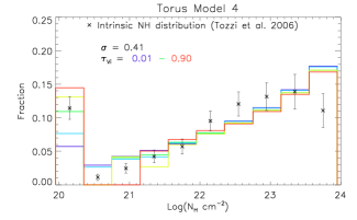
The best-fit values for $\sigma$ and $\tau_{Vi}$ are shown in Figure 2. Multiple minima in the $\chi^{2}$ distribution are found due to the cloud number discretization and the selected $N_{H}$ bin-size. Values between $22^{\mbox{\scriptsize{o}}}\lesssim\sigma\lesssim 25^{\mbox{\scriptsize{o}}}$ and $\tau_{Vi}\lesssim 0.8$ are preferred. Parameter $\sigma$ changes the number of objects at $N_{H}=10^{20}$ cm^-2 and at $N_{H}=10^{25}$ cm^-2, without altering significantly the intermediate values where a increasing slope in the synthetic distributions is seen. On the other hand, the optical depth per cloud creates a dichotomy between Type II and Type I objects, where the minimum value of $N_{H}$ is given by the optical depth of a single cloud.

From Figure 4, it is clear that this model gives the largest number of Compton Thick sources produced by lines of sights near the equatorial plane (approximately a fraction of $\sim 58\%$ using best fit parameters). On the other hand, if a lower $N_{Hmax}$ of $10^{24}$ cm^-2 is adopted, the gaussian angular dependency generates large discrepancies with the observed column densities.

When we compare our parameters with the results coming from the reemission treatment given by Elitzur et al. (Elitzur (2003)), we found that our typical Gaussian angular distributions are smaller than Elitzur’s values. In fact, they find a valid range of $\sigma=45^{\mbox{\scriptsize{o}}}\pm 15^{\mbox{\scriptsize{o}}}$. Also, their estimations for the number of clouds along the equatorial plane ($N_{\mbox{\scriptsize{eq}}}\approx 5-10$) correspond to a maximum column density of $\sim 10^{24}$ cm^-2 (see Equation 1), one order of magnitude smaller than our assumptions. In our models, since $N_{Hmax}=10^{25}$ cm^-2, the value of $N_{\mbox{\scriptsize{eq}}}$ depends on the assumed $\tau_{Vi}$.

Note that since $N_{H}\propto N_{T}$, this clumpy model requires a wide range for the number of clumps (at least $\sim 3$ orders of magnitude) to describe the wide range of observed $N_{H}$s.

5 Discussion

5.1 Torus Properties as a Function of Luminosity

The work of Barger et al. (Barger05 (2005)), based on a complete AGN sample at $z<1.2$, shows a dependency of the fraction of Type II/I AGN with luminosity. This observational evidence implies that our simple models, where the torus does not evolve with neither luminosity nor redshift, might not be an accurate representation.

Treister & Urry (Treister05 (2005)) found a simple explanation for Barger’s results assuming a Modified Unification Model, where the percentage of obscured AGNs varies linearly from 100% at $L_{X}=10^{42}$ erg sec^-1 to 0% at $L_{X}=3\cdot 10^{46}$ erg sec^-1. We can examine how this luminosity evolution would change our results for the torus models. Using the luminosity dependency for the fraction of Type II AGN determined by La Franca et al. (lafranca05 (2005)), we find that in the case of Model 1 (the one with the best statistical results), parameter $\gamma$, which is mostly responsible for the variations observed in this fraction, changes to $\approx 7.0$, $14$ and $23$ (fixing $R_{m}/R_{t}=1.1$) for the luminosity bins $10^{42-43}$, $10^{43-44}$ and $10^{44-45}$ erg sec^-1, respectively. These values take into account the observational incompleteness for the Type II population in La Franca’s X-Ray sample ($\sim$1/3 of the sources would not observed). Table 1 shows that our results give an estimate of $7.0\lesssim\gamma\lesssim 9.0$, roughly coinciding with $\gamma$ for the lowest and middle luminosity bins in La Franca’s sample.

Unfortunately, the current statistics of the observed $N_{H}$ distribution does not allow us to test such luminosity dependency. However, the number density of the most luminous sources is much smaller than those of low and intermediate luminosity, with fractions of 63%, 30%, and 7% for the $10^{42-43}$, $10^{43-44}$ and $10^{44-45}$ erg sec^-1 luminosity bins (integrating $L_{X}$ from $10^{42}$ to $10^{45}$ erg sec^-1 in the Ueda’s luminosity function). Therefore, the general $N_{H}$ distribution is clearly dominated for the less powerful (Seyfert like) AGN, for which the derived torus properties might be a good representation.

5.2 Column Densities Uncertainties

Our analysis is based on the distribution of the determined column densities. From this measurements, it is not possible to determine how far from the central source the absorption is produced. This implies that overdensities of gas located closer than the graphite sublimation radius will not have the assumed Gas-to-Dust ratio. This possibility is consistent with the extreme variability of the column density observed in the Seyfert galaxy NGC 1365 (Risaliti et al. Risaliti05 (2005)). Also, assuming higher metallicities gives a harder photoelectric absorption, increasing the estimation of the number of Type I sources. Finally, changing the parameter $R_{V}$ from $3.1$ to $5.0$ produces small differences in our results.

A spectroscopic analysis such as the one conducted by Tozzi et al. (tozzi (2006)) is essential to estimate the distribution of column densities since particular spectral features for each source can be present in the data. Broad band estimations, using $Hardness$ $Ratios$ are not precise enough and are highly affected by the template assumed for the X-Ray source. These uncertainties affect the best-fit model parameters, and the error bars for these estimations. We conclude that a direct fit to the spectral features is determinant at the time to describe the obscuring properties of the AGN population.

5.3 Torus Model Results

Recent IR observations have derived compact torus structures in nearby Seyfert II galaxies (Jaffe et al. jaffe (2004); Prieto et al. prieto (2004), prieto05 (2005); Swain et al. swain (2003)) in agreement with the sizes predicted for model 1, while for models 3 and 4 this physical scale can be freely adjusted.

It has been argued that a constant torus density distribution does not explain the reemission IR spectrum in AGN, but the inclusion of a clumpy medium solves this problem. Models 1 to 3 can be discretized using Equation 1, while adopting small optical depths per cloud allows predictions of Type I sources at $\la 10^{21}$ cm^-2, avoiding a large dichotomy between Type II and Type I objects (see Model 4 for details).

Exponential angular dependencies of the parameter $\rho$ (see Equation 1) allow smooth density decrements from the equatorial plane to the poles, so that a wide range of $N_{H}$ can be obtained, implying that Model 1 and 3 are the most favorable obscuring structures. On the other hand, radial dependencies for the models ($\beta\neq 0$) can shrink the effective torus radius, increasing the inner equatorial density, more according with dynamical simulations of a thick clumpy torus (see Beckert & Duschl be_du (2004)).

5.4 Highly absorbed sources

According to the X-Ray analysis of Seyfert II galaxies presented by Maiolino et al. (Maiolino (1998)), the number of Compton Thick sources represents a large fraction of the AGN population. In this work, the assumption of a maximum column density at $N_{H}=10^{25}$ cm^-2 allows us to estimate this highly absorbed population from our geometrical assumptions (see Figure 4). We roughly predict intrinsic Compton Thick source fractions of 27%, 3%, 26% and 58% for Model 1, 2, 3 and 4 respectively. Work by Tozzi et al. (tozzi (2006)) estimate a lower limit for the Compton Thick fraction of $\sim 10\%$ in the CDF-S, while Beckmann et al. (beckmann (2006)) find 4 Compton Thick sources of a total of 40 AGN observed with $INTEGRAL$ in the 20-40 keV energy range at $z\sim 0$. These values are somewhat smaller, but still consistent with predictions from Models 1 and 3 given the uncertainties involved.

6 Conclusions

1. Using the observed distribution of $N_{H}$ columns for AGNs in the CDF-S, we have constrained the geometry of the obscuring region present in AGNs. Four different torus geometries, based on previously proposed models (see Figure 1), have been explored. No luminosity or redshift dependency has been included in the torus modelling.

2. Results from our fit to the $N_{H}$ distribution are presented in Table 1 which shows the model parameter best-fit values. These results can be used to estimate physical properties of the torus, such as the inner and outer radius, and the density at the equatorial plane, as a function of the AGN luminosity.

3. Detailed analysis shows that a matter density profile ($\rho(\phi)$) with an exponential dependency in $\phi$, such as in Model 1 and 3, gives the best representation of the wide range of observed column densities (from $\sim 10^{20}$ cm^-2 to $\sim 10^{25}$ cm^-2). A constant density distribution (Model 2) requires very extended structures to recover the wide observed $N_{H}$ range (since $N_{H}\propto\Delta s$), not according with actual observations of local Seyfert galaxies where pc-scale torus-like structures have been detected. It also underestimates the fraction of Type II sources. A Gaussian angular dependency (Model 4), as in the clumpy model proposed by Nenkova et al. (Nenkova (2002)), results in a substantial overestimation of highly obscured sources. We also find that the optical depth for individual clumps, $\tau_{Vi}$, has to be $\sim 60$ times smaller than the value adopted by Nenkova to compute the torus IR reemission. We note that the clumpy torus treatment could also be applied to other model distributions using Equation 1 and a suitable value for $\tau_{Vi}$. Models 3 and 4 suffer of multiple $\chi^{2}$ minima caused by the dichotomy between Type I and Type II sources (given by the critical value of $\phi$ and the presence of at least 1 clump along the line of sight, respectively).

4. We therefore conclude that Model 1, a classical ‘donut shape’, is the best parameterization for the obscuring region around AGN. Since no luminosity dependency has been included in our modelling, the results can be regarded as a luminosity averaged parameterization of the torus, which is largely dominated by low and intermediate luminosity sources.

Figure 1: Geometrical matter density distributions assumed for the torus models. Figures a$)$, b$)$ c$)$ and d$)$ are based on the previous work by Treister et al. (Treister (2004)), Pier & Krolik (pi_kr92 (1992)), Granato & Danese (gr_da (1994)) and Nenkova et al. (Nenkova (2002)), respectively.

Figure 2: Best-fit parameters found for each model following Section 4. Contours represent 1, 2 and 3 $\sigma$ confidence limits. Note that for Model 1 $\beta=0.0$.

Figure 3: Comparison between the column densities of the observed $Chandra$ sources in the CDF-S field (crosses) and the best-fit results obtained from our modelling. For each model, two histograms are presented varying the range of interest of one parameter only.

Figure 4: Geometrical matter density distribution using best fit parameters for each model. Model 1: $R_{m}/R_{t}=1.14$, $\gamma=9.0$ and $\beta=0.0$; Model 2: $h/a=3.0$ and $b/a=350$; Model 3: $\phi_{c}=1.1$ and $\gamma=9.5$; Model 4: $\sigma=0.4$ and $\tau_{Vi}<<1$ (continuous case). The inner radius is set at 1.2 pc for all models, and an outer radius at 12 pc for models 3 and 4 (but adjustable for more compact structures). Different shades mean $\Delta\log(N_{H})=0.5$, starting from $10^{25}$ cm^-2 at the equatorial plane. The dashed line represents the line of sight that divides the Type I and the Type II sources. Note that Model 2 is shown at a different scale.