INJE-TP-06-04, astro-ph/0605684

Gauss-Bonnet braneworld and WMAP three year results

Brian M. Murray^a and Yun Soo Myung^a,b

^aInstitute of Theoretical Science, University of Oregon, Eugene, OR 97403-5203, USA
^bInstitute of Mathematical Sciences, Inje University, Gimhae 621-749, Korea

Abstract

We compare predictions for the spectral index and tensor-scalar ratio in models of patch inflation with the WMAP three year data. There are three cases of these models of inflation, which arise in the Gauss-Bonnet braneworld scenario: Gauss-Bonnet (GB), Randall-Sundrum (RS), and 4D general relativity (GR). We consider the large-field potential $V\propto\phi^{p}$ in both commutative and noncommutative spacetimes, and find that in the cases of the GB and GR patch cosmologies, the quadratic potential is observationally favored, while the quartic potential is ruled out in most patches. Strong noncommutative inflation is excluded in all cases because it leads to a blue-tilted scalar spectral index.

1 Introduction

In recent years there has been much interest in the phenomenon of localization of gravity proposed by Randall and Sundrum (RS) [1]. They assumed a three-brane with a positive tension embedded in 5D anti-de Sitter (AdS₅) spacetime, and were able to localize gravity on the brane by fine-tuning the brane tension to the bulk cosmological constant. Recently, several authors have studied the cosmological implications of braneworld scenarios. As would be expected, brane cosmology contains some important deviations from the Friedmann-Robertson-Walker cosmology [2].

At the same time, it is generally thought that curvature perturbations produced during inflation may be the origin of the inhomogeneity that is necessary to explain the anisotropy in the cosmic microwave background as well as the presence of large-scale structure. The WMAP first year results (WMAP1) [3], SDSS [4, 5], and other data lead to more constraints on cosmological models. As a result of combining these results from various observations, the ${\rm\Lambda}$CDM model has emerged in recent years as the standard model of cosmology. Moreover, these results coincide with the theoretical prediction of slow-roll inflation with a single inflaton field.

Recently, the WMAP three year results (WMAP3) [6] obtained values for the spectral index $n_{s}=0.951^{+0.015}_{-0.019}~{}(0.948^{+0.015}_{-0.018})$ and the tensor-scalar ratio $r<0.55~{}(0.28)$ for WMAP3 alone (WMAP3+SDSS) at the $2\sigma$ level. More recently, combined data including WMAP3, SDSS, Lyman-$\alpha$, SN Ia and galaxy clustering (combined DATA) indicated $n_{s}=0.965^{+0.012+0.025}_{-0.012-0.024}$ and $r<0.22$ [7]. It would appear that a red power spectrum with $n_{s}<1$ is favored, while a scale-invariant Harrison-Zel’dovich-Peebles (HZ) spectrum ($n_{s}=1,r=0$) is disfavored at the 2$\sigma$ level. The authors of [8], however, reported that the HZ spectrum is consistent with both WMAP3 and WMAP3+SDSS at the $2\sigma$ level. We use the combined DATA in this work due to the fact that the contours for WMAP3 and WMAP3+SDSS in Fig. 14 of Ref. [6] were incorrect [9, 8]. If one allows for a running spectral index $\alpha_{s}$, the fit to the WMAP3 data is slightly improved. The improvement, however, is not significant enough to require the running. Hence, we choose to neglect running ($\alpha_{s}\simeq 0$) for comparison with theoretical values. Importantly, it is shown that chaotic inflation with $V(\phi)\sim\phi^{2}$ fits the observations very well. It is certainly the case that the WMAP3 data with or without additional observations provides significant constraints on models of inflation and some models are ruled out at a high level of confidence [10].

If inflation occurs on the brane, one would expect that it provides us quite different results in the high-energy region [11]. Since the Gauss-Bonnet term significantly modifies the Friedmann equation at high-energy, its application to brane inflation has been studied widely in the literature [12]. Moreover, noncommutative spacetime naturally emerges in string theory, and although a realistic inflationary model has not yet been constructed in noncommutative spacetime, there is a toy model of noncommutative inflation  [13].

In this work, patch cosmological models that arise in the Gauss-Bonnet braneworld scenario are used to study brane inflation for large-field potentials in noncommutative spacetime. We use the leading-order theoretical predictions for the spectral index and tensor-scalar ratio to determine which patch models are consistent with the combined DATA.

The organization of this work is as follows. In section 2 we briefly review patch cosmology in noncommutative spacetime. We introduce large-field potentials, compute their theoretical values of $n_{s}$ and $r$, and compare these predictions with the observation data in section 3. Finally, we discuss our results in section 4.

2 Patch cosmological models

We start with the action for the Gauss-Bonnet braneworld scenario [12]:

$$S = \frac{1}{2\kappa^{2}_{5}}\int_{{\rm bulk}}d^{5}x\sqrt{-g_{5}}\Big{[}R-2\Lambda_{5}+\alpha\Big{(}R^{2}-4R_{\mu\nu}R^{\mu\nu}+R_{\mu\nu\rho\sigma}R^{\mu\nu\rho\sigma}\Big{)}\Big{]}$$ (1)

$$+ \int_{{\rm brane}}d^{4}x\sqrt{-g}\Big{[}-\lambda+{\cal L}_{{\rm matter}}\Big{]},$$

where $\Lambda_{5}=-3\mu^{2}(2-\beta)$ is the AdS₅ bulk cosmological constant, with the AdS₅ energy scale $\mu=1/\ell$. ${\cal L}_{{\rm matter}}$ is the matter lagrangian for the inflaton field. $\kappa^{2}_{5}=8\pi/m_{5}^{3}$ is the 5D gravitational coupling constant and $\kappa^{2}_{4}=8\pi/m_{{\rm Pl}}^{2}$ is the 4D coupling constant. The Gauss-Bonnet coupling $\alpha$ may be related to the string energy scale $g_{s}$ ($\alpha\simeq 1/8g_{s}$) when the Gauss-Bonnet term is considered to be the lowest-order stringy correction to the 5D gravity. $\lambda$ is the brane tension. Relations between these quantities are $\kappa^{2}_{4}/\kappa^{2}_{5}=\mu/(1+\beta)$ and $\lambda=2\mu(3-\beta)/\kappa_{5}^{2}$, where $\beta=4\alpha\mu^{2}\ll 1$. The RS case of $\mu=\kappa_{4}^{2}/\kappa_{5}^{2}$ is recovered for $\beta=0$ $(\alpha=0)$. We have to distinguish between the GB ($\beta\ll 1$, $\beta\not=0$) and RS ($\beta=0$) cases. The exact Friedmann-like equation is given by a complicated form,

$$2\mu\sqrt{1+\frac{H^{2}}{\mu^{2}}}\Big{[}3-\beta+2\beta\frac{H^{2}}{\mu^{2}}\Big{]}=\kappa_{5}^{2}(\rho+\lambda),$$ (2)

where as usual $H=\dot{a}/a$. We, however, use an effective Friedmann equation

$$H^{2}=\beta^{2}_{q}\rho^{q}.$$ (3)

Here $q$ is a patch parameter labeling different models, and $\beta_{q}^{2}$ is a corresponding factor with energy dimension $[\beta_{q}]=E^{1-2q}$. We call the above “patch cosmology,” and summarize the three different models and their parameters in Table 1.

Table 1: Three patch cosmological models and the values of the parameters that classify them. Here $m^{4}_{\alpha}=[8\mu^{2}(1-\beta)^{3}/\beta\kappa^{4}_{5}]^{1/2}$ is the GB energy scale.

model	$q~{}(\zeta_{q})$	$\beta^{2}_{q}$	acceleration $(\omega_{q}$)	$\rho$
GB	2/3 (1)	$(\kappa^{2}_{5}/16\alpha)^{2/3}$	$-1\leq\omega<0$	$\rho\gg m^{4}_{\alpha}$
RS	2  (2/3)	$\kappa^{2}_{4}/6\lambda$	$-1\leq\omega<-2/3$	$\lambda\ll\rho\ll m^{4}_{\alpha}$
GR	1  (1)	$\kappa_{4}^{2}/3$	$-1\leq\omega<-1/3$	$\rho\ll\lambda$

Before we proceed, we note that the Gauss-Bonnet braneworld affects inflation only when the Hubble parameter is much larger than the AdS scale ($H\gg\mu$). As a result, there are two patch models, the GB case with $q=2/3$ and the RS case with $q=2$. For $H\ll\mu$, one recovers the 4D general relativistic (GR) case with $q=1$.

On the brane, let us introduce an inflaton field $\phi$ whose equation is given by

$$\ddot{\phi}+3H\dot{\phi}=-V^{\prime},$$ (4)

where dot and prime denote the derivative with respect to time $t$ and $\phi$, respectively. The energy density and pressure are given by $\rho=\dot{\phi}^{2}/2+V$ and $p=\dot{\phi}^{2}/2-V$. From now on, we use the slow-roll formalism for inflation: an accelerating universe $(\ddot{a}>0)$ is driven by an inflaton slowly rolling down its potential toward a local minimum. Then Eqs. (3) and (4) take the approximate form

$$H^{2}\approx\beta^{2}_{q}V^{q},~{}\dot{\phi}\approx-V^{\prime}/3H.$$ (5)

These are the equations for the background. In order for an inflation to terminate and for the universe to transition to a radiation-dominated phase, there must be a slow-roll mechanism. To this end, it is conventional to introduce Hubble slow-roll parameters ($\epsilon,\delta$) and potential slow-roll parameters ($\epsilon^{q},\delta^{q}$),

$$\epsilon=-\frac{\dot{H}}{H^{2}}\approx\epsilon^{q}=\frac{q}{6\beta^{2}_{q}}\frac{(V^{\prime})^{2}}{V^{1+q}},~{}~{}\delta=\frac{1}{H\dot{\phi}}\frac{d^{2}\phi}{dt^{2}}\approx\delta^{q}=\frac{1}{3\beta^{2}_{q}}\Big{[}\frac{q}{2}\frac{(V^{\prime})^{2}}{V^{1+q}}-\frac{V^{\prime\prime}}{V^{q}}\Big{]}.$$ (6)

The slow-roll parameter $\epsilon^{q}\geq 0$ governs the equation of state $p=\omega_{q}\rho$ with $\omega_{q}=-1+2\epsilon^{q}/3q$. This implies that an accelerating expansion occurs only for $\epsilon^{q}<1~{}(\omega_{q}<-1+2/3q)$ [14]. $\epsilon^{q}=0~{}(\omega_{q}=-1)$ corresponds to de Sitter inflation. The end of inflation is determined by $\epsilon^{q}=1~{}(\omega_{q}=-1+2/3q)$. Hence, the allowed regions for acceleration (inflation) depend on $q$, as shown in Table 1. If one chooses an inflation potential $V$, then potential slow-roll parameters ($\epsilon^{q},\delta^{q}$) are determined explicitly.

Noncommutative inflation arises by imposing a realization of the $*$-algebra on the brane coordinates: $[\tau,x]=il_{s}^{2}$, where $\tau=\int adt$, $x$ is a comoving spatial coordinate, and $l_{s}=1/M_{s}$ is the string scale[13, 15, 16, 17]. By introducing the noncommutative parameter $\delta=(M_{s}/H)^{2}$, the noncommutative algebra induces a cutoff $k_{0}(\delta)$, which divides the space of comoving wavenumbers into two regions: the UV-commutative perturbations generated inside the Hubble horizon ($H\ll M_{s}$) and the IR-noncommutative perturbations generated outside the horizon ($H\gg M_{s}$). In this case the amplitude of scalar perturbations is given by [16]

$$A_{s}^{2}=\frac{9\beta^{6}_{q}}{25\pi^{2}}\frac{V^{3q}}{V^{\prime 2}}\Sigma^{2}(\delta),$$ (7)

where $\Sigma(\delta)$ is a function that includes noncommutative effects. The above amplitude is evaluated at horizon crossing in the UV-limit, and at the time when the perturbation with comoving wavenumber $k$ is generated in the IR-limit. To the lowest-order in the slow-roll parameters, we have

$$\frac{d\ln\Sigma^{2}}{d\ln k}=\tilde{\sigma}\epsilon^{q},$$ (8)

where $\tilde{\sigma}=\tilde{\sigma}(\delta)$ is a function of $\delta$ and $\dot{\tilde{\sigma}}={\cal O}(\epsilon^{q})$. Here we choose three cases in the far IR-limit: $\tilde{\sigma}=0$ (UV-commutative case), $\tilde{\sigma}=2$ ($\Sigma^{2}\sim\delta$), and $\tilde{\sigma}=6$ ($\Sigma^{2}\sim\delta^{3}$). $\tilde{\sigma}=2~{}(6)$ correspond to the weak (strong) noncommutative case.

Figure 1: The spectral index $n_{s}$ versus number of e-foldings $N$ for the commutative case $\tilde{\sigma}=0$. The red, green, and blue curves represents the GB, GR, and RS cases, respectively. Solid (long-dashed) lines denote the case of $p=2~{}(4)$. The short-dashed lines denote the 1$\sigma$ interval between 0.953 and 0.977, while the dotted lines show the 2$\sigma$ interval between 0.941 and 0.990 [7].

Figure 2: The tensor-scalar ratio $r$ versus number of e-foldings $N$, with parameter values and colorings as in Fig. 1. The short-dashed line denotes the 2$\sigma$ level of $r<0.22$ [7].

The $q$-spectral index is given by

$$n^{q}_{s}(k)=1-(4-\tilde{\sigma})\epsilon^{q}-2\delta^{q},$$ (9)

and the tensor-scalar ratio $r_{q}$ is given by

$$r_{q}=16\frac{\epsilon^{q}}{\zeta_{q}},$$ (10)

where $\zeta_{q}$ is given by Table 1. Note that $r_{q}$ is independent of the noncommutative parameter.

3 Inflation with large-field potentials

Figure 3: The spectral index $n_{s}$ versus the number of e-foldings $N$ for the weak noncommutative case $\tilde{\sigma}=2$. All other parameters, colors, and lines are as in Fig. 1.

Figure 4: The spectral index $n_{s}$ versus the number of e-foldings $N$ for the strong noncommutative case $\tilde{\sigma}=6$. All other parameters, colors, and lines are as in Fig. 1.

A single-field potential can be characterized by two energy scales: the height of potential $V_{0}$ corresponding to the vacuum energy density for inflation and the width of the potential $w$ corresponding to the change in the inflaton $\Delta\phi$ during inflation. In general, the potential can be expressed as $V=V_{0}f(\phi/w)$. Different potentials have different choices for the function $f$. The height $V_{0}$ is usually fixed by normalization so that $w$ is the only free parameter in the potential. Here we focus on the case of large-field potentials, $V^{LF}=V_{0p}\phi^{p}$ for comparison with the combined DATA. For $p=2$, $V_{02}=m^{2}/2$ is the case of a massive scalar, and for $p=4$, $V_{04}=\lambda/4$ is the case of a model with a self-coupling. In these cases, the potential slow-roll parameters are

$$\epsilon^{q}_{p} = {{qp}\over 2}\frac{1}{X},$$ (11)

$$\delta^{q}_{p} = {1\over 2}{(2-2p+qp)\over X},$$ (12)

where we have defined $X\equiv[(q-1)p+2]N+{{qp}\over 2}$. Substituting these expressions into Eqs. (9) and (10), we obtain the desired results for $n_{s}$ and $r$. In the leading-order calculation, the LF-spectral index in noncommutative spacetime is given by

$$n_{s}^{LF}=1-\frac{(3q-q\tilde{\sigma}/2-2)p+2}{X}.$$ (13)

The LF tensor-scalar ratio takes the form

$$r^{LF}=\frac{8qp}{\zeta_{q}}\frac{1}{X}.$$ (14)

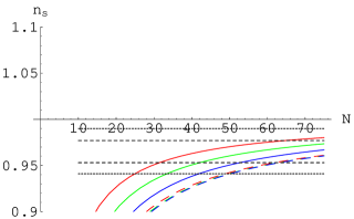
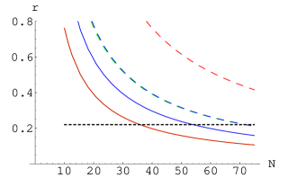
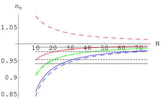
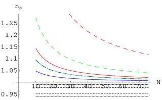
Fortunately, there are no additional free parameters for large-field potentials, once a choice has been made for the e-folding number $N$. See Figs. 1-4 for plots. In Fig. 1, three long-dashed curves are nearly the same for $p=4$, although the three solid ones are distinctive for $p=2$. In Fig. 2 consists only of monotonically decreasing functions of $N$. For $p=2$, the solid GB and GR curves are degenerate, while for $p=4$, the long-dashed GR and RS curves are degenerate. In Fig. 3 we plot $n_{s}$ for the weak noncommutative case $\tilde{\sigma}=2$. Here all curves are monotonically increasing functions except the case of $p=4$ in GB. The curves of GR for $p=2$ and $p=4$ are nearly the same, and the two cases of RS patch are even more degenerate. Finally, in Fig. 4 we plot $n_{s}$ for the strong noncommutative case $\tilde{\sigma}=6$. The curves for $p=2$ in GR and $p=4$ in RS are degenerate. Here all curves are monotonically decreasing functions above the 2$\sigma$ level, which shows that the strong noncommutativity leads to the blue-tilted scalar spectra with $n_{s}>1$ for large-field potentials.

Table 2: The spectral index $n_{s}$ and tensor-scalar ratio $r$ for three patch models (determined by $q$). We focus on the cases $N=50$ and $60$ to obtain theoretical values for large-field potentials $V=V_{0p}\phi^{p}$. Here we indicate $n_{s}=(\tilde{\sigma}=0,\tilde{\sigma}=2,\tilde{\sigma}=6)$.

Patch	$p$	$N=50$	$N=60$
GB	2	$n_{s}=(0.970,0.990,1.030),r=0.16$	$n_{s}=(0.975,0.992,1.025),r=0.13$
$(q=2/3)$	4	$n_{s}=(0.942,1.019,1.173),r=0.62$	$n_{s}=(0.952,1.016,1.145),r=0.52$
RS	2	$n_{s}=(0.950,0.970,1.010),r=0.24$	$n_{s}=(0.959,0.975,1.008),r=0.20$
$(q=2)$	4	$n_{s}=(0.941,0.967,1.020),r=0.32$	$n_{s}=(0.951,0.973,1.016),r=0.26$
GR	2	$n_{s}=(0.960,0.980,1.020),r=0.16$	$n_{s}=(0.967,0.983,1.017),r=0.13$
$(q=1)$	4	$n_{s}=(0.941,0.980,1.059),r=0.31$	$n_{s}=(0.951,0.984,1.049),r=0.26$

4 Discussion

Figure 5: Observational constraints ($1\sigma~{}(68\%$ C.L.) and $2\sigma~{}(95\%$ C.L.) contours) in the $n_{s}$-$r$ plane on large-field potentials for the GR patch. The theoretical values correspond to (a) $p=2$ (dots) with $N$=50, 60 and 70 (top to bottom) Three classes of (non)commutative inflation are at left ($\tilde{\sigma}=0$:black), center ($\tilde{\sigma}=2$:blue), and right ($\tilde{\sigma}=6$:green). (b) $p=4$ (squares) with $N$=60 and 70. Here $\tilde{\sigma}=6$ is absent.

Figure 6: Same contours in the $n_{s}$-$r$ plane as in Fig. 5. The theoretical values for the case of the GB patch correspond to $p=2$ (dots) with $N$=50, 60 and 70 (top to bottom). Two of (non)commutative inflation are at left ($\tilde{\sigma}=0$) and center ($\tilde{\sigma}=2$). The case of $\tilde{\sigma}=6,N=70$ appears at right. Note that $p=4$ is not present at this graph.

Figure 7: Same contours in the $n_{s}$-$r$ plane as in Fig. 5. The theoretical values for the case of the RS patch correspond to (a) $p=2$ (dots) with $N$=50, 60 and 70 (top to bottom). (b) $p=4$ (squares) with $N=60$ and 70. Three classes of (non)commutative inflation are at left ($\tilde{\sigma}=0$), center ($\tilde{\sigma}=2$), and right ($\tilde{\sigma}=6$).

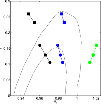
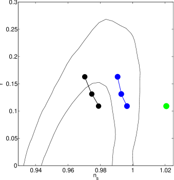
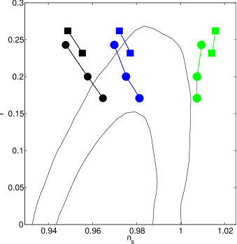
For large-field potentials, the spectral index $n_{s}$ and tensor-scalar ratio $r$ depend on the e-folding number $N$ only. This simplicity leads to strong constraints on large-field potentials. Further, combining the Gauss-Bonnet braneworld with large-field potentials provides even tighter constraints than for the GR case. It was shown with WMAP1 that the quartic potential $V=V_{04}\phi^{4}$ is under strong observation pressure (ruled out observationally) for GR and RS (GB) patches, while the quadratic potential $V=V_{02}\phi^{2}$ is inside the 1$\sigma$ bound for GR and GB patches for a range of e-folding number $50\leq N\leq 60$. This potential, however, is outside the 1$\sigma$ bound for RS patch. This is obtained from the likelihood analysis of $n_{s}$ and $r$ with the leading-order calculation for patch cosmological models [16].

The main feature of the combined DATA is the red-tilted scalar spectral index $n_{s}<1$ and the small tensor-scalar ratio $r<0.22$. We show the theoretical values of $n_{s}$ and $r$ for $N=50$ and 60 in Table 2. For $\tilde{\sigma}=2$, $p=4$ in GB and all cases of $\tilde{\sigma}=6$, we have blue-tilted scalar spectra with $n_{s}>1$. Also, in all cases $p=4$ leads to $r>0.22$, which is beyond the $2\sigma$ bound. In order to compare these values with the combined DATA, we should have nine $n_{s}$-$r$ figures with different contours, in order to take into account all possible combinations of $q$ and $\tilde{\sigma}$. As was shown in the figures constructed by the WMAP1 [16], however, these contours are similar except for a minor modification of the upper bound on $r$. Hence, we use Fig. 5 constructed for the $\tilde{\sigma}=0$ GR patch with the combined DATA [7] to plot all theoretical values of large-field potentials, instead of generating different contours for each combination of $q$ and $\tilde{\sigma}$.

We start with the GR patch with $\tilde{\sigma}=0$. The large-field potential $V\propto\phi^{p}$ is consistent with the combined DATA for $p=2$, and is marginally consistent with the WMAP3 alone for $p=4$ but ruled out by the WMAP3+SDSS [8]. In Fig. 5, we see that the quadratic potential is inside the $2\sigma$ contour, while the quartic potential is outside the $2\sigma$ contour for $50\leq N\leq 70$. Hence we find that the quartic potential is ruled out by the combined DATA [7]. The weak noncommutative case of $\tilde{\sigma}=2$ is favored for the observational compatibility of the quadratic potential, while the strong noncommutative case of $\tilde{\sigma}=6$ is disfavored. The quartic potential is marginally compatible for $\tilde{\sigma}=2$ and it is not allowed for $\tilde{\sigma}=6$. The authors of [16] argued that the quartic potential is rescued from the marginal rejection in the $\tilde{\sigma}=2$ GR case when using the WMAP1 data. However, it is not clear whether this is correct, since this case is on the border of the $2\sigma$ contour.

Now we are more on to the GB patch. When combined with the Gauss-Bonnet braneworld, it was recently shown that the GB patch may provide a successful cosmology [19]. The GB and GR patches provide nearly the same result for the quadratic potential according to the WMAP1  [16]. In Fig. 6 we see that the quartic potential is ruled out observationally for all $\tilde{\sigma}=0$, $2$ and $6$, while the quadratic potential is located near the $1\sigma$ bound for $\tilde{\sigma}=0$ and inside the $2\sigma$ bound for $\tilde{\sigma}=2$. However, it is outside the $2\sigma$ bound for the strong noncommutative case with $\tilde{\sigma}=6$. Hence the quadratic potential in GB patch is consistent with the combined DATA, as is similar to the GR case. At this stage we compare the RS patch with the combined DATA. As is shown in Fig. 7, the quartic potential is under strong observational pressure, similar to the GR case. The case of $\tilde{\sigma}=6$, $p=2$ is outside the $2\sigma$ bound, and the $\tilde{\sigma}=0$, $p=2$ and $\tilde{\sigma}=2$, $p=2$ cases are on the boundary of the $2\sigma$ contour.

On the other hand, we feel from Figs. 5 and 7 that the quartic potential might become marginally compatible in $\tilde{\sigma}=2$ GR and $\tilde{\sigma}=2$ RS patches. There is no significant difference between GR and RS patches even though the tensor-scalar ratio $r$ is slightly larger in RS than in GR. Then it would be premature to claim that the quartic potential is ruled out in the Gauss-Bonnet braneworld. In this case it is better to study the exact Friedmann equation (2) than the effective Friedmann equation (3). As an example, one may consider the passage of RS $\to$ GR $\to$ GB. Here the GR exists as the intermediate regime. In this case the quartic potential in GR patch might come within the $2\sigma$ bound  [20].

Finally, we wish to mention the inflation induced by tachyon field. It is known that the tensor-scalar ratio is smaller in the tachyon inflation than the scalar inflation irrespective of the kind of patch cosmologies. Hence we expect that this leads to the compatibility with the combined WMAP3. Further, the effect of noncommutativity could induce a blue-tilted spectrum with $n_{s}>1$ as is similar to the standard scalar field. However, we did not investigate the tachyon inflation because we focused on the standard scalar inflation in this work.

In conclusion, the quadratic potential is acceptable for GR and GB patches, while the quartic potential is ruled out by the combined DATA in most of patches. However, there is a possibility that the quartic potential is marginally compatible with the combined DATA in $\tilde{\sigma}=2$ GR and $\tilde{\sigma}=2$ RS patches. We note that the strong noncommutative inflation $\tilde{\sigma}=6$ is excluded because it leads to blue-tilted scalar spectra. A more thorough comparison of the combined DATA with (non)commutative patch models would necessarily involve computing all nine likelihood contours.

Acknowledgments

B. Murray was supported by the Department of Energy under DE-FG06-85ER40224. Y. Myung was supported by the Korea Research Foundation Grant (KRF-2005-013-C00018).

References

- [1] L. Randall and R. Sundrum, Phys. Rev. Lett. 83 (1999) 4690 [hep-th/9906064].
- [2] P. Binetruy, C. Deffayet and D. Langlois, Nucl. Phys. B565 (2000) 269 [hep-th/9905012]; P. Binetruy, C. Deffayet, U. Ellwanger, and D. Langlois, Phys. Lett. B477 (2000) 285 [hep-th/9910219].
- [3] H. V. Peiris et al, Astrophys. J. Suppl. 148 (2003) 213 [astro-ph/0302225]; C. L. Bennett et al, Astrophys. J. Suppl. 148 (2003) 1 [astro-ph/0302207]; D. N. Spergel et al, Astrophys. J. Suppl. 148 (2003) 175 [astro-ph/0302209].
- [4] M. Tegmark et al [SDSS collaboration], Phys. Rev. D 69 (2004) 103501 [astro-ph/0310723].
- [5] U. Seljak et al. [SDSS Collaboration], Phys. Rev. D 71 (2005) 103515 [arXiv:astro-ph/0407372].
- [6] D. N. Spergel et al., arXiv:astro-ph/0603449.
- [7] U. Seljak, A. Slosar and P. McDonald, arXiv:astro-ph/0604335.
- [8] W. H. Kinney, E. W. Kolb, A. Melchiorri and A. Riotto, arXiv:astro-ph/0605338.
- [9] A. Lewis, arXiv:astro-ph/0603753.
- [10] L. Alabidi and D. H. Lyth, arXiv:astro-ph/0603539; Q. G. Huang and M. Li, arXiv:astro-ph/0603782; Q. Shafi and V. N. Senoguz, arXiv:astro-ph/0603830; H. J. de Vega and N. G. Sanchez, arXiv:astro-ph/0604136; Q. G. Huang, M. Li and J. H. She, arXiv:hep-th/0604186; R. Easther and H. Peiris, arXiv:astro-ph/0604214; Q. G. Huang, arXiv:astro-ph/0605442.
- [11] R. Maartens, D. Wands, B. A. Bassett, and I. P. Heard, Phys. Rev. D 62 (2000) 041301 [hep-ph/9912464]; A. R. Liddle and A. N. Taylor, Phys. Rev. D 65 (2002) 041301 [astro-ph/0109412]; E. Ramirez and A. R. Liddle, Phys. Rev. D 69 (2004) 083522 [astro-ph/0309608]; S. Tsujikawa and A. R. Liddle, JCAP 0403 (2004) 001 [astro-ph/0312162]; G. Calcagni, Phys. Rev. D 69 (2004) 103508 [hep-ph/0402126]; Kyong Hee Kim, H. W. Lee, and Y. S. Myung, Phys. Rev. D 70 (2004) 027302 [hep-th/0403210]; G. Huey and J. E. Lidsey, Phys. Lett. B 514 (2001) 217 [astro-ph/0104006]; G. Huey and J. E. Lidsey, Phys. Rev. D 66 (2002) 043514 [astro-ph/0205236]. D. Seery and A. Taylor, Phys. Rev. D 71 (2005) 063508 [arXiv:astro-ph/0309512]. G. Calcagni, JCAP 0311 (2003) 009 [hep-ph/0310304]; G. Calcagni, JCAP 0406 (2004) 002 [hep-ph/0312246]; E. J. Copeland and O. Seto, Phys. Rev. D 72 (20025) 023506 [hep-ph/0505149].
- [12] J. F. Dufaux, J. E. Lidsey, Maartens, and M. Sami, Phys. Rev. D 70 (2004) 083525 [hep-th/0404161]. G. Calcagni, Phys. Rev. D 70 (2004) 103525 [hep-th/0406006]; S. Tsujikawa, M. Sami, and R. Maartens, Phys. Rev. D 70 (2004) 063525 [astro-ph/0406078]; K. H. Kim and Y. S. Myung, Int. J. Mod. Phys. D 14 (2005) 1813 [arXiv:astro-ph/0406387]; M. Sami, N. Savchenko and A. Toporensky, Phys. Rev. D 70 (2004) 123528 [arXiv:hep-th/0408140].
- [13] R. Brandenberger and P. M. Ho, Phys. Rev. D 66 (2002) 023517 [AAPPS Bull. 12N1 (2002) 10] [arXiv:hep-th/0203119].
- [14] W. H. Kinney, arXiv:astro-ph/0406670.
- [15] Q. G. Huang and M. Li, JHEP 0306 (2003) 014 [arXiv:hep-th/0304203]; Q. G. Huang and M. Li, JCAP 0311 (2003) 001 [arXiv:astro-ph/0308458]; Q. G. Huang and M. Li, Nucl. Phys. B 713 (2005) 219 [arXiv:astro-ph/0311378].
- [16] G. Calcagni and S. Tsujikawa, Phys. Rev. D 70 (2004) 103514 [astro-ph/0407543].
- [17] H. s. Kim, G. S. Lee and Y. S. Myung, Mod. Phys. Lett. A 20 (2005) 271 [arXiv:hep-th/0402018]. Hungsoo Kim, G. S. Lee, H. W. Lee, and Y. S. Myung, Phys. Rev. D 70 (2004) 043521 [hep-th/0402198]; Y. S. Myung, Phys. Lett. B 601 (2004) 1 [hep-th/0407066]; X. Zhang and F. Q. Wu, Phys. Lett. B 638 (2006) 396[arXiv:astro-ph/0604195].
- [18] V. Sahni, M. Sami, and T. Souradeep, Phys. Rev. D 65 (2002) 023518 [arXiv:gr-qc/0105121].
- [19] G. Panotopoulos, arXiv:hep-ph/0511040.
- [20] M Sami and V. Sahni, Phys. Rev. D 70 (2004) 083513 [arXiv:hep-th/0402086].