Diffraction-Based Sensitivity Analysis of Apodized Pupil Mapping Systems

Abstract

Pupil mapping is a promising and unconventional new method for high contrast imaging being considered for terrestrial exoplanet searches. It employs two (or more) specially designed aspheric mirrors to create a high-contrast amplitude profile across the telescope pupil that does not appreciably attenuate amplitude. As such, it reaps significant benefits in light collecting efficiency and inner working angle, both critical parameters for terrestrial planet detection. While much has been published on various aspects of pupil mapping systems, the problem of sensitivity to wavefront aberrations remains an open question. In this paper, we present an efficient method for computing the sensitivity of a pupil mapped system to Zernike aberrations. We then use this method to study the sensitivity of a particular pupil mapping system and compare it to the concentric-ring shaped pupil coronagraph. In particular, we quantify how contrast and inner working angle degrade with increasing Zernike order and rms amplitude. These results have obvious ramifications for the stability requirements and overall design of a planet-finding observatory.

1 Introduction

The impressive discoveries of large extrasolar planets over the past decade have inspired widespread interest in finding and directly imaging Earth-like planets in the habitable zones of nearby stars. In fact, NASA has plans to launch two space telescopes to accomplish this, the Terrestrial Planet Finder Coronagraph (TPF-C) and the Terrestrial Planet Finder Interferometer (TPF-I), while the European Space Agency is planning a similar multi-satellite mission called Darwin. These missions are currently in the concept study phase. In addition, numerous ground-based searches are proceeding using both coronagraphic and interferometric approaches.

Direct imaging of Earth-like extrasolar planets in the habitable zones of Sun-like stars poses an extremely challenging problem in high-contrast imaging. Such a star will shine $10^{10}$ times more brightly than the planet. And, if we assume that the star-planet system is $10$ parsecs from us, the maximum separation between the star and the planet will be roughly $0.1$ arcseconds.

Design Concepts for TPF-C. For TPF-C, for example, the current baseline design involves a traditional Lyot coronagraph consisting of a modern 8th-order occulting mask (see, e.g., Kuchner et al. (2004)) attached to the back end of a Ritchey-Chretien telescope having an $8$m by $3.5$m elliptical primary mirror. Alternative innovative back-end designs still being considered include shaped pupils (see, e.g., Kasdin et al. (2003) and Vanderbei et al. (2004)), a visible nuller (see, e.g., Shao et al. (2004)) and pupil mapping (see, e.g., Guyon (2003) where this technique is called phase-induced amplitude apodization or PIAA). By pupil mapping we mean a system of two lenses, or mirrors, that takes a flat input field at the entrance pupil and produce an output field that is amplitude modified but still flat in phase (at least for on-axis sources).

The Pupil Mapping Concept. The pupil mapping concept has received considerable attention recently because of its high throughput and small effective inner working angle (IWA). These benefits could potentially permit more observations over the mission lifetime, or conversely, a smaller and cheaper overall telescope. As a result, there have been numerous studies over the past few years to examine the performance of pupil mapping systems. In particular, Guyon (2003); Traub and Vanderbei (2003); Vanderbei and Traub (2005); Guyon et al. (2005) derived expressions for the optical surfaces using ray optics. However, these analyses made no attempt to provide a complete diffraction through a pupil mapping system. More recently, Vanderbei (2006) provided a detailed diffraction analysis. Unfortunately, this analysis showed that a pupil mapping system, in its simplest and most elegant form, cannot achieve the required $10^{-10}$ contrast; the diffraction effects from the pupil mapping systems themselves are so detrimental that contrast is limited to $10^{-5}$. In Guyon et al. (2005) and Pluzhnik et al. (2006), a hybrid pupil mapping system was proposed that combines the pupil mapping mirrors with a modest apodization of oversized entrance and exit pupils. This combination does indeed achieve the needed high-contrast point spread function (PSF). In this paper, we call such systems apodized pupil mapping systems.

A second problem that must be addressed is the fact that a simple two-mirror (or two-lens) pupil mapping system introduces non-constant angular magnification for off-axis sources (such as a planet). In fact, the off-axis magnification for light passing through a small area of the exit pupil is directly proportional to the amplitude amplification in that small area. For systems in which the exit amplitude amplification is constant, the magnification is also constant. But, for high-contrast imaging, we are interested in amplitude profiles that are far from constant. Hence, off-axis sources do not form images in a formal sense (the ”images” are very distorted.) Guyon (2003) proposed an elegant solution to this problem. He suggested using this system merely as a mechanism for concentrating (on-axis) starlight in an image plane. He then proposed that an occulter be placed in the image plane to remove the starlight. All other light, such as the distorted off-axis planet light, would be allowed to pass through the image plane. On the back side would be a second, identical pupil mapping system (with the apodizers removed), that would “umap” the off-axis beam and thus remove the distortions introduced by the first system (except for some beam walk—see Vanderbei and Traub (2005)).

Sensitivity Analysis. What remains to be answered is how apodized pupil mapping behaves in the presence of optical aberrations. It is essential that contrast be maintained during an observation, which might take hours during which the wavefront will undoubtedly suffer aberration due to the small dynamic perturbations of the primary mirror. An understanding of this sensitivity is critical to the design of TPF-C or any other observatory. In Green et al. (2004), a detailed sensitivity analysis is given for shaped pupils and various Lyot coronagraphs (including the $8$th-order image plane mask introduced in Kuchner et al. (2004)). Both of these design approaches achieve the needed sensitivity for a realizable mission. So far, however, no comparable study has been done for apodized pupil mapping. One obstacle to such a study is the considerable computing power required to do a full 2-D diffraction simulation.

Aberrations Given by Zernike Polynomials. In this paper, we present an efficient method for computing the effects of wavefront aberrations on apodized pupil mapping. We begin with a brief review of the design of apodized pupil mapping systems in Section 2. We then present in Section 3 a semi-analytical approach to computing the PSF of systems such as pupil-mapping and concentric rings in the presence of aberrations represented by Zernike polynomials. For such aberrations, it is possible to integrate analytically the integral over azimuthal angle, thereby reducing the computational problem from a double integral to a single one, eliminating the need for massive computing power.

In Section 4, we present the sensitivity results for an apodized pupil mapping system and a concentric ring shaped pupil coronagraph, and compare the results.

2 Review of Pupil Mapping and Apodization

In this section, we review the apodized pupil mapping approach and introduce the specific system that we study in subsequent sections. It should be noted that this apodized pupil mapping design may not be the best possible. Rather, it is merely an example of such a system that achieves high contrast. Other examples can be found in the recent paper by Pluzhnik et al. (2006). Our aim in this paper is not to identify the best such system. Instead, our aim is to develop tools for carrying a full diffraction analysis of any apodized pupil mapping system.

2.1 Pupil Mapping via Ray Optics

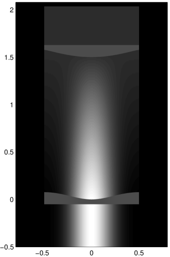
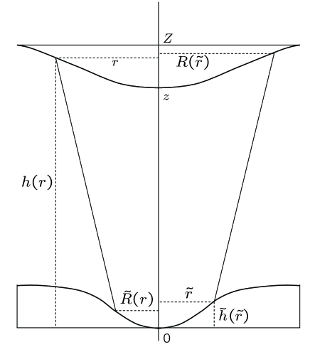
Figure 1: Pupil mapping via a pair of properly figured lenses. Light travels from top to bottom.

We begin by summarizing the ray-optics description of pure pupil mapping. An on-axis ray entering the first pupil at radius $r$ from the center is to be mapped to radius $\tilde{r}=\tilde{R}(r)$ at the exit pupil (see Figure 1). Optical elements at the two pupils ensure that the exit ray is parallel to the entering ray. The function $\tilde{R}(r)$ is assumed to be positive and increasing or, sometimes, negative and decreasing. In either case, the function has an inverse that allows us to recapture $r$ as a function of $\tilde{r}$: $r=R(\tilde{r})$. The purpose of pupil mapping is to create nontrivial amplitude profiles. An amplitude profile function $A(\tilde{r})$ specifies the ratio between the output amplitude at $\tilde{r}$ to the input amplitude at $r$ (in a pure pupil-mapping system the input amplitude is constant). Vanderbei and Traub (2005) showed that for any desired amplitude profile $A(\tilde{r})$ there is a pupil mapping function $R(\tilde{r})$ that achieves it (in a ray-optics sense). Specifically, the pupil mapping is given by

$$R(\tilde{r})=\pm\sqrt{\int_{0}^{\tilde{r}}2A^{2}(s)sds}.$$ (1)

Furthermore, if we consider the case of a pair of lenses that are planar on their outward-facing surfaces, then the inward-facing surface profiles, $h(r)$ and $\tilde{h}(\tilde{r})$, that are required to obtain the desired pupil mapping are given by the solutions to the following ordinary differential equations:

$$\frac{\partial h}{\partial r}(r)=\frac{r-\tilde{R}(r)}{|n-1|\sqrt{z^{2}+\frac{n+1}{n-1}(r-\tilde{R}(r))^{2}}},\qquad h(0)=z,$$ (2)

and

$$\frac{\partial\tilde{h}}{\partial\tilde{r}}(\tilde{r})=\frac{R(\tilde{r})-\tilde{r}}{|n-1|\sqrt{\phantom{\tilde{|}}z^{2}+\frac{n+1}{n-1}(R(\tilde{r})-\tilde{r})^{2}}},\qquad\tilde{h}(0)=0.$$ (3)

Here, $n\neq 1$ is the refractive index and $z$ is the distance separating the centers ($r=0$, $\tilde{r}=0$) of the two lenses.

Let $S(r,\tilde{r})$ denote the distance between a point on the first lens surface $r$ units from the center and the corresponding point on the second lens surface $\tilde{r}$ units from its center. Up to an additive constant, the optical path length of a ray that exits at radius $\tilde{r}$ after entering at radius $r=R(\tilde{r})$ is given by

$$Q_{0}(\tilde{r})=S(R(\tilde{r}),\tilde{r})+|n|(\tilde{h}(\tilde{r})-h(R(\tilde{r}))).$$ (4)

Vanderbei and Traub (2005) showed that, for an on-axis source, $Q_{0}(\tilde{r})$ is constant and equal to $-(n-1)|z|$.

2.2 High-Contrast Amplitude Profiles

If we assume that a collimated beam with amplitude profile $A(\tilde{r})$ such as one obtains as the output of a pupil mapping system is passed into an ideal imaging system with focal length $f$, the electric field $E(\rho)$ at the image plane is given by the Fourier transform of $A(\tilde{r})$:

$$E(\xi,\eta)=\frac{E_{0}}{\lambda if}e^{\pi i\frac{\xi^{2}+\eta^{2}}{\lambda f}}\int_{-\infty}^{\infty}\int_{-\infty}^{\infty}e^{-2\pi i\frac{\tilde{x}\xi+\tilde{y}\eta}{\lambda f}}A(\sqrt{\tilde{x}^{2}+\tilde{y}^{2}})d\tilde{y}d\tilde{x}.$$ (5)

Here, $E_{0}$ is the input amplitude which, unless otherwise noted, we take to be unity. Since the optics are azimuthally symmetric, it is convenient to use polar coordinates. The amplitude profile $A$ is a function of $\tilde{r}=\sqrt{\tilde{x}^{2}+\tilde{y}^{2}}$ and the image-plane electric field depends only on image-plane radius $\rho=\sqrt{\xi^{2}+\eta^{2}}$:

$$E(\rho) = \frac{1}{\lambda if}e^{\pi i\frac{\xi^{2}+\eta^{2}}{\lambda f}}\int_{0}^{\infty}\int_{0}^{2\pi}e^{-2\pi i\frac{\tilde{r}\rho}{\lambda f}\cos(\theta-\phi)}A(\tilde{r})\tilde{r}d\theta d\tilde{r}$$ (6)

$$= \frac{2\pi}{\lambda if}e^{\pi i\frac{\xi^{2}+\eta^{2}}{\lambda f}}\int_{0}^{\infty}J_{0}\left(-2\pi\frac{\tilde{r}\rho}{\lambda f}\right)A(\tilde{r})\tilde{r}d\tilde{r}.$$ (7)

The point-spread function (PSF) is the square of the electric field:

$$\mbox{Psf}(\rho)=|E(\rho)|^{2}.$$ (8)

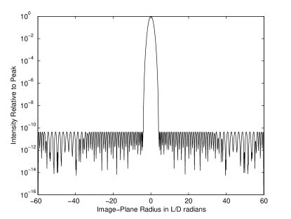
Figure 2: Left. An amplitude profile providing contrast of $10^{-10}$ at tight inner working angles. Right. The corresponding on-axis point spread function.

For the purpose of terrestrial planet finding, it is important to construct an amplitude profile for which the PSF at small nonzero angles is ten orders of magnitude reduced from its value at zero. A paper by Vanderbei et al. (2003a) explains how these functions are computed as solutions to certain optimization problems. The high-contrast amplitude profile used in the rest of this paper is shown in Figure 2.

2.3 Apodized Pupil Mapping Systems

Vanderbei (2006) showed that pure pupil mapping systems designed for contrast of $10^{-10}$ actually achieve much less than this due to harmful diffraction effects that are not captured by the simple ray tracing analysis outlined in the previous section. For most systems of practical real-world interest (i.e., systems with apertures of a few inches and designed for visible light), contrast is limited to about $10^{-5}$. Vanderbei (2006) considered certain hybrid designs that improve on this level of performance but none of the hybrid designs presented there completely overcame this diffraction-induced contrast degradation.

In this section, we describe an apodized pupil mapping system that is somewhat more complicated than the designs presented in Vanderbei (2006). This hybrid design, based on ideas proposed by Olivier Guyon and Eugene Pluzhnik (see Pluzhnik et al. (2006)), involves three additional components. They are

1. a preapodizer $A_{0}$ to soften the edge of the first lens/mirror so as to minimize diffraction effects caused by hard edges,

2. a postapodizer to smooth out low spatial frequency ripples produced by diffraction effects induced by the pupil mapping system itself, and

3. a backend phase shifter to smooth out low spatial frequency ripples in phase.

Note that the backend phase shifter can be built into the second lens/mirror. There are several choices for the preapodizer. For this paper, we choose Eqs. (3) and (4) in Pluzhnik et al. (2006) for our pre-apodizer:

$$A_{0}(r)=\frac{A(r)(1+\beta)}{A(r)+\beta A_{\mathrm{max}}},$$

where $A_{\mathrm{max}}$ denotes the maximum value of $A(r)$ and $\beta$ is a scalar parameter, which we take to be $0.1$. It is easy to see that

• $A(r)/A_{\mathrm{max}}\leq A_{0}(r)\leq 1$ for all $r$,

• $A_{0}(r)$ approaches $1$ as $A(r)$ approaches $A_{\mathrm{max}}$, and

• $A_{0}(r)$ approaches $0$ as $A(r)$ approaches $0$.

Incorporating a post-apodizer introduces a degree of freedom that is lacking in a pure pupil mapping system. Namely, it is possible to design the pupil mapping system based on an arbitrary amplitude profile and then convert this profile to a high-contrast profile via an appropriate choice of backend apodizer. We have found that a simple Gaussian amplitude profile that approximately matches a high-contrast profile works very well. Specifically, we used

$$A_{\mathrm{pupmap}}(\tilde{r})=3.35e^{-22(\tilde{r}/\tilde{a})^{2}},$$

where $\tilde{a}$ denotes the radius of the second lens/mirror.

The backend apodization is computed by taking the actual output amplitude profile as computed by a careful diffraction analysis, smoothing it by convolution with a Gaussian distribution, and then apodizing according to the ratio of the desired high-contrast amplitude profile $A(\tilde{r})$ divided by the smoothed output profile. Of course, since a true apodization can never intensify a beam, this ratio must be further scaled down so that it is nowhere greater than unity. The Gaussian convolution kernel we used has mean zero and standard deviation $\tilde{a}/\sqrt{100,000}$.

The backend phase modification is computed by a similar smoothing operation applied to the output phase profile. Of course, the smoothed output phase profile (measured in radians) must be converted to a surface profile (having units of length). This conversion requires us to assume a certain specific wavelength. As a consequence, the resulting design is correct only at one wavelength. The ability of the system to achieve high contrast degrades as one moves away from the design wavelength.

2.4 Star Occulter and Reversed System

It is important to note that the PSFs in Figure 2 correspond to a bright on-axis source (i.e., a star). Off-axis sources, such as faint planets, undergo two effects in a pupil mapping system that differ from the response of a conventional imaging system: an effective magnification and a distortion. These are explained in detail in Vanderbei and Traub (2005) and Traub and Vanderbei (2003). The magnification, in particular, is due to an overall narrowing of the exit pupil as compared to the entrance pupil. It is this magnification that provides pupil mapped systems their smaller effective inner working angle. The techniques in Section 3 will allow us to compute the exact off-axis diffraction pattern of an apodized pupil mapped coronagraph and thus to see these effects.

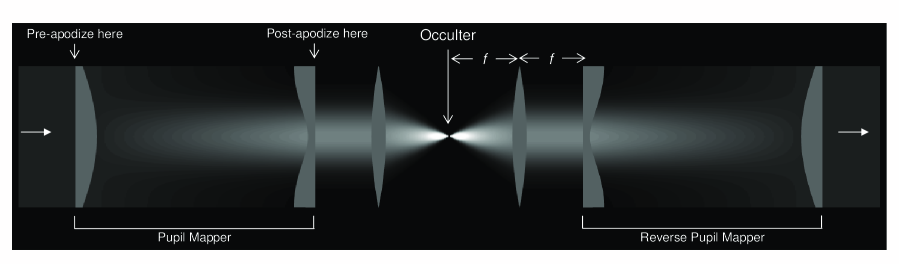
Figure 3: The full pupil mapping system includes: a pair of lenses to shape the amplitude into a prolate-spheroidal-like amplitude profile, a focusing lens that concentrates the on-axis starlight into a small central lobe where a (not-depicted) occulter can block this light, followed by a recollimating lens and finally a reverse pupil mapping system that reforms the pupil with the starlight removed but any planet light (if present) intact. This final pupil is then fed a final focusing element (not shown) to form an image of off-axis sources.

While the effective magnification of a pupil mapping system results in an inner working angle advantage of about a factor of two, it does not produce high-quaity diffraction limited images of off-axis sources because of the distortion inherent in the system. Guyon (2003) proposed the following solution to this problem. He suggested using this system merely as a mechanism for concentrating (on-axis) starlight in an image plane. He then proposed that an occulter be placed in the image plane to remove the starlight. All other light, such as the distorted off-axis planet light, would be allowed to pass through the image plane. On the back side would be a second, identical pupil mapping system (with the apodizers removed), that would “umap” the off-axis beam and thus remove the distortions introduced by the first system (except for some beam walk—see Vanderbei and Traub (2005)). A schematic of the full system (without the occulter) is shown in Figure 3. Note that we have spaced the lenses one focal length from the flat sides of the two lenses. As noted in Vanderbei and Traub (2005), such a spacing guarantees that these two flat surfaces form a conjugate pair of pupils.

3 Diffraction Analysis

In Vanderbei (2006), it was shown that a simple Fresnel analysis is inadequate for validating the high-contrast imaging capabilities we seek. Hence, a more accurate approximation was presented. In this section, we give a similar but slightly different approximation that is just as effective for studying pupil mapping but is better suited to the full system we wish to analyze.

3.1 Propagation of General Wavefronts

The goal of this section is to derive an integral that describes how to propagate a scalar electric field from one plane perpendicular to the direction of propagation to another parallel plane positioned downstream of the first. We assume that the electric field passes through a lens at the first plane, then propagates through free space until reaching a second lens at the second plane through which it passes. In order to cover the apodized pupil mapping case discussed in the previous section, we allow both the entrance and exit fields to be apodized.

Suppose that the input field at the first plane is $E_{\mathrm{in}}(x,y)$. Then the electric field at a particular point on the second plane can be well-approximated by superimposing the phase-shifted waves from each point across the entrance pupil (this is the well-known Huygens-Fresnel principle—see, e.g., Section 8.2 in Born and Wolf (1999)). If we assume that the two lenses are given by radial “height” functions $h(r)$ and $\tilde{h}(\tilde{r})$, then we can write the exit field as

$$E_{\mathrm{out}}(\tilde{x},\tilde{y})=A_{\mathrm{out}}(\tilde{r})\int_{-\infty}^{\infty}\int_{-\infty}^{\infty}\frac{1}{\lambda iQ(\tilde{x},\tilde{y},x,y)}e^{2\pi iQ(\tilde{x},\tilde{y},x,y)/\lambda}A_{\mathrm{in}}(r)E_{\mathrm{in}}(x,y)dydx,$$ (9)

where

$$Q(\tilde{x},\tilde{y},x,y)=\sqrt{(x-\tilde{x})^{2}+(y-\tilde{y})^{2}+(h(r)-\tilde{h}(\tilde{r}))^{2}}+n(Z-h(r)+\tilde{h}(\tilde{r}))$$ (10)

is the optical path length, $Z$ is the distance between the planar lens surfaces, $A_{\mathrm{in}}(r)$ denotes the input amplitude apodization at radius $r$, $A_{\mathrm{out}}(\tilde{r})$ denotes the output amplitude apodization at radius $\tilde{r}$, and where, of course, we have used $r$ and $\tilde{r}$ as shorthands for the radii in the entrance and exit planes, respectively.

As before, it is convenient to work in polar coordinates:

$$E_{\mathrm{out}}(\tilde{r},\tilde{\theta})=A_{\mathrm{out}}(\tilde{r})\int_{0}^{\infty}\int_{0}^{2\pi}\frac{1}{\lambda iQ(\tilde{r},r,\theta-\tilde{\theta})}e^{2\pi iQ(\tilde{r},r,\theta-\tilde{\theta})/\lambda)}A_{\mathrm{in}}(r)E_{\mathrm{in}}(r,\theta)rd\theta dr,$$ (11)

where

$$Q(\tilde{r},r,\theta)=\sqrt{r^{2}-2r\tilde{r}\cos\theta+\tilde{r}^{2}+(h(r)-\tilde{h}(\tilde{r}))^{2}}+n(Z-h(r)+\tilde{h}(\tilde{r})).$$ (12)

For numerical tractability, it is essential to make approximations so that the integral over $\theta$ can be carried out analytically, thereby reducing the double integral to a single one. To this end, we need to make an appropriate approximation to the square root term:

$$S=\sqrt{r^{2}-2r\tilde{r}\cos\theta+\tilde{r}^{2}+(h(r)-\tilde{h}(\tilde{r}))^{2}}.$$ (13)

A simple crude approximation is adequate for the $1/Q(\tilde{r},r,\theta-\tilde{\theta})$ amplitude-reduction factor in Eq. (11). We approximate this factor by the constant $1/Z$.

The $Q(\tilde{r},r,\theta-\tilde{\theta})$ appearing in the exponential must, on the other hand, be treated with care. The classical Fresnel approximation is to replace $S$ by the first two terms in a Taylor series expansion of the square root function about $(h(r)-\tilde{h}(\tilde{r}))^{2}$. As we already mentioned, this approximation is too crude. It is critically important that the integrand be exactly correct when the pair $(r,\tilde{r})$ correspond to rays of ray optics. Here is a method that does this. First, we add and subtract $S(\tilde{r},r,0)$ from $Q(\tilde{r},r,\theta)$ in Eq. (11) to get

$$Q(\tilde{r},r,\theta-\tilde{\theta}) = S(\tilde{r},r,\theta-\tilde{\theta})-S(\tilde{r},r,0)+S(\tilde{r},r,0)+|n|\left(\tilde{h}(\tilde{r})-h(r)\right)$$ (14)

$$= \frac{S(\tilde{r},r,\theta-\tilde{\theta})^{2}-S(\tilde{r},r,0)^{2}}{S(\tilde{r},r,\theta-\tilde{\theta})+S(\tilde{r},r,0)}+S(\tilde{r},r,0)+|n|\left(\tilde{h}(\tilde{r})-h(r)\right)$$

$$= \frac{r\tilde{r}-r\tilde{r}\cos(\theta-\tilde{\theta})}{(S(\tilde{r},r,\theta-\tilde{\theta})+S(\tilde{r},r,0))/2}+S(\tilde{r},r,0)+|n|\left(\tilde{h}(\tilde{r})-h(r)\right).$$

So far, these calculations are exact. The only approximation we now make is to replace $S(\tilde{r},r,\theta-\tilde{\theta})$ in the denominator of Eq. (14) with $S(\tilde{r},r,0)$ so that the denominator becomes just $S(\tilde{r},r,0)$. Putting this all together, we get a new approximation, which we refer to as the S-Huygens approximation:

$$E_{\mathrm{out}}(\tilde{r},\tilde{\theta}) \approx \frac{A_{\mathrm{out}}(\tilde{r})}{\lambda iZ}\int_{0}^{\infty}K(r,\tilde{r})\int_{0}^{2\pi}e^{2\pi i\left(-\frac{\tilde{r}r\cos(\theta-\tilde{\theta})}{S(\tilde{r},r,0)}\right)/\lambda}E_{\mathrm{in}}(r,\theta)d\theta\;A_{\mathrm{in}}(r)rdr,$$ (15)

where

$$K(r,\tilde{r})=e^{2\pi i\left(\frac{r\tilde{r}}{S(\tilde{r},r,0)}+S(\tilde{r},r,0)+|n|(\tilde{h}(\tilde{r})-h(r))\right)/\lambda}$$ (16)

(note that we have dropped an $exp(2\pi inZ/\lambda)$ factor since this factor is just a constant unit complex number which would disappear anyway at the end when we compute intensities).

The only reason for making approximations to the Huygens-Fresnel integral (9) is to simplify the dependence on $\theta$ so that the integral over this variable can be carried out analytically. For example, if we now assume that the input field $E_{\mathrm{in}}(r,\theta)$ does not depend on $\theta$, then the inner integral can be evaluated explicitly and we get

$$E_{\mathrm{out}}(\tilde{r},\tilde{\theta}) \approx \frac{2\pi A_{\mathrm{out}}(\tilde{r})}{\lambda iZ}\int_{0}^{\infty}K(r,\tilde{r})J_{0}\left(\frac{2\pi\tilde{r}r}{\lambda S(\tilde{r},r,0)}\right)E_{\mathrm{in}}(r)\;A_{\mathrm{in}}(r)rdr,$$ (17)

Removing the dependency on $\theta$ greatly simplifies computations because we only need to compute a 1D integral instead of 2D. In the next subsection we will show how to achieve similar reductions in cases where the dependence of $E_{\mathrm{in}}$ on $\theta$ takes a simple form.

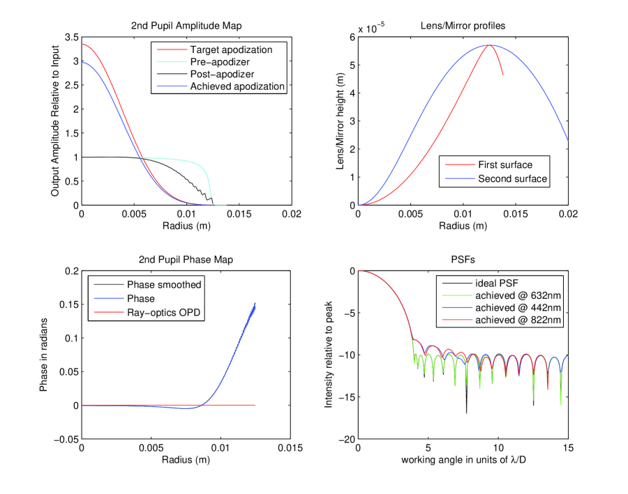
Figure 4: Analysis of an apodized pupil mapping system using the S-Huygens approximation with $z=15D$ and $n=1.5$. Upper-left plot shows in red the target high-contrast amplitude profile and in blue the amplitude profile computed using the S-Huygens approximation through the apodized pupil mapping system. The other two curves depict the pre- and post-apodizers. Upper-right plot shows the lens profiles, red for the first lens and blue for the second. The lens profiles $h$ and $\tilde{h}$ were computed using a $5,000$ point discretization. Lower-left plot shows in red the computed optical path length $Q_{0}(\tilde{r})$ and in blue the phase map computed using the S-Huygens propagation computed using a $5,000$ point discretization. Lower-right plot shows the PSF computed at three different wavelengths; the design value, $30\%$ above that value, and $30\%$ below it.

Figure 4 shows plots characterizing the performance of an apodized pupil mapping system analyzed using the techniques described in this section. The specifications for this system are as follows. The designed-for wavelength is $632.8$nm. The optical elements are assumed to be mirrors separated by $0.375$m. The system is an on-axis system and we therefore make the non-physical assumption that the mirrors don’t obstruct the beam. That is, the mirrors are invisible except when they are needed. The mirrors take as input a $0.025$m on-axis beam and produce a $0.025$m pupil-remapped exit beam. The second mirror is oversized by a factor of two; that is, its diameter is $0.050$m. The postapodizer ensures that only the central half contributes to the exit beam. The first mirror is also oversized appropriately as shown in the upper-right subplot of Figure 4. After the second mirror, the exit beam is brought to a focus. The focal length is $2.5$m. The lower-right subplot in Figure 4 shows the ideal PSF (in black) together with the achieved PSF at three wavelengths: at $70\%$ (green), $100\%$ (blue), and $130\%$ (red) of the design wavelength. At the design wavelength, the achieved PSF matches the ideal PSF almost exactly. Note that there is minor degradation at the other two wavelengths mostly at low spatial frequencies.

We end this section by pointing out that the S-Huygens approximation given by (15) is the basis for all subsequent analysis in this paper. It can be used to compute the propagation between every pair of consecutive components in apodized pupil mapping and concentric ring systems. It should be noted that the approximation does not reduce to the standard Fresnel or Fourier approximations even when considering such simple scenarios as free-space propagation of a plane wave or propagation from a pupil plane to an image plane. Even for these elementary situations, the S-Huygens approximation is superior to the usual textbook approximations.

3.2 Propagation of Azimuthal Harmonics

In this section, we assume that $E(r,\theta)=E(r)e^{in\theta}$ for some integer $n$. We refer to such a field as an $n$th-order azimuthal harmonic. We will show that an $n$th-order azimuthal harmonic will remain an $n$th-order azimuthal harmonic after propagating from the input plane to the output plane described in the previous section. Only the radial component $E(r)$ changes, which enables the reduction of the computation from 2D to 1D. Arbitrary fields can also be propagated, by decomposing them into azimuthal harmonics and propagating each azimuthal harmonic separately. Computation is thus greatly simplified even for arbitrary fields, especially for the case of fields which can be described by only a few azimuthal harmonics to a high precision, such as Zernike aberrations, which we consider in subsection 3.3. This improvement in computation efficiency is important, because a full 2D diffraction simulation of an apodized pupil mapping system with the precision of greater than $10^{10}$ typically overwhelms the memory of a mainstream computer. By reducing the computation from 2D to 1D, however, the entire apodized pupil mapping system can be simulated with negligible memory requirements and takes only minutes.

Theorem 1

Suppose that the input field in an optical system described by (15) is an $n$th-order azimuthal harmonic $E_{\mathrm{in}}(r,\theta)=E_{\mathrm{i}}(r)e^{in\theta}$ for some integer $n$. Then the output field is also an $n$th-order azimuthal harmonic $E_{\mathrm{out}}(\tilde{r},\tilde{\theta})=E_{\mathrm{o}}(\tilde{r})e^{in\tilde{\theta}}$ with radial part given by

$$E_{\mathrm{o}}(\tilde{r})=\frac{2\pi i^{n-1}A_{\mathrm{out}}(\tilde{r})}{\lambda Z}\int_{0}^{\infty}K(r,\tilde{r})E_{\mathrm{i}}(r)J_{n}\left(\frac{2\pi r\tilde{r}}{\lambda S(\tilde{r},r,0)}\right)\;A_{\mathrm{in}}(r)rdr.$$

Proof. We start by substituting the azimuthal harmonic form of $E_{\mathrm{in}}$ into (15) and regrouping factors to get

$$E_{\mathrm{out}}(\tilde{r},\tilde{\theta}) = \frac{A_{\mathrm{out}}(\tilde{r})}{\lambda iZ}\int_{0}^{\infty}K(r,\tilde{r})\int_{0}^{2\pi}e^{2\pi i\left(-\frac{\tilde{r}r\cos(\theta-\tilde{\theta})}{S(\tilde{r},r,0)}\right)/\lambda}E_{\mathrm{i}}(r)e^{in\theta}d\theta\;A_{\mathrm{in}}(r)rdr$$

$$= \frac{A_{\mathrm{out}}(\tilde{r})}{\lambda iZ}e^{in\tilde{\theta}}\int_{0}^{\infty}K(r,\tilde{r})E_{\mathrm{i}}(r)\int_{0}^{2\pi}e^{2\pi i\left(-\frac{\tilde{r}r\cos(\theta-\tilde{\theta})}{S(\tilde{r},r,0)}\right)/\lambda}e^{in(\theta-\tilde{\theta})}d\theta\;A_{\mathrm{in}}(r)rdr.$$

The result then follows from an explicit integration over the $\theta$ variable:

$$E_{\mathrm{out}}(\tilde{r},\tilde{\theta}) = \frac{2\pi i^{n-1}A_{\mathrm{out}}(\tilde{r})}{\lambda Z}e^{in\tilde{\theta}}\int_{0}^{\infty}K(r,\tilde{r})E_{\mathrm{i}}(r)J_{n}\left(\frac{2\pi r\tilde{r}}{\lambda S(\tilde{r},r,0)}\right)\;A_{\mathrm{in}}(r)rdr$$

$\Box$

3.3 Decomposition of Zernike Aberrations into Azimuthal Harmonics

The theorem shows that the full 2D propagation of azimuthal harmonics can be computed efficiently by evaluating a 1D integral. However, suppose that the input field is not an azimuthal harmonic, but something more familiar, such as a $(l,m)$-th Zernike aberration:

$$E_{\mathrm{in}}(r,\theta)=e^{i\epsilon Z_{l}^{m}(r/a)\cos(m\theta)},$$ (19)

where $\epsilon$ is a small number. ($\epsilon/2\pi$ and $\epsilon/\pi$ are the peak-to-valley phase variations across the aperture of radius $a$ for $m=0$ and $m\neq 0$, respectively.)

Recall that the definition of the $n$th-order Bessel function is

$$J_{n}(x)=\frac{1}{2\pi i^{n}}\int_{0}^{2\pi}e^{ix\cos\theta}e^{in\theta}d\theta.$$ (20)

From this definition we see that $i^{k}J_{n}(x)$ are simply the Fourier coefficients of $e^{ix\cos(\theta)}$. Hence, the Fourier series for the complex exponential is given simply by the so-called Jacobi-Anger expansion

$$e^{ix\cos\theta}=\sum_{k=-\infty}^{\infty}i^{k}J_{k}(x)e^{ik\theta}.$$ (21)

The Zernike aberration can be decomposed into azimuthal harmonics using the Jacobi-Anger expansion:

$$e^{i\epsilon Z_{l}^{m}(r/a)\cos(m\theta)} = \sum_{k=-\infty}^{\infty}i^{k}J_{k}(\epsilon Z_{l}^{m}(r/a))e^{ikm\theta}$$ (22)

$$= J_{0}(\epsilon Z_{l}^{m}(r/a))+\sum_{k=1}^{\infty}i^{k}J_{k}(\epsilon Z_{l}^{m}(r/a))e^{ikm\theta}$$ (23)

Note that

$$|J_{k}(x)|\approx\frac{1}{k!}\left(\frac{x}{2}\right)^{k}$$

for $0\leq x\ll 1$. Hence, if we assume that $\epsilon\sim 10^{-3}$, then the $k$’th term is of the order $10^{-3k}$. The field amplitude in the high-contrast region of the PSF will be dominated by the $k=1$ term and be on the order of $10^{-3}$. If we drop terms of $k=3$ and above, we are introducing an error on the order of $10^{-9}$ in amplitude. The error in intensity will be dominated by a cross-product of the $k=3$ and the $k=1$ term, or $10^{-12}$ across the dark region. So, in this case, Zernike aberrations can be more than adequately modeled using just 3 azimuthal harmonic terms. For $\epsilon\sim 10^{-2}$, the number of terms goes up to 5 for an error tolerance of $10^{-12}$. In practice, even this small number of terms was actually found to be overly conservative.

In order to compute the full 2D response for a given Zernike aberration, we simply decompose it into a few azimuthal harmonics, propagate them separately, and sum the results at the end. This method could also be applied to any arbitrary field.

4 Simulations

The entire 4-mirror apodized pupil mapping system can be modeled as the following sequence of 7 steps:

1. Propagate an input wavefront from the front (flat) surface of the first pupil mapping lens to the back (flat) surface of the second pupil mapping lens as described in Section 2.3.

2. Propagate forward a distance $f$.

3. Propagate through a positive lens with focal length $f$ to a focal plane $f$ units downstream.

4. Multiply by star occulter.

5. Propagate through free-space a distance $f$ then through a positive lens to recollimate the beam.

6. Propagate forward a distance $f$.

7. Propagate backwards through a pupil mapping system having the same parameters as the first one.

A similar analysis can be carried out for a concentric ring shaped pupil system, or even a pure apodization system, as follows:

1. Choose $A_{\mathrm{in}}$ to represent either the concentric ring binary mask or some other azimuthally symmetric apodization.

2. Choose $h$ as appropriate for a focusing lens and let $\tilde{h}\equiv 0$.

3. Propagate through this system a distance $f$ to the image plane.

4. Multiply by star occulter.

The theorem can be applied to every propagation step, so that an azimuthal harmonic will remain an azimuthal harmonic throughout the entire system. Hence, our computation strategy was to decompose the input field into azimuthal harmonics, propagate each one separately through the entire system by repeated applications of the theorem, and sum them at the very end.

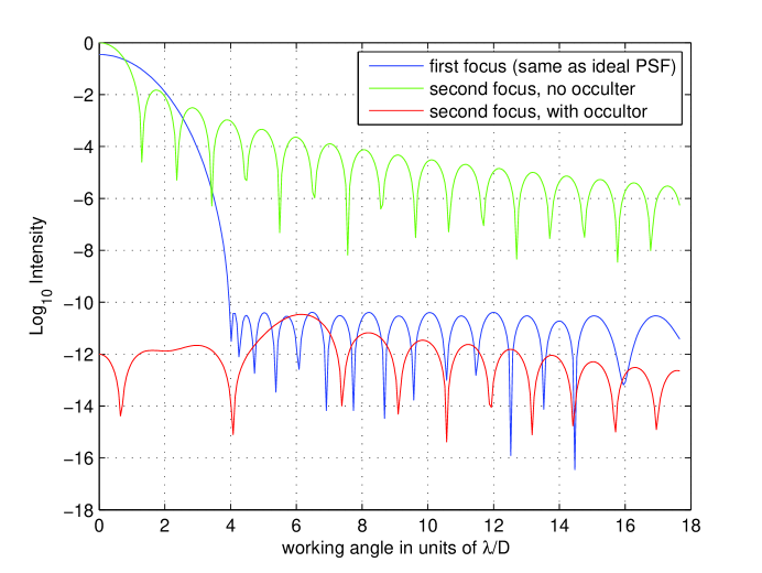
Figure 5: On-axis PSF at first focus (before occulter) and at second focus for cases of with and without occulter. Without the occulter, the second-focus PSF almost perfectly matches the usual Airy pattern. However, with the occulter, the second-focus on-axis PSF is suppressed by ten orders of magnitude.

Figure 5 shows a cross section plot of the PSF as it appears at first focus and second focus in our apodized pupil mapping system (the first focus plot is indistinguishable from the case of ideal apodization or concentric ring shaped pupils). There are two plots for second focus: one with the occulter in place and one without it. Note that without the occulter, the PSF matches almost perfectly the usual Airy pattern. With the occulter, the on-axis light is suppressed by ten orders of magnitude.

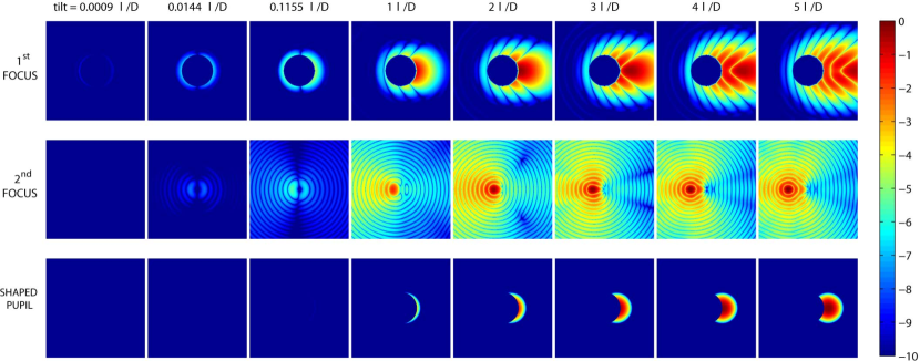
Figure 6: 2D pictures of planets for apodized pupil mapping and concentric rings. First row shows 2D intensity plots at first focus behind the occulter for planets at various angles relative to the on-axis star. Note that the system fails to form a clean image of the planets. Second row shows analogous plots at second focus. Note that the wavefront for the off-axis planet is mostly restored and the images begin to look like standard Airy patterns as the angle increases. Third row shows analogous plots for a concentric ring mask.

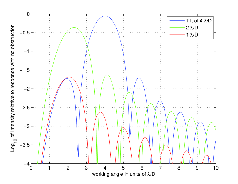
Figure 7: Cross-sectional plots from the second row plots in Figure 6. Note that for angles of $3\lambda/D$ and above, the restored PSF looks very much like an Airy pattern with very little energy attenuation. However, as the angle decreases, the pattern begins to distort and the throughput begins to diminish.

The electric field for a planet is just a slightly tilted and much fainter field than the field associated with the star. Hence, the methods presented here (specifically using the $(1,1)$-Zernike, i.e. tilt) can be used to generate planet images. Some such scenarios are shown in Figure 6. The first row shows how an off-axis source, i.e. planet, looks at the first focus. As discussed earlier, at this focal plane off-axis sources do not form good images. This is clearly evident in this figure. The second row shows the planet as it appears at the second image plane, which is downstream from the reversed pupil mapping system. In this case, the off-axis source is mostly restored and the images begin to look like standard Airy patterns as the angle increases from about $2\lambda/D$ outward. Figure 7 shows corresponding cross sectional plots for the apodized pupil mapping system at the second focus. The third row in Figure 6 shows how a planet would appear at a focal plane of a concentric ring shaped pupil system.

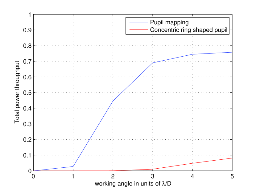
Figure 8: Off-axis source attenuation as a function of angle. Note that the $50\%$ point occurs at about $2.5\lambda/D$.

Figure 8 shows how the off-axis source is attenuated as a function of the angle from optical axis, for the case of our apodized pupil mapping system (at second focus) and the concentric ring coronagraph. For the case of apodized pupil mapping, the $50\%$ point occurs at about $2.5\lambda/D$.

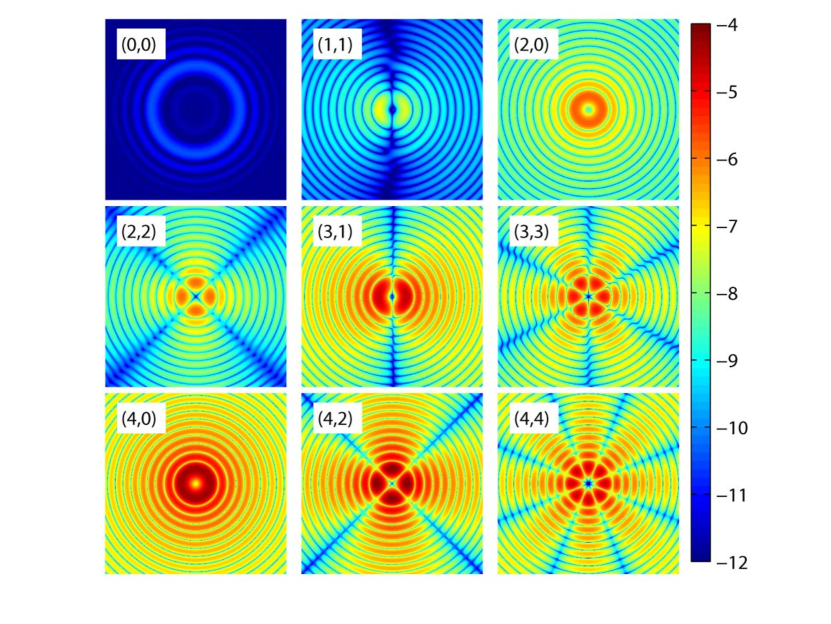
Figure 9: Apodized pupil mapping sensitivities to the first nine Zernike aberrations. In each case, the rms error is $1/100$th wave. The plots correspond to: Piston $(0,0)$, Tilt $(1,1)$, Defocus $(2,0)$, Astigmatism $(2,2)$ Coma $(3,1)$, Trefoil $(3,3)$, Spherical Aberration $(4,0)$, Astigmatism 2nd Order $(4,2)$, Tetrafoil $(4,4)$.

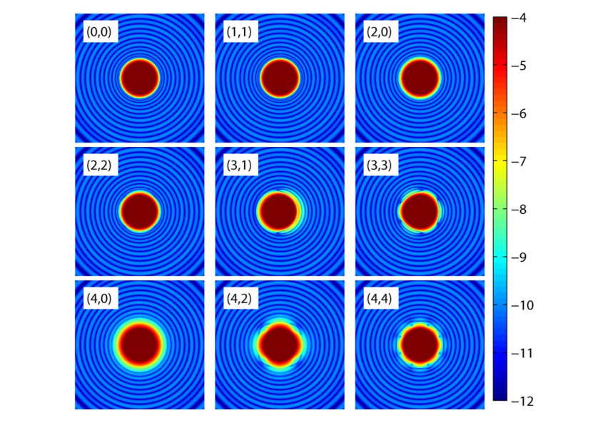
Figure 10: Concentric-ring mask sensitivities to the first nine Zernike aberrations.

Figures 9 and 10 show the distortions/leakage from an on-axis source in the presence of various Zernike aberrations, for apodized pupil mapping and the concentric ring shaped pupil systems, respectively. The Zernike aberrations are assumed to be $1/100$th wave rms.

Figure 11 shows the corresponding cross-section sensitivity plots for both the apodized pupil mapping system and the concentric ring shaped pupil system. From this plot it is easy to see both the tighter inner working angle of apodized pupil mapping systems as well as their increased sensitivity to wavefront errors. Finally, Figure 12 demonstrates contrast degradation measured at three angles, $2$, $4$, and $8\lambda/D$, as a function of severity of the Zernike wavefront error. The rms error is expressed in waves.

5 Conclusions

We have presented an efficient method for calculating the diffraction of aberrations through optical systems such as apodized pupil mapping and shaped pupil coronagraphs. We presented an example for both systems and computed their off-axis responses and aberration sensitivities. Figures 11 and 12 show that our particular apodized pupil mapping system is more sensitive to low order aberrations than the concentric ring masks. That is, contrast and IWA degrade more rapidly with increasing rms level of the aberrations. Thus, for a particular telescope, our pupil mapping system will achieve better throughput and inner working angle, but suffer greater aberration sensitivity.

We note that there is a spectrum of apodized pupil mapping systems, out of which we selected but one example. The two extremes, pure apodization and pure pupil mapping, both have serious drawbacks. On the one end, pure apodization loses almost an order of magnitude in throughput and suffers from an unpleasantly large IWA. At the other extreme, pure pupil mapping fails to achieve the required high contrast due to diffraction effects. There are several points along this spectrum that are superior to the end points. We have focused on just one such point, which is similar to the design suggested by Guyon et al. (2005). We leave it to future work to determine if this is the best design point. For example, clearly one can improve the aberration sensitivity by relaxing the inner working angle and throughput requirements. Such analysis is beyond the scope of this paper, but we have provided here the tools to analyze the sensitivity of these kinds of designs.

Acknowledgements. This research was partially performed for the Jet Propulsion Laboratory, California Institute of Technology, sponsored by the National Aeronautics and Space Administration as part of the TPF architecture studies and also under JPL subcontract number 1260535. The third author also received support from the ONR (N00014-05-1-0206).

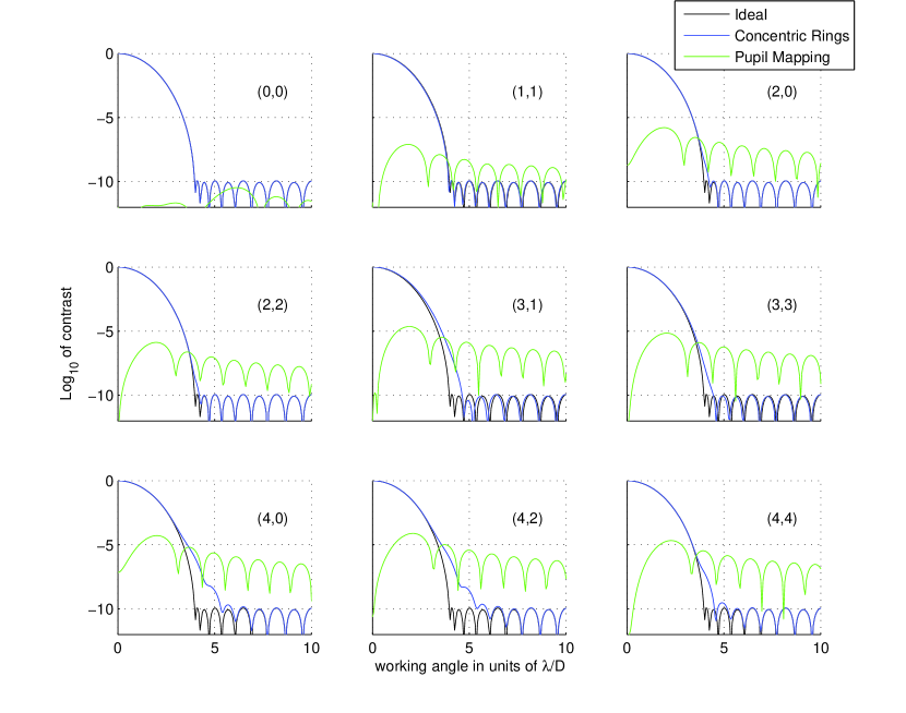
Figure 11: Radial profiles associated with the previous two Figures and overlayed one on the other. The green plots are for apodized pupil mapping whereas the blue plots are for the concentric ring mask.

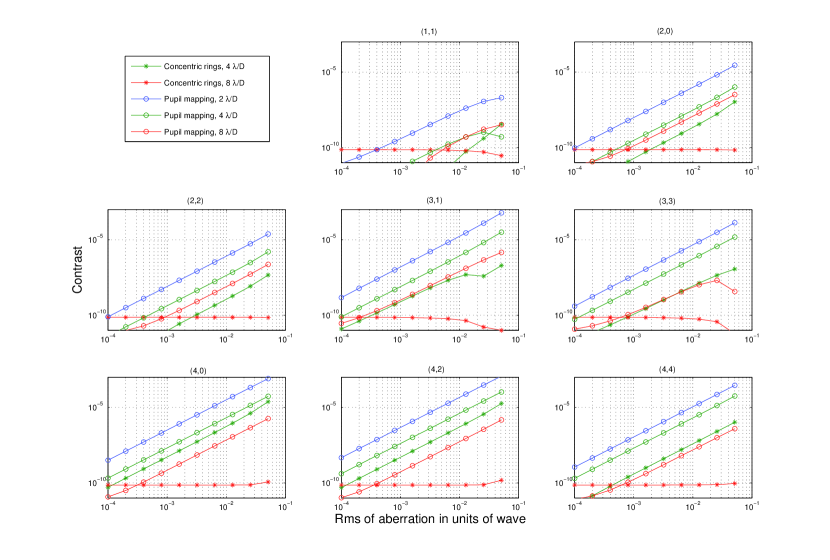
Figure 12: Contrast degradation measured at three angles, $2$, $4$, and $8\lambda/D$ as a function of severity of the Zernike wavefront error measured in waves.

References

- Born and Wolf (1999) M. Born and E. Wolf. Principles of Optics. Cambridge University Press, New York, NY, 7th edition, 1999.
- Carney and Gbur (1999) P.S. Carney and G. Gbur. Optimal apodizations for finite apertures. Journal of the Optical Society of America A, 16(7):1638–1640, 1999.
- Goncharov et al. (2002) A. Goncharov, M. Owner-Petersen, and D. Puryayev. Intrinsic apodization effect in a compact two-mirror system with a spherical primary mirror. Opt. Eng., 41(12):3111, 2002.
- Green et al. (2004) J.J. Green, S.B. Shaklan, R.J. Vanderbei, and N.J. Kasdin. The sensitivity of shaped pupil coronagraphs to optical aberrations. In Proceedings of SPIE Conference on Astronomical Telescopes and Instrumentation, 5487, pages 1358–1367, 2004.
- Guyon (2003) O. Guyon. Phase-induced amplitude apodization of telescope pupils for extrasolar terrerstrial planet imaging. Astronomy and Astrophysics, 404:379–387, 2003.
- Guyon et al. (2005) O. Guyon, E.A. Pluzhnik, R. Galicher, R. Martinache, S.T. Ridgway, and R.A. Woodruff. Exoplanets imaging with a phase-induced amplitude apodization coronagraph–i. principle. Astrophysical Journal, 622:744, 2005.
- Hoffnagle and Jefferson (2003) J.A. Hoffnagle and C.M. Jefferson. Beam shaping with a plano-aspheric lens pair. Opt. Eng., 42(11):3090–3099, 2003.
- Kasdin et al. (2003) N.J. Kasdin, R.J. Vanderbei, D.N. Spergel, and M.G. Littman. Extrasolar Planet Finding via Optimal Apodized and Shaped Pupil Coronagraphs. Astrophysical Journal, 582:1147–1161, 2003.
- Kuchner et al. (2004) M.J. Kuchner, J. Crepp, and J. Ge. Finding terrestrial planets using eighth-order image masks. Submitted to The Astrophysical Journal, 2004. (astro-ph/0411077).
- Pluzhnik et al. (2006) E.A. Pluzhnik, O. Guyon, S.T. Ridgway, R. Martinache, R.A. Woodruff, C. Blain, and R. Galicher. Exoplanets imaging with a phase-induced amplitude apodization coronagraph–iii. hybrid approach: Optical design and diffraction analysis. Submitted to The Astrophysical Journal, 2006. (astro-ph/0512421).
- Shao et al. (2004) M. Shao, B.M. Levine, E. Serabyn, J.K. Wallace, and D.T. Liu. Visible nulling coronagraph. In Proceedings of SPIE Conference on Astronomical Telescopes and Instrumentation, number 61 in 5487, 2004.
- Slepian (1965) D. Slepian. Analytic solution of two apodization problems. Journal of the Optical Society of America, 55(9):1110–1115, 1965.
- Traub and Vanderbei (2003) W.A. Traub and R.J. Vanderbei. Two-Mirror Apodization for High-Contrast Imaging. Astrophysical Journal, 599:695–701, 2003.
- Vanderbei et al. (2004) R. J. Vanderbei, N. J. Kasdin, and D. N. Spergel. Checkerboard-mask coronagraphs for high-contrast imaging. Astrophysical Journal, 615(1):555, 2004.
- Vanderbei (2006) R.J. Vanderbei. Diffraction analysis of 2-d pupil mapping for high-contrast imaging. Astrophysical Journal, 636:528, 2006.
- Vanderbei et al. (2003a) R.J. Vanderbei, D.N. Spergel, and N.J. Kasdin. Circularly Symmetric Apodization via Starshaped Masks. Astrophysical Journal, 599:686–694, 2003a.
- Vanderbei et al. (2003b) R.J. Vanderbei, D.N. Spergel, and N.J. Kasdin. Spiderweb Masks for High Contrast Imaging. Astrophysical Journal, 590:593–603, 2003b.