Synchrotron emission in small scale magnetic field as possible explanation for prompt emission spectra of Gamma-Ray bursts

Abstract

Synchrotron emission is believed to be a major radiation mechanism during gamma-ray bursts’ (GRBs) prompt emission phase. A significant drawback of this assumption is that the theoretical predicted spectrum, calculated within the framework of the “internal shocks” scenario using the standard assumption that the magnetic field maintains a steady value throughout the shocked region, leads to a slope $F_{\nu}\propto\nu^{-1/2}$ below $100\rm{\,keV}$, which is in contradiction to the much harder spectra observed. This is due to the electron cooling time being much shorter than the dynamical time. In order to overcome this problem, we propose here that the magnetic field created by the internal shocks decays on a length scale much shorter than the comoving width of the plasma. We show that under this assumption synchrotron radiation can reproduce the observed prompt emission spectra of the majority of the bursts. We calculate the required decay length of the magnetic field, and find it to be $\sim 10^{4}-10^{5}$ cm (equivalent to $10^{5}-10^{6}$ skin depths), much shorter than the characteristic comoving width of the plasma, $\sim 3\times 10^{9}$ cm. We implement our model to the case of GRB050820A, where a break at $\lesssim 4\rm{\,keV}$ was observed, and show that this break can be explained by synchrotron self absorption. We discuss the consequences of the small scale magnetic field scenario on current models of magnetic field generation in shock waves.

1. Introduction

A widely accepted interpretation of the non-thermal radiation observed during the prompt emission phase of gamma-ray bursts (GRBs) is that synchrotron emission is a leading radiation mechanism during this phase (Mészáros et al. , 1993; Mészáros & Rees, 1993a, b; Mészáros et al. , 1994; Katz, 1994; Rees & Mészáros, 1994; Tavani, 1996a). Indeed, early works found that the majority of bursts show spectral slopes in the $\sim 1-200\rm{\,keV}$ range of $\nu F_{\nu}\propto\nu^{\alpha}$, with $\alpha\simeq 4/3$ (Tavani, 1996a, b; Cohen et al. , 1997; Schaefer et al. , 1998; Frontera et al. , 2000), which is in accordance with the predictions of the optically thin synchrotron emission model, provided that the synchrotron cooling time of the radiating electrons is longer than the emission time. In addition, recent comprehensive analysis of the brightest BATSE bursts (Preece et al. , 2000; Kaneko et al. , 2006) found that the distribution of the low energy spectral slope peaks at $\alpha\simeq 1$, and a significant fraction of the bursts show spectral slope consistent with $\alpha\simeq 4/3$.

The idea that synchrotron emission is the leading radiation mechanism had gained further support by modeling the more detailed observations of the afterglow phase in GRBs, which are found to be in good agreement with this model prediction (Sari et al. , 1996; Mészáros & Rees, 1997; Waxman, 1997a, b; Sari et al. , 1998; Panaitescu & Mészáros, 1998; Wijers & Galama, 1999).

In the standard internal/external shock scenario of GRBs (the “fireball” model scenario; Rees & Mészáros, 1992, 1994; Sari & Piran, 1997), magnetic fields are generated by shock waves. Electrons are accelerated to high energies by the same shock waves, which thus provide the necessary conditions for synchrotron radiation. The mechanisms of energy transfer to the magnetic field and to accelerated electrons are not fully understood. It is therefore common to parametrize the energy densities in the magnetic field and in the energetic electrons as fractions $\epsilon_{B}$ and $\epsilon_{e}$ of the post shock thermal energy, where the values of $\epsilon_{e}$ and $\epsilon_{B}$ are inferred from observations. By modeling GRB afterglow emission data (Wijers & Galama, 1999; Freedman & Waxman, 2001; Panaitescu & Kumar, 2001, 2002), the parameters values are found to be at least few percents in most of the cases, and in some cases close to equipartition (Wijers & Galama, 1999; Frail et al. , 2000).

The fact that a significant fraction of the bursts show spectra that are too hard to account for in the optically thin synchrotron model (Crider et al. , 1997; Preece et al. , 1998, 2002; Ghirlanda et al. , 2003) had motivated works on alternative emission models. These include Synchrotron self Compton (SSC) scattering, first suggested by Liang (1997); Liang et al.  (1997), Compton drag (Lazzati et al. , 2000), upscattering of synchrotron self absorbed photons (Ghisellini & Celotti, 1999; Panaitescu & Mészáros, 2000; Kumar et al. , 2006), and Compton scattering of photospheric photons (Mészáros & Rees, 2000; Mészáros et al. , 2002; Pe’er et al. , 2005, 2006, and references therein). While in principle these models can reproduce a hard spectral slope, common requirements to all models involved inverse Compton scattering as a leading radiation mechanism is that at the emission radius the optical depth to scattering is high, and that $\epsilon_{B}/\epsilon_{e}\ll 1$. This last requirement, in turn, can lead to extensive radiation at very high ($\gg\rm{\,MeV}$) energies, thus to low radiative efficiency at the sub-MeV energy range (Derishev et al. , 2001). Additional drawback of SSC models is the wider spread in the peak energy distribution (compared to synchrotron model results for similar range of parameter dispersion), which might not be consistent with the data (e.g., Zhang & Mészáros, 2002). Therefore, these models put various constraints on the allowed parameter space region during the emission phase (e.g., Zhang & Mészáros, 2004; Pe’er & Waxman, 2004).

An argument raised against the synchrotron mechanism [Ghisellini et al.  (2000); see also discussion in Zhang & Mészáros (2004)] is that the inferred values of the free model parameters, in particular the strength of the comoving magnetic field during the prompt emission phase, $B^{\prime}\sim 10^{5}-10^{6}$ G, implies that the radiating electrons are synchrotron cooled much faster than the dynamical time. This, in turn, leads to a spectrum with slope $\nu F_{\nu}\propto\nu^{1/2}$ below $\sim 100\rm{\,keV}$, which is in conflict to the much harder spectra observed in this energy range. In order to overcome this problem, it was suggested that the energy distribution of radiating electrons has a smooth cutoff, and that the pitch angles of these electrons are anisotropically distributed (Lloyd & Petrosian, 2000; Lloyd-Ronning & Petrosian, 2002).

A crucial underlying assumption in this analysis, is that electrons radiate on a length scale comparable to the entire comoving width of the shocked plasma. For plausible assumptions about the number density and characteristic Lorentz factors in GRBs, this assumption can only hold if the magnetic field maintains approximately constant value on a scale of $\approx 10^{9}$ skin depth (Piran, 2005).

Generation of magnetic field in strong, relativistic shock waves is still poorly understood. Two stream instability of flow past shock waves can, in principle generate strong magnetic field (Medvedev & Loeb, 1999). However, state of the art numerical models (Silva et al. , 2003; Frederiksen et al. , 2004; Nishikawa et al. , 2005) can only trace the evolution of this field on a characteristic scale of few tens of skin depths at most, due to the huge numerical effort involved. The evolution of the magnetic field on larger scale therefore still remains an open question. While some models predict that the magnetic field saturates at a value close to equipartition (e.g., Jaroschek et al. , 2004), several authors find much weaker magnetic field (Wiersma & Achterberg, 2004), or argued that the created magnetic field quickly decays by phase-space mixing (Gruzinov, 2001).

Motivated by these uncertainties on the length scale of the magnetic field, Rossi & Rees (2003) suggested a model for GRB afterglow emission, in which the magnetic field decays on a length scale shorter than the shocked region scale. In that work, however, the decay length of the magnetic field was not specified.

In this paper we show that by assuming that the magnetic field decays on a length scale shorter than the comoving scale, the observed prompt emission spectra of many GRBs can be reproduced. Thereby, this assumption allows to overcome the “fast cooling time” problem inferred by Ghisellini et al.  (2000). We calculate in section §2 the values of the free model parameters that can account for the GRBs prompt emission spectra. We show that the decay length of the magnetic field that is consistent with the observed spectra is $\sim 10^{4}-10^{5}$ cm, which is $\approx 10^{5.5}$ skin depths. We then implement our model in section §3 to the specific case of GRB050820A, where a low energy break at $\sim 4\rm{\,keV}$ was observed. We summarize our results and discuss the implications of our model in view of current models of magnetic field generation in relativistic shock waves in section §4.

2. Theory of small magnetic field length scale: constraints on model parameters set by observations

We adopt the framework of the internal shock scenario and assume that variability in the Lorentz factor $\Gamma$ of the relativistic wind emitted by the GRB progenitor leads to the formation of shock waves within the expanding wind at radii much larger than the underlying source size (see, e.g., Zhang & Mészáros, 2002). We assume that these shock waves, produced at characteristic radius $r$ from the progenitor, are the source of the magnetic field. We introduce a new length scale $\Delta r^{\prime}_{B}$, which is the comoving length scale characterizing the decay of the magnetic field. This decay length is much shorter than the comoving width of the plasma $\Delta r^{\prime}\simeq r/\Gamma$. We derive in this section the constraints on the model parameters as inferred from observations.

The radiating electrons are accelerated by the shock waves to a power law distribution with power law index $p$ above some characteristic energy $\gamma_{\min}m_{e}c^{2}$. Synchrotron radiation by these electrons is the main emission mechanism, therefore the break energy observed in many bursts at $\varepsilon_{m}^{ob.}\gtrsim 100\rm{\,keV}$ is attributed to synchrotron radiation from electrons at $\gamma_{\min}$. Denoting by $\gamma_{c}$ the Lorentz factor of electrons that cool on a time scale equal to the dynamical timescale, and by $\varepsilon_{c}^{ob.}$ the characteristic observed energy of photons emitted by synchrotron radiation from these electrons, the requirement that the spectral slope $\nu F_{\nu}\propto\nu^{\alpha}$ has a characteristic spectral index $\alpha\simeq 4/3$ below $\sim 100\rm{\,keV}$ leads to $\varepsilon_{c}^{ob.}\gtrsim 100\rm{\,keV}$. The value of $\varepsilon_{c}^{ob.}$ can not be much greater than $100\rm{\,keV}$, in order to ensure high radiative efficiency (see discussion in §4 below).

The requirement that the spectral slope is not harder than $4/3$, as is the case in a significant fraction of the bursts, implies that in these bursts inverse Compton scattering and thermal emission component do not play a significant role in producing the spectra below $100\rm{\,keV}$. These conditions can be translated to the demand that the emission radius $r$ is larger than the photospheric radius, $r_{ph}$. Additional two constraints are that the observed flux $\nu F_{\nu}$ and the synchrotron self absorption energy $\varepsilon_{ssa}^{ob.}$, which produces a low energy break, are consistent with observations.

The observational constraints can therefore be written as a set of equations in the form:

$$\begin{array}[]{llll}(a)&\varepsilon_{m}^{ob.}&\gtrsim 100&\rm{\,keV},\\ (b)&\varepsilon_{c}^{ob.}&\gtrsim 100&\rm{\,keV},\\ (c)&r&\gtrsim r_{ph}&,\\ (d)&\nu F_{\nu}^{ob.}&\simeq 10^{-7}&{\rm\,erg\,s^{-1}\,cm^{-2}},\\ (e)&\varepsilon_{ssa}^{ob.}&\lesssim 1&\rm{\,keV},\end{array}$$

We now apply the set of equations (2) describing the constraints set by observations to constraints on the uncertain values of the free model parameters.

Assuming variability in the Lorentz factor $\Delta\Gamma/\Gamma\sim 1$ on timescale $\Delta t$ of the expanding relativistic wind, shocks develop at radius $r\simeq\Gamma^{2}c\Delta t$. Due to Lorentz contraction, the comoving width of a plasma shell is $\Delta r^{\prime}\simeq r/\Gamma$. We use the standard fireball model assumption, in which the burst explosion energy is initially converted to kinetic energy. For isotropically equivalent central engine luminosity $L$ which is time independent over a period $\Delta t$, the isotropically equivalent number of protons ejected from the progenitor during this period is $N_{p}\approx L\Delta t/\Gamma m_{p}c^{2}$. Therefore, the comoving number density of protons in the shock heated plasma is given by

$$n_{p}^{\prime}(r)\approx{\zeta L\over 4\pi r^{2}\Gamma^{2}cm_{p}c^{2}}=1.8\times 10^{13}\,L_{52}\,r_{13}^{-2}\,\Gamma_{2}^{-2}\,\zeta_{0}\,{\rm cm^{-3}},$$ (1)

where $\zeta$ is the compression ratio ($\zeta\simeq 7$ for strong shocks) and the convention $Q=10^{x}Q_{x}$ is adopted in CGS units. Assuming that the proton internal energy (associated with the random motion) in the shocked plasma is $\theta_{p}m_{p}c^{2}$, the comoving internal energy density is $u^{\prime}=n_{p}^{\prime}\theta_{p}m_{p}c^{2}$. The value of $\theta_{p}$ is not expected to be much larger than a few at most for mildly relativistic (in the comoving frame) shock waves. The magnetic field carries a fraction $\epsilon_{B}$ of the internal energy density, thus the comoving magnetic field strength is given by

$$\begin{array}[]{lll}B^{\prime}&=&\sqrt{8\pi\epsilon_{B}u^{\prime}}\\ &=&4.6\times 10^{5}\,L_{52}^{1/2}\,r_{13}^{-1}\,\Gamma_{2}^{-1}\,\epsilon_{B,-0.5}^{1/2}\,\theta_{p,0}^{1/2}\,\zeta_{0}^{1/2}{\rm\,G}.\end{array}$$

We assume that a fraction $\epsilon_{pl}\leq 1$ of the electron population is accelerated by the shock waves to a power law energy distribution with power law index $p$ above $\gamma_{\min}$ (and below $\gamma_{\max}$). Assuming that a fraction $\epsilon_{e}$ of the post-shock thermal energy is carried by these electrons, the minimum Lorentz factor of the energetic electrons is given by

$$\begin{array}[]{lll}\gamma_{\min}&=&{\epsilon_{e}\theta_{p}\over\epsilon_{pl}}\left({m_{p}\over m_{e}}\right){1-(\gamma_{\min}/\gamma_{\max})\over\log{\left({\gamma_{\max}\over\gamma_{\min}}\right)}}\times\Psi(p)\\ &=&86\,\epsilon_{e,-0.5}\,\epsilon_{pl,0}^{-1}\,\theta_{p,0}\,\Psi(p),\end{array}$$

where characteristic value $\log(\gamma_{\max}/\gamma_{\min})\simeq 7$ was used. The function $\Psi(p)$ determines the dependence of the value of $\gamma_{\min}$ on the power law index $p$ of the accelerated electrons, and is normalized to $\Psi(p=2)=1$. A full calculation of this function for various values of the power law index $p$ is given in appendix A.1. Using equations 2 and 2, the break in the spectrum from burst at redshift $z$ is observed at

$$\begin{array}[]{lll}\varepsilon_{m}^{ob.}&=&\left({1\over 1+z}\right){3\over 2}\hbar\Gamma{qB^{\prime}\gamma_{\min}^{2}\over m_{e}c}\\ &=&{5.9\over 1+z}\,L_{52}^{1/2}\,r_{13}^{-1}\,\epsilon_{e,-0.5}^{2}\,\epsilon_{pl,0}^{-2}\,\epsilon_{B,-0.5}^{1/2}\\ &&\times\theta_{p,0}^{5/2}\,\zeta_{0}^{1/2}\,\Psi^{2}(p)\rm{\,keV}.\end{array}$$

Electrons in the shocked region propagate at velocity close to the speed of light. Therefore, electrons cross the magnetized area in a comoving time $\approx\Delta r^{\prime}_{B}/c$. Since this is the available time for electrons to radiate, equating the synchrotron cooling time and the crossing time of this area gives the cooling break of the electrons energy distribution, which occurs at Lorentz factor $\gamma_{c}=(9m_{e}^{3}c^{6})/(4q^{4}B^{\prime 2}\Delta r^{\prime}_{B})$. Photons emitted by electrons at $\gamma_{c}$ are observed at energy

$$\varepsilon_{c}^{ob.}={97\over 1+z}\,L_{52}^{-3/2}\,r_{13}^{3}\,\Gamma_{2}^{4}\,\epsilon_{B,-0.5}^{-3/2}\,\Delta{r^{\prime}}_{B,7}^{-2}\,\theta_{p,0}^{-3/2}\,\zeta_{0}^{-3/2}\rm{\,eV}.$$ (2)

The number of radiating electrons is calculated by integrating the number density of energetic electrons inside the emitting region, $N_{e}(r)=4\pi\int_{r}^{r+\Delta r_{B}}r^{2}n(r)dr\simeq(\zeta\epsilon_{pl}L/\Gamma m_{p}c^{3})(\Delta r^{\prime}_{B}/\Gamma)$. Here, $\Delta r_{B}=\Delta r^{\prime}_{B}/\Gamma$ and $n(r)=\Gamma\epsilon_{pl}n^{\prime}_{p}(r)$ are the (observer frame) width and number density of radiating electrons inside this region .

By requirement, $\gamma_{c}\geq\gamma_{\min}$, therefore in calculating the observed flux, one can approximate the photon energy to be close to $\varepsilon_{m}^{ob.}$. The (frequency integrated) power emitted by electrons with Lorentz factor $\gamma_{\min}$ is $P(\gamma_{\min})=(4q^{4}B^{\prime 2}\gamma_{\min}^{2})/(9m_{e}^{2}c^{3})$, therefore the observed flux is

$$\begin{array}[]{lcl}\nu F_{\nu}^{ob.}&=&{P(\gamma_{\min})N_{e}(r)\over 4\pi d_{L}^{2}}\times\Gamma^{2}\\ &=&2.9\times 10^{-7}\,L_{52}^{2}\,r_{13}^{-2}\,\epsilon_{e,-0.5}^{2}\,\epsilon_{pl,0}^{-1}\,\epsilon_{B,-0.5}\\ &&\times\Delta{r^{\prime}}_{B,7}\,\Gamma_{2}^{-2}\rm{\,d_{L,28.5}^{-2}}\,\theta_{p,0}^{3}\,\zeta_{0}^{2}\,\Psi^{2}(p)\,\rm{\,erg\,cm^{-2}\,s^{-1}},\end{array}$$

where $d_{L}=10^{28.5}d_{L,28.5}\rm{\,cm}$ is the luminosity distance, and a factor $\Gamma^{2}$ is introduced to transform the result from the comoving frame to the observer frame.

The optical depth is given by $\tau(r)=n^{\prime}_{p}(r)\Delta r^{\prime}\sigma_{T}$, where the comoving width $\Delta r^{\prime}$ and not the comoving radiating width $\Delta r^{\prime}_{B}$ appears in the equation since electrons scatter photons outside the radiating region as well. The photospheric radius is thus given by

$$\begin{array}[]{lll}r_{ph}=r(\tau(r)=1)&=&{\zeta L\sigma_{T}\over 4\pi\Gamma^{3}m_{p}c^{3}}\\ &=&1.2\times 10^{13}\,L_{52}\,\Gamma_{2}^{-3}\,\zeta_{0}\,\rm{\,cm}.\end{array}$$

The observed synchrotron self absorption energy break is calculated using standard formula (e.g., Rybicki & Lightman, 1979)

$$\begin{array}[]{lll}\varepsilon_{ssa}^{ob.}&=&{31\over 1+z}\,L_{52}^{4/5}\,r_{13}^{-8/5}\,\Delta{r^{\prime}}_{B,7}^{3/5}\,\Gamma_{2}^{-3/5}\,\epsilon_{e,-0.5}^{-1}\,\epsilon_{pl,0}^{8/5}\,\epsilon_{B,-0.5}^{1/5}\\ &&\times\theta_{p,0}^{-4/5}\,\zeta_{0}^{4/5}\chi(p)\,\rm{\,eV},\end{array}$$

where $\chi(p)$ is a function of the power law index $p$ of the accelerated electrons, which is normalized to $\chi(p=2)=1$. We present in appendix A.2 a full derivation of this function, and show that its value strongly depends on the uncertain value of the power law index $p$ of the accelerated electrons.

While the first four constraints in equation 2 (a-d) are common to the majority of bursts, observation of a low energy break, which may be attributed to synchrotron self absorption frequency is controversial. We therefore treat the last constraint in equation 2 separately in section §3.

The constraints set by observations in equation 2 (a-d) can be written with the use of equations (2)-(2) in the form

$$\begin{array}[]{llcr}(a)&\left({5.9\over 1+z}\right)\,L_{52}^{1/2}\,r_{13}^{-1}\,\epsilon_{e,-0.5}^{2}\,\epsilon_{pl,0}^{-2}\,\epsilon_{B,-0.5}^{1/2}\,\theta_{p,0}^{5/2}\,\zeta_{0}^{1/2}\,\Psi^{2}(p)\\ &\qquad\qquad\qquad\;\,=100\,\alpha_{1},\\ (b)&\left({0.097\over 1+z}\right)\,L_{52}^{-3/2}\,r_{13}^{3}\,\Delta{r^{\prime}}_{B,7}^{-2}\,\Gamma_{2}^{4}\,\epsilon_{B,-0.5}^{-3/2}\,\theta_{p,0}^{-3/2}\,\zeta_{0}^{-3/2}\\ &\qquad\qquad\qquad\;\,=100\,\alpha_{2},\\ (c)&r_{13}\qquad\qquad\;\;\;=1.2\,L_{52}\,\Gamma_{2}^{-3}\,\zeta_{0}\,\alpha_{3},\\ (d)&2.9\,L_{52}^{2}\,r_{13}^{-2}\,\Delta{r^{\prime}}_{B,7}\,\Gamma_{2}^{-2}\,\epsilon_{e,-0.5}^{2}\,\epsilon_{pl,0}^{-1}\,\epsilon_{B,-0.5}\,\rm{\,d_{L,28.5}^{-2}}\\ &\times\theta_{p,0}^{3}\,\zeta_{0}^{2}\,\Psi^{2}(p)=1\,\alpha_{4},\\ \end{array}$$

where the free parameters $\alpha_{1}-\alpha_{4}$ are introduced in order to replace the inequalities in equation 2 by equalities, thereby account for the variety of GRB data.

In order to derive constraints on the values of the free model parameters from the set of equations 2 (a-d), we note that the parameters $\epsilon_{e}$ and $\epsilon_{B}$ are constrained from above by a maximum allowed value of equipartition ($\epsilon_{e,-0.5},\epsilon_{B,-0.5}\leq 1$). The parameter $\epsilon_{pl}$ also has an upper limit, $\epsilon_{pl}\leq 1$. Furthermore, the values of $\theta_{p}$, $\zeta$ and $\Psi(p)$ (for $p\geq 2$) can only be larger or equal to unity. In contrast to these constraints, there are no further intrinsic constraints on the values of the isotropic equivalent luminosity $L$, the emission radius $r$, the fluid Lorentz factor $\Gamma$ and the comoving decaying length of the magnetic field $\Delta r^{\prime}_{B}$. We therefore solve the set of equations 2 (a-d) to find the values of $L$, $r$, $\Gamma$ and $\Delta r^{\prime}_{B}$, and obtain

$$\begin{array}[]{lcll}L_{52}&=&2.7\;\;d_{L,28.5}^{2}\,\epsilon_{e,-0.5}^{-1}\,\theta_{p,0}^{-1}\,\zeta_{0}^{-1}\,\Psi^{-1}(p)\\ &&\times\alpha_{1}^{-1/2}\,\alpha_{2}^{1/2}\,\alpha_{4},\\ r_{13}&=&0.1\,(1+z)^{-1}\;\;d_{L,28.5}\,\epsilon_{e,-0.5}^{3/2}\,\epsilon_{pl,0}^{-2}\,\epsilon_{B,-0.5}^{1/2}\\ &&\times\theta_{p,0}^{2}\,\Psi^{3/2}(p)\,\alpha_{1}^{-5/4}\,\alpha_{2}^{1/4}\,\alpha_{4}^{1/2},\\ \Delta{r^{\prime}}_{B,7}&=&4.6\times 10^{-3}\,(1+z)^{-4/3}\;\;d_{L,28.5}^{2/3}\,\epsilon_{e,-0.5}^{4/3}\,\epsilon_{pl,0}^{-5/3}\\ &&\times\epsilon_{B,-0.5}^{-1/3}\,\theta_{p,0}\,\Psi^{4/3}(p)\,\alpha_{1}^{-1}\,\alpha_{2}^{-1/3}\,\alpha_{3}^{2/3}\,\alpha_{4}^{1/3},\\ \Gamma_{2}&=&3.2\,(1+z)^{1/3}\;\;d_{L,28.5}^{1/3}\,\epsilon_{e,-0.5}^{-5/6}\,\epsilon_{pl,0}^{2/3}\,\epsilon_{B,-0.5}^{-1/6}\\ &&\times\theta_{p,0}^{-1}\,\Psi^{-5/6}(p)\,\alpha_{1}^{1/4}\,\alpha_{2}^{1/12}\,\alpha_{3}^{1/3}\,\alpha_{4}^{1/6}.\end{array}$$

The values of the free model parameters derived in equation 2 indicate that the prompt emission spectra of the majority of the bursts can be explained in the framework of the model suggested here. For values of $\epsilon_{e}$ and $\epsilon_{B}$ not far below equipartition and $\epsilon_{pl}$ close to unity, these results imply that the emission radius should be $r\lesssim 10^{12}$ cm, and that the magnetic field decays on a comoving scale $\Delta r^{\prime}_{B}\sim 10^{4.5}$ cm. If only $\approx 10\%$ of the electrons are accelerated in the shock waves, $\epsilon_{pl}=0.1$, then the emission radius is significantly higher, $r\simeq 10^{14}$ cm, and the magnetic field decays after $\Delta r^{\prime}_{B}\sim 10^{6.5}$ cm. Interestingly, the derived values of the isotropically equivalent luminosity and the characteristic fluid Lorentz factor are not different than their derived values in the standard internal shock scenario. We further discuss the implications of these results in §4.

3. Possibility of a low energy break: The case of GRB050820A

The results obtained in the previous section in equation 2, may be applicable to many GRBs that show spectral slope $\nu F_{\nu}\propto\nu^{4/3}$ below $\sim 100\rm{\,keV}$. For the majority of GRBs observations during the prompt emission phase are available only above few $\rm{\,keV}$ (BATSE, Beppo-SAX or SWIFT BAT-XRT energy range). In most cases, observations do not indicate an additional low-energy break in the spectrum that might be attributed to synchrotron self absorption. On the contrary, in some cases (e.g., GRB060124; Romano et al. , 2006) interpolation of data taken in the UV band supports the lack of an additional spectral break above $\sim 1\rm{\,eV}$.

Even though uncommon to many GRBs, an additional, second low energy break may have been observed in some bursts. In at least one case - GRB050820A (Page et al. , 2005), there are indications for a low energy break at $\lesssim 4\rm{\,keV}$ observed during a gamma-ray/X-ray giant flare that occurred 218 seconds after the burst trigger, and lasted 34 seconds (Osborne, 2006). This low energy break may be attributed to synchrotron self absorption.

In order to account for these results in the framework of the model presented here, we insert the values of the four parameters $L$, $r$, $\Delta r^{\prime}_{B}$ and $\Gamma$ as inferred from the observational constraints in equation 2, to the equation describing the observed self absorption frequency (equation 2). This insertion results in

$$\begin{array}[]{lll}\varepsilon_{ssa}^{ob.}&=&56\,(1+z)^{-2/5}\,d_{L,28.5}^{1/5}\,\epsilon_{e,-0.5}^{-29/10}\,\epsilon_{pl,0}^{17/5}\,\epsilon_{B,-0.5}^{-7/10}\\ &&\times\theta_{p,0}^{-18/5}\,\tilde{\chi}(p)\,\alpha_{1}^{17/20}\,\alpha_{2}^{-1/4}\,\alpha_{3}^{1/5}\,\alpha_{4}^{1/10}\,\rm{\,eV},\end{array}$$

where $\tilde{\chi}(p)$ gives the dependence of $\varepsilon_{ssa}^{ob.}$ on the electrons power law index $p$, and is normalized to $\tilde{\chi}(p=2)=1$. We present in appendix A.2 a full derivation of this function, and show there that for values of $p$ in the range $2\leq p\leq 2.4$, this function varies by a factor less than 4. We can thus conclude that within the framework of the model suggested here, the self absorption energy is not very sensitive to the uncertain value of the power law index $p$ of the accelerated electrons.

While the the self absorption break calculated in equation 3 is clearly lower than the value of the break energy observed in GRB050820A, this equation indicates a very strong dependence of the break energy on the uncertain values of the parameters $\epsilon_{e}$, $\epsilon_{pl}$ and $\theta_{p}$. The equipartition value of $\epsilon_{e}$ used in equation 3 is an upper limit. If the value is $\epsilon_{e}\approx 0.1$, then the self absorption break is observed at $\sim 2\rm{\,keV}$. Similarly, for $\epsilon_{pl}\simeq 0.3$ or $\theta_{p}\approx 3$ , the self absorption break occurs at $\sim 1\rm{\,eV}$. Using the results of equation 2 we find that the values of the four other parameters $L$, $r$, $\Gamma$ and $\Delta r^{\prime}_{B}$ are much less sensitive to the uncertainties in $\epsilon_{e}$, $\epsilon_{pl}$ or $\theta_{p}$.

The parameters $\epsilon_{e}$, $\epsilon_{pl}$ and $\theta_{p}$ parametrize the post shock energy transfer to the electrons, the fraction of the electrons population accelerated by the shock waves, and the normalized mean random energy gained by proton population. All these physical quantities depend on the microphysics of energy transfer and particle acceleration in shock waves, both of which are not fully understood. We cannot therefore, from a theoretical point of view, rule out the possibility that the values of $\epsilon_{e}$, $\epsilon_{pl}$ and $\theta_{p}$ are sensitive to the plasma conditions at the shock forming region. Equation 3 combined with measurement (or constraint) on the self absorption frequency, can be used to constrain the uncertain values of these parameters.

4. Summary and discussion

In this work we have presented a model in which the magnetic field produced by internal shock waves in GRBs decays on a short length scale. Using this assumption, we showed that the prompt emission spectra of the majority of GRBs can be explained as due to synchrotron radiation from shock accelerated electrons. We found that the required (comoving) decay length of the magnetic field is $\sim 10^{4.5}$ cm, and that the radiation is produced at $\sim 10^{12}$ cm from the progenitor (eq. 2). These parameter values were found to be relatively sensitive to the fraction of electrons population accelerated by the shock waves $\epsilon_{pl}$, and can therefore be higher. We showed in §3 that the observed synchrotron self absorption energy is very sensitive to the uncertain values of the post shock thermal energy fraction carried by the electrons, to the mean proton energy $\theta_{p}$ and to the value of $\epsilon_{pl}$, thereby argued that the energy of a low energy break is expected to vary between different bursts.

A major result of this work is the characteristic decay length of the magnetic field deduced from observations, $\sim 10^{4.5}$ cm. This value is significantly shorter than the standard assumption used so far, that the magnetic field strength is approximately constant throughout the comoving plasma width, $\approx 10^{10}-10^{11}$ cm. Still, the electron crossing time of the magnetized region is long enough to allow electrons acceleration to high energies. Equating the electron acceleration time, $t_{acc}\simeq\gamma m_{e}c^{2}/(cqB^{\prime})$ and the electron crossing time, $\Delta r^{\prime}_{B}/c$, gives an upper limit on the electron Lorentz factor, $\gamma_{\max,1}=(\Delta r^{\prime}_{B}qB^{\prime})/(m_{e}c^{2})\simeq 2\times 10^{7}\,\Delta r^{\prime}_{B,4.5}B^{\prime}_{6}$, where $B^{\prime}=10^{6}B^{\prime}_{6}$ G. This value is larger than the maximum electron Lorentz factor obtained by equating the acceleration time and the synchrotron cooling time, $\gamma_{\max,2}=(3/2)(m_{e}c^{2})/(q^{3}B^{\prime})^{1/2}\simeq 10^{5}{B^{\prime}_{6}}^{-1/2}$. We thus conclude that within the magnetized region, for $\epsilon_{B}\gtrsim 10^{-3}$ an upper limit on the accelerated electron energy is set by the synchrotron cooling time, and not by the physical size of this region.

The parameters $\alpha_{1}-\alpha_{4}$ introduced in equations 2, 2 account for the difference between the variety of GRB data and the characteristic values considered in the analytical analysis. As a concrete example, cooling energy $\epsilon_{c}^{ob.}$ larger than $100\rm{\,keV}$ is accounted for by considering $\alpha_{2}>1$, which implies through equation 2 that high isotropic equivalent luminosity is required in order to account for an observed flux $\simeq 10^{-7}{\rm\,erg\,s^{-1}\,cm^{-2}}$. This result is understood as due to the low radiative efficiency in the case $\epsilon_{c}^{ob.}\gg\epsilon_{m}^{ob.}$.

The ratio found here between the decay length of the magnetic field and the comoving shell thickness,

$$\begin{array}[]{lll}{\Delta{r^{\prime}}_{B}\over(r/\Gamma)}&=&1.5\times 10^{-5}\,\epsilon_{e,-0.5}^{-1}\,\epsilon_{pl,0}\,\epsilon_{B,-0.5}^{-1}\,\theta_{p,0}^{-2}\,\Psi^{-1}(p)\\ &&\times\alpha_{1}^{1/2}\,\alpha_{2}^{-1/2}\,\alpha_{3},\end{array}$$

is based on fitting the GRB prompt emission spectra. In earlier work, based on modeling afterglow emission (Rossi & Rees, 2003), this value was thought to be too low, due to the high ambient medium density it implies during the afterglow emission phase. However, in the work by Rossi & Rees (2003) detailed modeling of afterglow data was not performed, due to lack of available data. Moreover, the well established connection between long GRBs and core collapse of massive stars (e.g., Pe’er & Wijers, 2006, and references therein) indicates that indeed the ambient medium density may be higher than previously thought.

The values of the parameters found in equation 2 imply that the comoving number density of the shocked plasma (equation 1) is

$$\begin{array}[]{lll}n_{p}^{\prime}&=&5.0\times 10^{14}\,(1+z)^{4/3}\,d_{L,28.5}^{-2/3}\,\epsilon_{e,-0.5}^{-7/3}\,\epsilon_{pl,0}^{8/3}\,\epsilon_{B,-0.5}^{-2/3}\\ &&\times\theta_{p,0}^{-3}\,\Psi^{-7/3}(p)\,\alpha_{1}^{3/2}\,\alpha_{2}^{-1/6}\,\alpha_{3}^{-2/3}\,\alpha_{4}^{-1/3}\,{\rm\,cm^{-3}}.\end{array}$$

For this value of the comoving number density, the plasma skin depth is given by

$$\begin{array}[]{lll}\lambda\simeq{c\gamma_{\min}^{1/2}\over\omega_{pe}}&=&0.2\,(1+z)^{-2/3}\,d_{L,28.5}^{1/3}\,\epsilon_{e,-0.5}^{5/3}\,\epsilon_{pl,0}^{-11/6}\,\epsilon_{B,-0.5}^{1/3}\\ &&\times\theta_{p,0}^{2}\,\Psi^{5/3}(p)\,\alpha_{1}^{-3/4}\,\alpha_{2}^{1/12}\,\alpha_{3}^{1/3}\,\alpha_{4}^{1/6}\,{\rm\,cm},\end{array}$$

where $\omega_{pe}=(4\pi q^{2}n_{p}^{\prime}/m_{e})^{1/2}$ is the plasma frequency. This value of the skin depth implies that the magnetic field decays on a characteristic length scale

$$\begin{array}[]{lll}{\Delta r^{\prime}_{B}\over\lambda}&=&2\times 10^{5}\,(1+z)^{-2/3}\,d_{L,28.5}^{1/3}\,\epsilon_{e,-0.5}^{-1/3}\,\epsilon_{pl,0}^{1/6}\,\epsilon_{B,-0.5}^{-2/3}\\ &&\times\theta_{p,0}^{-1}\,\Psi^{-1/3}(p)\,\alpha_{1}^{-1/4}\,\alpha_{2}^{-5/12}\,\alpha_{3}^{1/3}\,\alpha_{4}^{1/6}\end{array}$$

skin depths. This decay length of the magnetic field is four orders of magnitude shorter than the characteristic scale $\approx 10^{9}$ skin depth assumed so far (Piran, 2005). On the other hand, it is three orders of magnitude longer than the maximum length scale of magnetic field generation that can be calculated using state of the art numerical models (Silva et al. , 2003; Frederiksen et al. , 2004; Nishikawa et al. , 2005). The results obtained here are based on the interpretation of GRB prompt emission spectra. They can therefore serve as a guideline for the characteristic scale needed in future numerical models of magnetic field generation.

The results presented in equations 2, 3 and 4 indicate that the value of $\epsilon_{e}$ should be close to equipartition. The value of $\epsilon_{B}$ on the other hand, is less constrained, and values as low as 1-2 orders of magnitude below equipartition are consistent with the data (the stringent constraint on the value of $\epsilon_{B}$ is obtained by the self absorption energy, equation 3). The results presented in equation 2 indicates that a low value of $\epsilon_{pl}$ results in large emission radius and large decay length of the magnetic field. Thus, low value of $\epsilon_{pl}$ implies that the model presented here can account for late time flaring activities observed in many GRBs, that may originate from shell collisions at large radii. A lower limit on the value of $\epsilon_{pl}$ can be set by the requirement that the emission radius is not larger than the transition radius to the self similar expansion, $\sim 10^{16}$ cm which marks the beginning of the afterglow emission phase. From this requirement, one obtains $\epsilon_{pl}\gtrsim 10^{-2}$.

Generation of magnetic field and particle acceleration in shock waves are most probably related issues (Kazimura et al. , 1998; Silva et al. , 2003; Frederiksen et al. , 2004; Hededal et al. , 2004; Nishikawa et al. , 2005). We therefore anticipate that the answers to the theoretical questions raised by the model presented here, about the requirement for high values of $\epsilon_{e}$ and $\epsilon_{B}$, the uncertainty in the value of $\epsilon_{pl}$ and the characteristic decay length of the magnetic field, are related to each other.

An underlying assumption in the calculations is that the values of the free parameters are (approximately) constant inside the emitting region. In reality, this of course may not be the case. We introduced here a new length scale $\Delta r^{\prime}_{B}$, characterizing a length scale for the decay of $\epsilon_{B}$. It can be argued that within the context of this model the decay length of $\epsilon_{e}$ is not shorter than $\Delta r^{\prime}_{B}$. However, by defining $\Delta r^{\prime}_{B}$ as the shortest length within which both $\epsilon_{e}$ and $\epsilon_{B}$ maintain approximately constant values, the results presented here hold.

The emission radius $r\approx 10^{12}$ cm found, implies that this model can account for observed variability as short as $r/\Gamma^{2}c\approx 1$ ms. The observed GRB prompt emission spectra are usually integrated over a much longer time scale, of few seconds. This can be accounted for in our model, either by assuming low value of $\epsilon_{pl}$, or by adopting the commonly used assumption that the long duration emission is due to extended central engine activity, which continuously produces new shock waves and refreshes existing shock waves.

The results presented here are applicable to a large number of astrophysical objects, in which magnetic field generation and particle acceleration in shock waves are believed to play a major role. Such is the case for the study of afterglow emission from GRBs as well as emission from supernovae remnants (see, e.g., Chevalier, 1992, for the case of SN1987A). Additional astrophysical sources in which strong shock waves and magnetic fields occur are active galactic nuclei (AGNs) and jets in micro-quasars (Fender, 2003). Current observational status of these objects confines synchrotron emitting regions only on a scale of $\sim 10^{13}$ cm (Dhawan et al. , 2000). If the length scale of the magnetic field inferred from observations in these objects is found in the future to be similar to the value found here, i.e., $\approx 10^{5}$ skin depths, this may serve as a strong hint toward understanding magnetic field generation in shock waves.

Appendix A The dependence of the break energies on the power law index $p$ of the accelerated electrons

A.1. Electrons minimum Lorentz factor, $\gamma_{\min}$

We assume that a fraction $\epsilon_{pl}$ of the electrons are accelerated to a power law energy distribution $p$ above $\gamma_{\min}$ and below $\gamma_{\max}$. While the initial value of $\gamma_{\min}$ depends on the bulk Lorentz factor of the flow, a quasi steady state of the electron distribution is formed, in which the value of $\gamma_{\min}$ depends on the number and energy densities of the acclerated particles. As this happens, the Lorentz factor $\gamma_{\min}$ can be calculated given the number and energy densities of the accelerated electrons. The electron energy distribution is given by $dn/d\gamma=A\gamma^{-p}$, where $A$ is a numerical constant. Integrating this function relates the values of $\gamma_{\min}$ and $A$ to the number and energy densities of the energetic electron component, $\epsilon_{pl}n_{el}\simeq\epsilon_{pl}n_{p}^{\prime}=\int_{\gamma_{\min}}^{\gamma_{\max}}(dn/d\gamma)d\gamma=A(1-p)^{-1}\left(\gamma_{\max}^{1-p}-\gamma_{\min}^{1-p}\right)$, and

$$u_{el}\equiv\epsilon_{e}u^{\prime}=m_{e}c^{2}\int_{\gamma_{\min}}^{\gamma_{\max}}{dn\over d\gamma}\gamma d\gamma=m_{e}c^{2}\times\left\{\begin{array}[]{ll}A\log\left({\gamma_{\max}\over\gamma_{\min}}\right)&(p=2),\\ {A\over(2-p)}\left(\gamma_{\max}^{2-p}-\gamma_{\min}^{2-p}\right)&(p\neq 2).\end{array}\right.$$

Dividing $u_{el}$ by $\epsilon_{pl}n_{el}m_{e}c^{2}$ eliminates $A$ from the equations,

$${u_{el}\over\epsilon_{pl}n_{el}m_{e}c^{2}}=\left\{\begin{array}[]{ll}\log\left({\gamma_{\max}\over\gamma_{\min}}\right)\left({1\over\gamma_{\min}}-{1\over\gamma_{\max}}\right)^{-1}&(p=2),\\ \left({1-p\over 2-p}\right)\left({\gamma_{\max}^{2-p}-\gamma_{\min}^{2-p}\over\gamma_{\max}^{1-p}-\gamma_{\min}^{1-p}}\right)&(p\neq 2).\end{array}\right.$$

We can now write the value of $\gamma_{\min}$ as $\gamma_{\min}=[u_{el}/(m_{e}c^{2}\epsilon_{pl}n_{el})](1-\gamma_{\min}/\gamma_{\max})\log(\gamma_{\max}/\gamma_{\min})^{-1}\times\Psi(p)$, where $\Psi(p)$ is given by

$$\Psi(p)=\left\{\begin{array}[]{ll}1&(p=2)\\ \left({p-2\over p-1}\right){\left[\left({\gamma_{\min}\over\gamma_{\max}}\right)^{p-1}-1\right]\over\left[\left({\gamma_{\min}\over\gamma_{\max}}\right)^{p-2}-1\right]}{\log\left({\gamma_{\max}\over\gamma_{\min}}\right)\over\left[1-\left({\gamma_{\min}\over\gamma_{\max}}\right)\right]}&(p\neq 2).\end{array}\right.$$

The function $\Psi(p)$ is plotted in figure 1 for two representative values of ($\gamma_{\min}/\gamma_{\max}$).

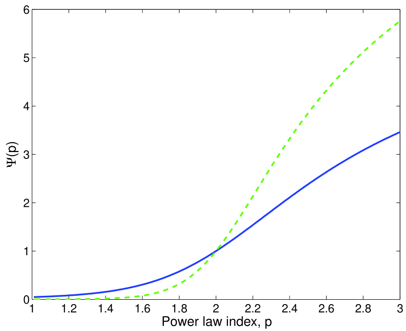
Figure 1.— Graph of the normalized function $\Psi(p)$ that determines the dependence of $\gamma_{\min}$ on the power law index $p$ of the accelerated electrons. Solid: $(\gamma_{\min}/\gamma_{\max})=10^{-3}$, dash: $(\gamma_{\min}/\gamma_{\max})=10^{-5}$ (see equation A.1).

A.2. Self absorption energy, $\varepsilon_{ssa}^{ob.}$

The synchrotron self absorption coefficient for a power law distribution of electrons with power law index $p$ radiating in magnetic field $B^{\prime}$ is calculated using standard formula (e.g., Rybicki & Lightman, 1979),

$$\alpha_{\nu}={\sqrt{27}q^{4}\over 16\pi^{2}m_{e}^{4}c^{5}}\left({3q\over 2\pi m_{e}^{3}c^{5}}\right)^{p/2-1}\left[{\Gamma\left({3p+2\over 12}\right)\Gamma\left({3p+22\over 12}\right)\over\Gamma\left({2\over 3}\right)\Gamma\left({7\over 3}\right)}\right]\Gamma\left({2\over 3}\right)\Gamma\left({7\over 3}\right)AB^{\prime p/2+1}\nu^{-(p/2+2)},$$ (A1)

where the constant $A$ is calculated using equation A.1,

$$A=u_{el}\times\left\{\begin{array}[]{ll}\log\left({\gamma_{\max}\over\gamma_{\min}}\right)^{-1}&(p=2),\\ {(p-2)\gamma_{\min}^{p-2}\over 1-\left({\gamma_{\min}\over\gamma_{\max}}\right)^{p-2}}&(p\neq 2),\end{array}\right.$$

which, upon insertion of $\gamma_{\min}$ can be written as

$$A=u_{el}\log\left({\gamma_{\max}\over\gamma_{\min}}\right)^{-1}\left({u_{el}\over\epsilon_{pl}n_{el}m_{e}c^{2}}\right)^{p-2}\left[{1-(\gamma_{\min}/\gamma_{\max})\over\log{\left({\gamma_{\max}\over\gamma_{\min}}\right)}}\right]^{p-2}\Psi^{p-2}(p)\xi(p),$$ (A2)

where

$$\xi(p)=\left\{\begin{array}[]{ll}1&(p=2),\\ {(p-2)\log\left({\gamma_{\max}\over\gamma_{\min}}\right)\over 1-\left({\gamma_{\min}\over\gamma_{\max}}\right)^{p-2}}&(p\neq 2).\end{array}\right.$$

Inserting the numerical values of the magnetic field and the peak frequency $\nu_{peak}=\varepsilon_{m}^{ob.}/\Gamma h$ (see equations 2, 2) into the self absorption coefficient equation A1, using the value of $A$ found in equation A2, one obtains the synchrotron self absorption coefficient at the peak frequency,

$$\begin{array}[]{ll}\alpha_{\nu_{peak}}=&1.56\times 10^{-11}\,L_{52}^{1/2}\,r_{13}^{-1}\Gamma_{2}^{-1}\,\epsilon_{e,-0.5}^{-5}\,\epsilon_{pl,0}^{6}\,\epsilon_{B,-0.5}^{-1/2}\,\theta_{p,0}^{-11/2}\,\zeta_{0}^{1/2}\\ &\times(3.0\times 10^{12})^{p/2-1}\left[{\Gamma\left({3p+2\over 12}\right)\Gamma\left({3p+22\over 12}\right)\over\Gamma\left({2\over 3}\right)\Gamma\left({7\over 3}\right)}\right]\xi(p)\Psi^{-6}(p)\,{\rm cm^{-1}}.\end{array}$$

The self absorption optical depth $\tau_{\nu}=\Delta r^{\prime}_{B}\alpha_{\nu}$ is smaller than unity at $\nu=\nu_{peak}$. Since (by demand) the electrons are in the slow cooling regime (i.e., $\gamma_{\min}\leq\gamma_{c}$), the power radiated per unit energy below $\varepsilon_{m}=\varepsilon_{m}^{ob.}/\Gamma$ is proportional to $(\varepsilon/\varepsilon_{m})^{1/3}$, and the energy below which the optical depth becomes greater than unity, $\varepsilon_{ssa}=\varepsilon_{m}\tau_{\nu=\nu_{peak}}^{3/5}$, is

$$\begin{array}[]{ll}\varepsilon_{ssa}^{ob.}=&{31\over 1+z}\,L_{52}^{4/5}\,r_{13}^{-8/5}\,\Delta{r^{\prime}}_{B,7}^{3/5}\,\Gamma_{2}^{-3/5}\,\epsilon_{e,-0.5}^{-1}\,\epsilon_{pl,0}^{8/5}\,\epsilon_{B,-0.5}^{1/5}\,\theta_{p,0}^{-4/5}\,\zeta_{0}^{4/5}\\ &\times(3.0\times 10^{12})^{(3/5)(p/2-1)}\left[{\Gamma\left({3p+2\over 12}\right)\Gamma\left({3p+22\over 12}\right)\over\Gamma\left({2\over 3}\right)\Gamma\left({7\over 3}\right)}\right]^{3/5}\xi^{3/5}(p)\Psi^{-8/5}(p)\,\rm{\,eV}\end{array}$$

(compare with equation 2). Therefore, the definition of the function $\chi(p)$ is

$$\chi(p)\equiv(3.0\times 10^{12})^{(3/5)(p/2-1)}\left[{\Gamma\left({3p+2\over 12}\right)\Gamma\left({3p+22\over 12}\right)\over\Gamma\left({2\over 3}\right)\Gamma\left({7\over 3}\right)}\right]^{3/5}\xi^{3/5}(p)\Psi^{-8/5}(p).$$ (A3)

This function is plotted in figure 2.

Inserting the parametric dependence on the value of $\Psi(p)$ of the four parameters found in equation (2) into equation A.2, leads to $\tilde{\chi}(p)=\chi(p)\times\Psi^{-19/10}(p)$. Graph of this function appears in figure 3. Note that while $\chi(p)$ shows a very strong dependence on the value of $p$, the function $\tilde{\chi}(p)$ varies by a factor less than 4 in the range $2\leq p\leq 2.4$.

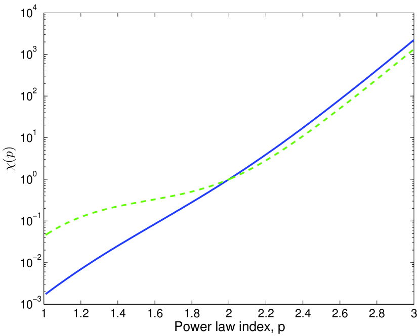
Figure 2.— Graph of the normalized function $\chi(p)$ that determines the dependence of $\epsilon_{ssa}^{ob.}$ on the power law index $p$ of the accelerated electrons. Solid: $(\gamma_{\min}/\gamma_{\max})=10^{-3}$, dash: $(\gamma_{\min}/\gamma_{\max})=10^{-5}$ (see equation 2).

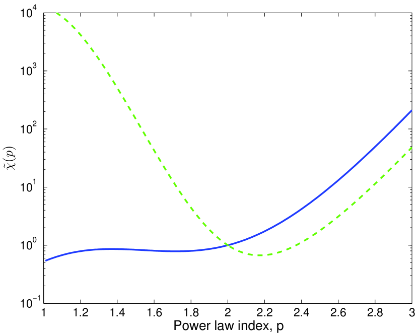
Figure 3.— Graph of the normalized function $\tilde{\chi}(p)$ that determines the dependence of $\varepsilon_{ssa}^{ob.}$ on the power law index $p$ of the accelerated electrons, for the parameters values derived from observations. Solid: $(\gamma_{\min}/\gamma_{\max})=10^{-3}$, dash: $(\gamma_{\min}/\gamma_{\max})=10^{-5}$ (see equation 3).

References

- Chevalier (1992) Chevalier, R. A. 1992, Nature, 355, 617
- Cohen et al. (1997) Cohen, E., et al. 1997, ApJ, 488, 330
- Crider et al. (1997) Crider, A., et al. 1997, ApJ, 479, L39
- Derishev et al. (2001) Derishev, E.V., Kocharovsky, V.V., & Kocharovsky, Vl, V. 2001, A&A, 372, 1071
- Dhawan et al. (2000) Dhawan, V., Mirabel, I.F., & Rodríguez, L.F. 2000, ApJ, 543, 373
- Fender (2003) Fender, R. 2003, in ’Compact Stellar X-Ray Sources’, eds. W.H.G. Lewin and M. van der Klis, Cambridge University Press (astro-ph/0303339)
- Frail et al. (2000) Frail, D.A, Waxman, E., & Kulkarni, S.R. 2000, ApJ, 537, 191
- Frederiksen et al. (2004) Frederiksen, J.T., et al. 2004, ApJ, 608, L13
- Freedman & Waxman (2001) Freedman, D.L., & Waxman, E. 2001, ApJ, 547, 922
- Frontera et al. (2000) Frontera, F., et al. 2000, ApJS, 127, 59
- Ghirlanda et al. (2003) Ghirlanda, G., Celotti, A., & Ghisellini, G. 2003, A& A, 406, 879
- Ghisellini & Celotti (1999) Ghisellini, G., & Celotti, A. 1999, ApJ, 511, L93
- Ghisellini et al. (2000) Ghisellini, G., Celotti, A., & Lazzati, D. 2000, MNRAS, 313, L1
- Gruzinov (2001) Gruzinov, A. 2001, ApJ, 563, L15
- Hededal et al. (2004) Hededal, C.B., et al. 2004, ApJ, 617, L107
- Jaroschek et al. (2004) Jaroschek, C.H., Lesch, H., & Treumann, R.A. 2004, ApJ, 616, 1065
- Kaneko et al. (2006) Kaneko, Y., et al. 2006, ApJS, in press (astro-ph/0605427)
- Katz (1994) Katz, J.I. 1994, ApJ, 432, L107
- Kazimura et al. (1998) Kazimura, Y., et al. 1998, ApJ, 498, L183
- Kumar et al. (2006) Kumar, P., et al. 2006, MNRAS, 367, L52
- Lazzati et al. (2000) Lazzati, D., Ghisellini, G., Celotti, A., & Rees, M.J. 2000, ApJ, 529, L17
- Liang (1997) Liang, E. P. 1997, ApJ, 491, L15
- Liang et al. (1997) Liang, E. P., Kusunose, M., Smith, I., & Crider, A. 1997, ApJ, 479, L35
- Lloyd & Petrosian (2000) Lloyd, N.M., & Petrosian, V. 2000, 543, 722
- Lloyd-Ronning & Petrosian (2002) Lloyd-Ronning, N.M., & Petrosian, V. 2002, ApJ, 565, 182
- Medvedev & Loeb (1999) Medvedev, M.V., & Loeb, A. 1999, ApJ, 526, 697
- Mészáros et al. (1993) Mészáros, P., Laguna, P., & Rees, M.J. 1993, ApJ, 415, 181
- Mészáros et al. (2002) Mészáros, P., Ramirez-Ruiz, E., Rees, M.J., & Zhang, B. 2002, ApJ, 578, 812
- Mészáros & Rees (1993a) Mészáros, P., & Rees, M.J. 1993, ApJ, 405, 278
- Mészáros & Rees (1993b) Mészáros, P., & Rees, M.J. 1993, ApJ, 418, L59
- Mészáros & Rees (1997) Mészáros, P., & Rees, M.J. 1997, ApJ, 476, 232
- Mészáros & Rees (2000) Mészáros, P., & Rees, M.J. 2000, ApJ, 530, 292
- Mészáros et al. (1994) Mészáros, P., Rees, M.J., & Papathanassiou, H. 1994, ApJ, 432, 181
- Nishikawa et al. (2005) Nishikawa, K.-I., et al. 2005, ApJ, 622, 927
- Osborne (2006) Osborne, J.P. 2006, private communication
- Page et al. (2005) Page, M. et al. 2005, GCN 3830
- Panaitescu & Kumar (2001) Panaitescu, A., & Kumar, P. 2001, ApJ, 560, L49
- Panaitescu & Kumar (2002) Panaitescu, A., & Kumar, P. 2001, ApJ, 571, 779
- Panaitescu & Mészáros (1998) Panaitescu, A., & Mészáros, P. 1998, ApJ, 501, 772
- Panaitescu & Mészáros (2000) Panaitescu, A., & Mészáros, P. 2000, ApJ, 544, L17
- Pe’er et al. (2005) Pe’er, A., Mészáros, P., & Rees, M.J. 2005, ApJ, 635, 476
- Pe’er et al. (2006) Pe’er, A., Mészáros, P., & Rees, M.J. 2006, ApJ, 642, 995
- Pe’er & Waxman (2004) Pe’er, A., & Waxman, E. 2004, ApJ, 613, 448
- Pe’er & Wijers (2006) Pe’er, A., & Wijers, R.A.M.J. 2006, ApJ, 643, 1036
- Piran (2005) Piran, T. 2005, preprint (astro-ph/0503060)
- Preece et al. (1998) Preece, R.D., et al. 1998, ApJ, 506, L23
- Preece et al. (2000) Preece, R.D., et al. 2000, ApJS, 126, 19
- Preece et al. (2002) Preece, R.D., et al. 2002, ApJ, 581, 1248
- Rees & Mészáros (1992) Rees, M.J., & Mészáros, P. 1992, MNRAS, 258, 41
- Rees & Mészáros (1994) Rees, M.J., & Mészáros, P. 1994, ApJ, 430, L93
- Romano et al. (2006) Romano, P., et al. 2006, preprint (astro-ph/0602497)
- Rossi & Rees (2003) Rossi, E., & Rees, M.J. 2003, MNRAS, 339, 881
- Rybicki & Lightman (1979) Rybicki, G.B., & Lightman, A.P. 1979, Radiative Processes in Astrophysics (New York: Wiley)
- Sari et al. (1996) Sari, R., Narayan, R. & Piran, T. 1996, ApJ, 473, 204
- Sari & Piran (1997) Sari, R., & Piran, T. 1997, MNRAS, 287, 110
- Sari et al. (1998) Sari, R., Piran, T., & Narayan, R. 1998, ApJ, 497, L17
- Schaefer et al. (1998) Schaefer, B.E., et al. 1998, ApJ, 492, 696
- Silva et al. (2003) Silva, L.O., et al. 2003, ApJ, 596, L121
- Tavani (1996a) Tavani, M. 1996, ApJ, 466, 768
- Tavani (1996b) Tavani, M. 1996, Phys. Rev. Lett., 76, 3478
- Waxman (1997a) Waxman, E. 1997, ApJ, 485, L5
- Waxman (1997b) Waxman, E. 1997, ApJ, 489, L33
- Wiersma & Achterberg (2004) Wiersma, J., & Achterberg, A. 2004, A&A, 428, 365
- Wijers & Galama (1999) Wijers, R.A.M.J., & Galama, T.J. 1999, ApJ, 523, 177
- Zhang & Mészáros (2002) Zhang, B., & Mészáros, P. 2002, ApJ, 581, 1236
- Zhang & Mészáros (2004) Zhang, B., & Mészáros, P. 2004, Int. J. Mod. Phys. A, 19, 2385