Shadows and Photoevaporated Flows from Neutral
Clumps Exposed to Two Ionizing Sources

Abstract

Neutral clumps immersed in HII regions are frequently found in star formation regions. We investigate here the formation of tail of neutral gas, which are not reached by the direct ionizing flux coming from two massive stars, using both an analytical approximation, that allows us to estimate the shadow geometry behind the clumps for different initial geometric configurations, and three-dimensional numerical simulations. We found a good agreement between both approaches to this theoretically interesting problem. A particularly important application could be the proplyds that are found in the Trapezium cluster in Orion, which are being photoevaporated primordially by the O stars $\theta^{1}$ Ori C and $\theta^{2}$ Ori A.

Glóbulos neutros sumergidos en regiones HII son frecuentemente encontrados en regiones de formación estelar. En este trabajo investigamos la formación de regiones de sombra detrás de glóbulos neutros iluminados por el flujo ionizante directo de dos estrellas. Utilizamos una aproximación analítica, la cual nos permite hacer estimaciones de la geometría de las sombras detrás de los glóbulos neutros para distintas configuraciones geométricas iniciales, y tambien simulaciones numéricas tridimensionales. Encontramos un buen acuerdo entre los cálculos analíticos y los numéricos. Una aplicación de particular relevancia pueden ser los proplyds ubicados en el cúmulo del Trapecio en Orión, los cuales están siendo fotoevaporados por la radiación de las estrellas O $\theta^{1}$ Ori C y $\theta^{2}$ Ori A.

hydrodynamics H II regions Stars: Pre-main sequence Stars: formation

0.1 Introduction

High density neutral clumps immersed in a bath of photoionizing and photodissociating radiation can be found in several regions in our own Galaxy. To quote only a few examples, we can find cometary globules like CG 1 in H II regions (in the Gum Nebula), for which the major source of ultra-violet (UV) photons is the Zeta Puppis star (e.g., Reipurth 1983); the proplyds found near the Trapezium cluster in Orion (e.g., O’Dell 1998; Bally et al. 1998), as well as in other H II regions with star formation (e.g., Smith et al. 2003). The morphology, dynamics and emission line spectrun of the Orion proplyds is explained as the photoevaporation of circumstellar disks by the ionizing photon flux that comes from $\theta^{1}$ Ori C (Johnstone et al. 1998; Richling & Yorke 2000). Another example of high density neutral condensations in an ionizing radiation field are Thackeray’s globules in the IC 2944 region, which show a fragmented, clumpy structure (Reipurth et al. 2003). We can also find high density clumps associated with planetary nebulae (PN). The Helix Nebula (NGC 7293, e.g., O’Dell & Handron 1996) displays thousands of cometary shaped neutral clumps, which are being photoevaporated (e.g., López-Martín et al. 2001) by the radiation field that comes from the central star. Attempts have also been made to reproduce observational aspects of the so-called Fast Low Ionization Emission Regions (or FLIERs) observed in a fraction of PN as a by-product of the photoevaporation of a neutral clump by the stellar radiation field (e.g., Mellema et al. 1998).

Previous analytical studies of high density neutral clumps exposed to an ionizing photon radiation field show that these systems have two distinct dynamical phases (e.g.; Bertoldi 1989; Bertoldi & McKee 1990; Mellema et al. 1998): an initial collapse (or radiation-driven implosion) phase and a cometary phase. The collapse phase starts when the ionizing photon flux reaches the clump surface, forming a D-type ionization front (IF). This IF is preceeded by a shock front, which propagates through the clump (at a velocity determined by the local isothermal sound speed) compressing, heating and accelerating the clump material. The ionized gas expands outwards (with a velocity approximately equal to the isothermal sound speed of the ionized material) generating a photoevaporated flow. The recombination of the gas downstream of the IF (i.e., in the photoevaporated flow) partially shields the clump surface from the ionizing photon flux that comes from the ionizing source, and this is also an important effect influencing the evolution of the collapse phase. When the shock front propagates through the entire clump, in a timescale given by $t_{0}=2R_{c}/v_{s}$ (where $R_{c}$ is the initial clump radius and $v_{s}$ is the shock speed), the clump starts to accelerate as a whole (as a dynamical response to the production of a photoevaporated flow; i.e., the rocket effect) and enters the cometary phase. The clump material is found to be completely ionized in a timescale that depends on both $t_{0}$ and the shielding of the impinging ionizing flux (e.g., see Mellema et al. 1998).

One of the first numerical studies of an ionizing radiation field interacting with a neutral clump was related to the problem of star formation. Klein et al. (1980) and Sandford et al. (1982) developed a two-dimensional code in order to numerically reproduce the interaction of an ionizing radiation field from (an already formed) OB star association with local inhomogeneities in a molecular cloud. These early studies were able to capture the radiation-driven implosion of the clump material. They have also found that the shock induced by the ionization front at the clump surface substantially increases the density when compared with an analytical, one-dimensional evaluation.

The subsequent evolution of these neutral clumps to the cometary regime was investigated numerically in two-dimensions by Lefloch & Lazareff (1994) and Mellema et al. (1998). In particular, the numerical simulations of a cometary globule carried out by Lefloch & Lazareff (1994) show that, after a short timescale ($\approx 10\%$ of the clump lifetime) associated with the collapse phase, the clump evolves to a situation of quasi-hydrostatic equilibrium, characteristic of the cometary phase (see also Bertoldi 1989). In a subsequent paper, Lefloch & Lazareff (1995) show that the cometary globule CG7S could be successfully explained as a neutral clump undergoing the collapse phase under the influence of a nearby group of O stars. On the other hand, Mellema et al. (1998) were able to reproduce the kinematic and emission properties of FLIERs seen in PN with a model of a clump, located in the outer parts of a PN, being photoionized by the central PN star. They have also been able to follow the onset of the collapse phase and its photoevaporated flow, the effect of the photoevaporated flow on the clump shaping, and the further acceleration of the clump in the cometary phase. More recently, three-dimensional numerical simulations of non-uniform high density clumps (González et al. 2005) subject also to the influence of a wind (Raga et al. 2005) have been carried out. These effects are important for the study of proplyds as well as for Thackeray’s globules.

The observed high density neutral structures associated with H II regions and PN, project a shadow away from the direction of the impinging ionizing photon flux. Cantó et al. (1998) studied the shape and structure of the shadow projected by a spherical clump in a photoionized region, also taking into account the effect of the diffuse ionizing field. They were able to describe (analytically and numerically) the transition between a shadow region that is optically thin to the diffuse ionizing radiation field to a neutral inner core inside the shadow. They also predicted that the H$\alpha$ emission coefficient is substantially greater in the shadow region when compared with the surrounding H II region (and, then, to conclude that the shadow should be brighter than the H II region). A similar approach was followed by Pavlakis et al. (2001), who carried out 2-D simulations. They found that if the diffuse ionizing field is 10% of the direct field, the evolution of the clump is considerably different to the evolution of the clump without the diffuse radiation field. Nevertheless, none of these papers have attempted to follow the whole evolution of the shadow as the clump evolves from the collapse through the cometary phases.

Observationally, some photoionized neutral structures (for example, the Orion proplyds, see O’Dell 1998) have relatively short elongations of neutral material into the shadow region, while others have extremely long “tails” extending away from the photoionizing source. Examples of long tails are the cometary knots in the Helix nebula (see, e.g., the recent paper of O’Dell, Henney & Ferland 2005) and the dark trails which cut through the outer regions of M 42 (O’Dell 2000). In these tail regions, one has a combination of the shadowing effect and the photoionization due to the diffuse radiation (see Cantó et al. 1998 and Pavlakis et al. 2001) as well as the possible presence of a photodissociated wind coming from the back side of the neutral clump or disk structure (as has been explored for the case of the Orion proplyds by Richling & Yorke 2000).

An interesting effect is that neutral clumps in H II regions in some cases are being photoionized by the radiation from more than one star. For example, the structures of some of the proplyds appear to be affected not only by the radiation from $\theta^{1}$ Ori C, but also by $\theta 2$ Ori A (in particular the 197-427, 182-413 and 244-440 proplyds, see O’Dell 1998 and Henney & O’Dell 1999). A possibly more complex example are the proplyds in the Carina nebula (Smith et al. 2003), which are possibly affected by the radiation from several stars in the neighborhood. This situation was first addressed by Klein, Sanford and Whitaker (1983), who performed two-dimensional radiation-hydrodynamics calculations of the interaction of the radiation field from two massive stars with a neutral clump, in order to investigate whether or not such a system could trigger star formation within OB subgroups. The calculation performed by Klein et al. considered two identical stars (separated by 1 pc) and, in the middle of the straight line connecting both stars, a neutral clump (with a radius of 0.6 pc). They found that the clump is strongly compressed (by a factor of 170) after its implosion and reaches the Jeans mass at some points (located in a torus that surrounds the clump initial position) in a time scale smaller than that in which the clump can be photo-evaporated. Thus, they conclude that stars could be formed in OB associations by this ”multiple implosion mechanism”.

In the present paper, we investigate the evolution of a high density neutral clump subject to the influence of two ionizing photon sources. In some sense, this paper represents a generalization of the Klein et al. (1983) work, since they only studied the axysimmetric case in which the stars and the clump are aligned . We first present an analytical description of the shape of the shadow behind the clump considering both the distance from the sources as well as their angular displacement. A set of three-dimensional numerical simulations is also presented, in which we follow the evolution of the shadows as well as the clump radius and neutral mass.

This paper is planned as follows. In §2, we present an analytical solution for the shape of the shadows behind a clump illuminated by two sources. In §3, we explore the parameters numerically and we present the results of three-dimensional numerical simulations of this problem. In §4, the discussions and conclusions are presented.

0.2 Shadows behind illuminated clumps

Figure 1: Schematic diagram showing i) the relation between the two coordinate systems, $O$ and $O^{\prime}$, ii) the clump represented by a sphere of radius $R_{c}$ (projected onto the $yz-$plane), iii) the angles $\alpha$ and $\beta$ and iv) the distance from the star $R_{\star}$. See the text for a discussion.

Figure 1 defines two frames of reference $O$ and $O^{\prime}$. Both frames have their origins at the center of a spherical clump of radius $R_{c}$, and the star is on the $yz-$ and $y^{\prime}z^{\prime}-$ planes. Frame $O$ has an arbitrary orientation, while frame $O^{\prime}$ is oriented such that its $z^{\prime}$-axis is along the line joining the center of the clump with the star. The star is located at a distance $R_{\star}$ from the clump and has coordinates: $x=0$, $y=-R_{\star}{\rm sin}\alpha$ and $z=-R_{\star}{\rm cos}\alpha$ in frame $O$; and $x^{\prime}=0$, $y^{\prime}=0$ and $z^{\prime}=-R_{\star}$ in frame $O^{\prime}$ (see Figure 1). The half opening angle $\beta$ of the shadow cone is given by:

Figure 2: Schematic diagram showing the relative position, angles and distance between the two stars and the clump. See the text for a discussion.

$${\rm sin}\beta=\frac{R_{c}}{R_{\star}}.$$ (1)

Thus the width $\omega$ of the shadow cone increases as,

$$\omega={\rm tan}\beta(R_{\star}+z^{\prime})=\frac{R_{c}}{(R_{\star}^{2}-R_{c}^{2})^{1/2}}(R_{\star}+z^{\prime}).$$ (2)

The shadow cone is tangent to the clump at,

$$z_{c}^{\prime}=R_{c}{\rm sin}\beta,\leavevmode\nobreak\ \leavevmode\nobreak\ \leavevmode\nobreak\ y_{c}^{\prime}=R_{c}{\rm cos}\beta,$$ (3)

thus the shadow region behind the clump is given by,

$$(x^{\prime 2}+y^{\prime 2})^{1/2}\leq\omega={\rm tan}\beta(R_{\star}+z^{\prime}),$$ (4)

and

$$z^{\prime}\geq z_{c}^{\prime}=-R_{c}{\rm sin}\beta,$$ (5)

where the equal sign in (4) corresponds to the boundary of the shadow.

The coordinate transformation equations between frames $O$ and $O^{\prime}$ are,

$$x^{\prime}=x,\leavevmode\nobreak\ \leavevmode\nobreak\ \leavevmode\nobreak\ \leavevmode\nobreak\ \leavevmode\nobreak\ \leavevmode\nobreak\ \leavevmode\nobreak\ \leavevmode\nobreak\ \leavevmode\nobreak\ \leavevmode\nobreak\ \leavevmode\nobreak\ \leavevmode\nobreak\ \leavevmode\nobreak\ \leavevmode\nobreak\ \leavevmode\nobreak\ \leavevmode\nobreak\ \leavevmode\nobreak\$$

$$y^{\prime}=y\,{\rm cos}\alpha-z\,{\rm sin}\alpha,$$ (6)

$$z^{\prime}=y\,{\rm sin}\alpha+z\,{\rm cos}\alpha.$$

Substituting (0.2) in (4) and (5) we find that the shadow region in frame $O$ is,

$$[x^{2}+(y\,{\rm cos}\alpha-z\,{\rm sin}\alpha)^{2}]^{1/2}\leq\leavevmode\nobreak\ \leavevmode\nobreak\ \leavevmode\nobreak\ \leavevmode\nobreak\ \leavevmode\nobreak\ \leavevmode\nobreak\ \leavevmode\nobreak\ \leavevmode\nobreak\ \leavevmode\nobreak\ \leavevmode\nobreak\ \leavevmode\nobreak\ \leavevmode\nobreak\ \leavevmode\nobreak\ \leavevmode\nobreak\ \leavevmode\nobreak\ \leavevmode\nobreak\ \leavevmode\nobreak\ \leavevmode\nobreak\$$

$$\frac{R_{c}}{(R_{\star}^{2}-R_{c}^{2})^{1/2}}(R_{\star}+z\,{\rm cos}\alpha+y\,{\rm sin}\alpha),$$ (7)

and

$$y\,{\rm sin}\alpha+z\,{\rm cos}\alpha\geq-\frac{R_{c}^{2}}{R_{\star}}.$$ (8)

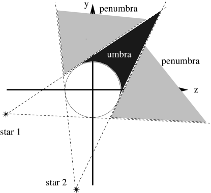
Figure 3: Schematic diagram showing the umbra and the penumbra regions in the shadow behind a clump illuminated by two stars.

Consider the case of a clump illuminated by two stars, one located at a distance $R_{1}$ at an angle $\alpha_{1}$ and the other at a distance $R_{2}$ with an angle $\alpha_{2}$. The $yz-$plane contains both stars and the center of the clump (see Figure 2). The shadow produced by the two stars is divided in two regions. One, the umbra where the light from both stars is blocked by the clump, and the other, the penumbra where only the light from one of the stars is shaded by the clump (see Figure 3).

In the $yz-$plane ($x=0$) the boundary of the shadows are straight lines given by (see eq. 0.2),

$$y\,{\rm cos}\alpha_{1}-z\,{\rm sin}\alpha_{1}=\pm{\rm tan}\beta_{1}(R_{1}+z\,{\rm cos}\alpha_{1}+y\,{\rm sin}\alpha_{1})$$ (9)

for star 1, and,

$$y\,{\rm cos}\alpha_{2}-z\,{\rm sin}\alpha_{2}=\pm{\rm tan}\beta_{2}(R_{2}+z\,{\rm cos}\alpha_{2}+y\,{\rm sin}\alpha_{2})$$ (10)

for star 2, where,

$${\rm tan}\beta_{1}=\frac{R_{c}}{(R_{1}^{2}-R_{c}^{2})^{1/2}}\leavevmode\nobreak\ \leavevmode\nobreak\ {\rm and}\leavevmode\nobreak\ \leavevmode\nobreak\ {\rm tan}\beta_{2}=\frac{R_{c}}{(R_{2}^{2}-R_{c}^{2})^{1/2}}{\rm.}$$ (11)

Assuming that $\alpha_{2}>\alpha_{1}$, then the maximum extent of the umbra $R_{0}$ (see Figure 2) is given by the intersection of lines (9) (with the plus sign) and line (10) (with the minus sign). The coordinates of the intersection point are,

$$x_{0}=0,\leavevmode\nobreak\ \leavevmode\nobreak\ y_{0}=R_{0}{\rm sin}\alpha_{0}\leavevmode\nobreak\ \leavevmode\nobreak\ {\rm and}\leavevmode\nobreak\ \leavevmode\nobreak\ z_{0}=R_{0}{\rm cos}\alpha_{0}{\rm,}$$ (12)

where

$$R_{0}=\frac{R_{c}}{{\rm sin}\gamma},$$ (13)

and

$$\alpha_{0}=\frac{(\alpha_{1}+\alpha_{2})-(\beta_{2}-\beta_{1})}{2},$$ (14)

$$\gamma=\frac{(\alpha_{2}-\alpha_{1})-(\beta_{1}+\beta_{2})}{2}.$$ (15)

The geometrical interpretation of $\alpha_{0}$ and $\gamma$ is shown in Figure 2.

It follows from (13) that $R_{0}\rightarrow\infty$ and $\gamma\rightarrow 0$, for $(\alpha_{2}-\alpha_{1})\rightarrow(\beta_{1}+\beta_{2})$. Therefore for $(\alpha_{2}-\alpha_{1})<(\beta_{1}+\beta_{2})$ the umbra is not bounded and it extends to infinity.

Let us define a function $J(x,y,z,\alpha,R_{\star})$ such that $J=1$ if (0.2) and (8) are satisfied and $J=0$ otherwise. Then, for the umbra $J(x,y,z,\alpha_{1},R_{1})=1$ and $J(x,y,z,\alpha_{2},R_{2})=1$ while for the penumbra either $J(x,y,z,\alpha_{1},R_{1})=0$ and $J(x,y,z,\alpha_{2},R_{2})=1$ or $J(x,y,z,\alpha_{1},R_{1})=1$ and $J(x,y,z,\alpha_{2},R_{2})=0$. In the region illuminated by both stars $J(x,y,z,\alpha_{1},R_{1})=0$ and $J(x,y,z,\alpha_{2},R_{2})=0$.

There is one case of particular interest, that in which both $R_{1}$ and $R_{2}$ are much greater than $R_{c}$, and that we will explore in the next section numerically. In the limit, $(R_{c}/R_{1})$ and $(R_{c}/R_{2})\rightarrow 0$, both $\beta_{1}$ and $\beta_{2}\rightarrow 0$ and thus [see (14) and (15)],

$$\alpha_{0}=\frac{(\alpha_{1}+\alpha_{2})}{2}\leavevmode\nobreak\ \leavevmode\nobreak\ {\rm and}\leavevmode\nobreak\ \leavevmode\nobreak\ \gamma=\frac{(\alpha_{2}-\alpha_{1})}{2}{\rm,}$$ (16)

with $R_{0}$ given by (13).

To get an idea of the shape of the umbra in this case let us consider a particular orientation of our frame of reference. This orientation is such that

$$\alpha_{2}=\pi-\alpha_{1}\,.$$ (17)

Then, from (16),

$$\alpha_{0}=\frac{\pi}{2}\leavevmode\nobreak\ \leavevmode\nobreak\ {\rm and}\leavevmode\nobreak\ \leavevmode\nobreak\ \gamma=\frac{\pi}{2}-\alpha_{1},$$ (18)

and from (13),

$$R_{0}=\frac{R_{c}}{{\rm cos}\alpha_{1}}.$$ (19)

The boundary of the shadow projected by each star is [see (0.2)],

$$x^{2}+(y\,{\rm cos}\alpha_{1}-z\,{\rm sin}\alpha_{1})^{2}=R_{c}^{2}$$ (20)

for star 1, and,

$$x^{2}+(y\,{\rm cos}\alpha_{2}-z\,{\rm sin}\alpha_{2})^{2}=R_{c}^{2}$$ (21)

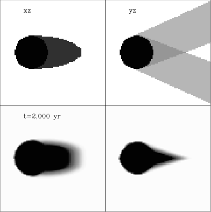
Figure 4: Top: A spherical clump and its projected umbra and penumbra on the $xz$- (left) and $yz$-planes (right), assuming that the two stars are on the $yz$-plane. Bottom: Maps of the ionization fraction at the beggining of the calculation ($t=2\,000$ years). As in the previous maps, a spherical clump creates a shadow on the $xz$- (left) and $yz$-planes (right). In all cases, the abscissa corresponds to the $z$-coordinate and is limited by $40<z<130$, and the ordinate corresponds to the $x$ (left) or $y$ (right), both limited by $19<x,y<109$ (in units of $7.8\times 10^{15}$ cm).

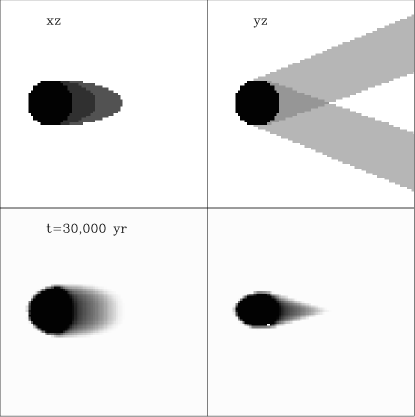
Figure 5: The same as in Figure 4, but for a more evolved temporal stage ($t=30\,000$ years). In all cases, the abscissa corresponds to the $z$-coordinate and is limited by $80<z<170$ (as the clump is accelerated towards the positive $z$ direction; see §3 below), and the ordinate corresponds to the $x$ (left) or $y$ (right), both limited by $19<x,y<109$ (in units of $7.8\times 10^{15}$ cm).

for star 2. Solving (20) and (21) simultaneously and using (17) it follows that the condition for the intersection of the boundaries is $z=0$. That is, the shadows intersect at the plane $z=0$, which is consistent with the value of $\alpha_{0}=\pi/2$ [see (18)]. In this plane, the shape of the umbra is then,

$$x^{2}+y^{2}{\rm cos}^{2}\alpha_{1}=R_{c}^{2},$$ (22)

which represents an ellipse centered at the center of the clump with semi-axes $R_{c}$ in the $x$-direction and $R_{0}=R_{c}/{\rm cos}\alpha_{1}$ in the $y$-direction.

In order to compare the results from these analytical solutions with those from the numerical simulations, let us anticipate here some results before starting to discuss the simulations in detail in the next section. Although we have explored different angular distributions of these two stars with respect to the clump position, let us take here the case in which $2\gamma=45^{\circ}$ (see Figure 2), and a distance from the clump to the two stars of $d=3.6\times 10^{18}$ cm. This situation corresponds to model M45 discussed in the next section (see below). In Figure 4, we show both the analytical solution for the shadow geometry (top) and the ionization fraction (which should trace the shadow behind the clump) obtained through fully 3-D numerical simulations (bottom) of model M45. Also, Figure 4 shows the shadows on the $xz$- (left) and $yz$-plane (right). The stars and the clump are on the $yz$-plane. We note that there is a good agreement between the predicted geometry for the shadow (top-diagrams) compared with the ones obtained from the simulations (bottom-diagrams). As the simulations progress in time, the clump is photoevaporated and assumes a non-spherical shape, which can be seen in the bottom-diagrams of Figure 5. Such a departure from a spherical shape produces small differences between the predicted (see top-diagrams in Figure 5) and the simulated shadow geometry.

0.3 The numerical simulations

0.3.1 The numerical method and the simulations

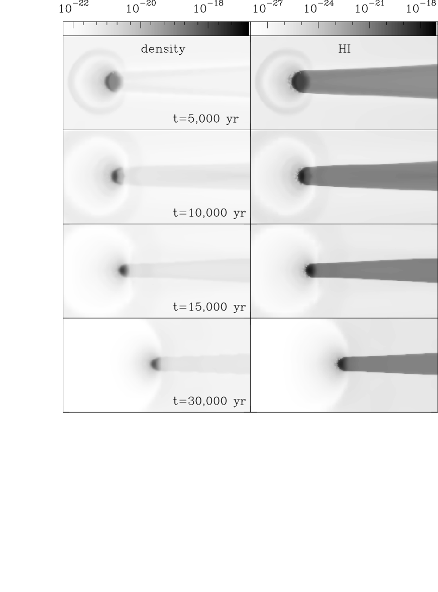
Figure 6: Distribution on the $yz-$plane of the total (left) and hydrogen neutral densities (right) for model M0 (see Table 1) at $t=5,000$, 10,000, 15,000 and 30,000 years (from top to bottom). The bars on the top give the scale in g cm^-3. The ionizing front comes from the left part of the computational domain (the ionizing sources are not depicted here).

In order to investigate the temporal behavior of the shadows of neutral (or partially neutral) material behind the clump exposed to two ionizing sources, we have carried out a set of three-dimensional numerical simulations. The simulations were performed using the Yguazú-a code. The Yguazú-a code, a binary adaptive grid code (see, e.g., Raga et al. 2000, 2002), has been extensively used in the literature, and has been tested against analytical solutions and laboratory experiments (see, e.g., Raga et al. 2000; Sobral et al. 2000; Raga et al. 2001; Velázquez et al. 2001; Raga & Reipurth 2004). The Yguazú-a code integrates the gas-dynamic equations (employing the “flux vector splitting” scheme of Van Leer). The code also solves rate equations for neutral/ionized hydrogen, and the radiative transfer of the direct photons at the Lyman limit (see González & Raga 2004).

We have computed models assuming a high density ($n_{c}=5\times 10^{4}$), low temperature clump ($T_{c}=10$ K) immersed in a low density ($n_{e}=100$ cm ^-3), high temperature environment ($T_{e}=1000$ K). All the models assume a clump of radius $r_{c}=10^{17}$ cm located at 1 parsec from the ionizing sources. The ionizing sources were assumed to have a black-body spectrum with an effective temperature of $T_{\star}={5\times 10^{4}}$ K and an emission rate of ionizing photons of $S_{\star}=1.5\times 10^{49}$ s^-1. In all models, the computational domain is limited to $x$, $y=10^{18}$ cm, $z=2\times 10^{18}$ cm and a 5-level binary adaptative grid with a maximum resolution of $7.81\times 10^{15}$ cm along each axis has been used. The centre of the clump is initially located at $x=y=z=5\times 10^{17}$ cm.

3 Model $\theta$ (^∘) $S_{1}$ ($s^{-1}$) $S_{2}$ ($s^{-1}$) M0 0 $1.50\times 10^{49}$ $1.50\times 10^{49}$ M45 45 $1.50\times 10^{49}$ $1.50\times 10^{49}$ M45b 45 $1.50\times 10^{49}$ $1.50\times 10^{48}$ M90 90 $1.50\times 10^{49}$ $1.50\times 10^{49}$

Table 1: The simulated models

In order to explore the geometrical effect on the shadows due to the presence of two ionizing sources, we have computed models with distinct relative angles between the clump and the two sources. In Table 1 we give the angles $\theta$, which are equivalent to $2\gamma$ as previously defined in Figure 2 (see also equations 15 and 16). In particular $\theta=0$ for model M0, $\theta=45^{\circ}$ for model M45 and $\theta=90^{\circ}$ for model M90 (see Table 1). We also note that we have conducted simulations with different ratios between the ionizing fluxes from the two sources, $F=S_{\star,1}/S_{\star,2}$, namely, $F=1$, and 10 (with $S_{\star,1}=1.5\times 10^{49}$ s^-1) . In the next section, we will discuss in detail the results from these numerical experiments.

0.3.2 Results

Figure 7: The same as in Figure 6, but for model M45 (see Table 1).

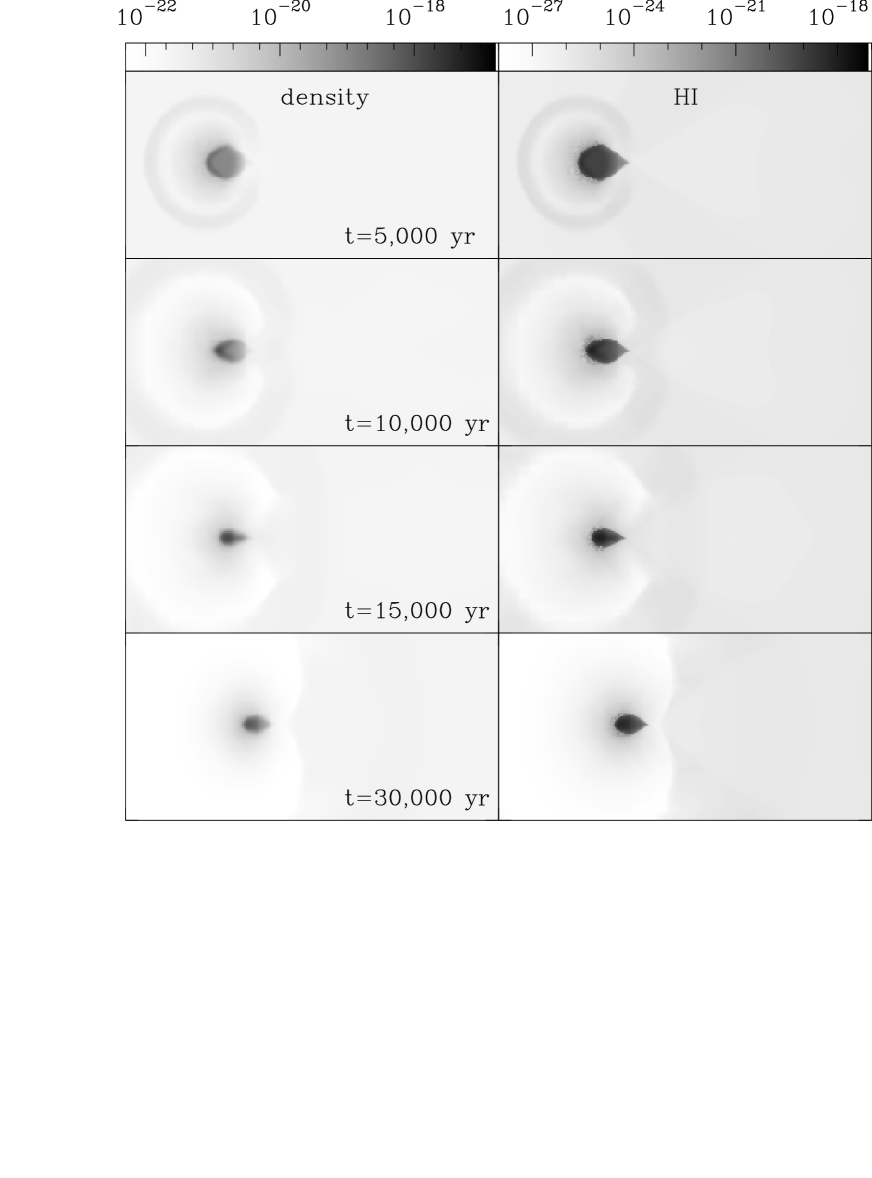
Figure 8: The same as in Figure 6, but for model M90 (see Table 1).

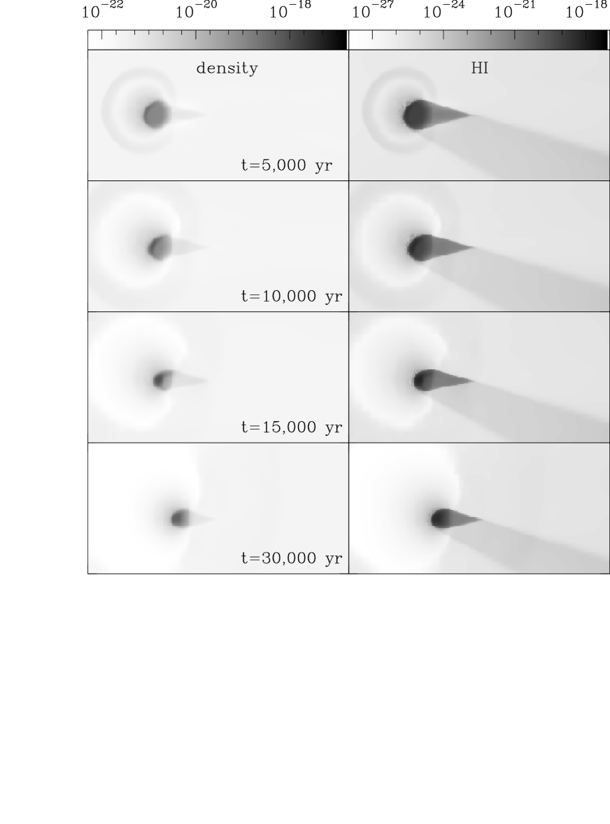
Figure 9: The same as in Figure 6, but for model M45b (see Table 1).

Figures 6, 7 and 8 show the temporal evolution of the total density (left) and the neutral hydrogen density (HI; right) for models M0, M45 and M90, respectively (see Table 1) at $t=5,000$, 10,000, 15,000 and 30,000 years. In these density distribution maps, we can identify i) a tail that fills the shadow region behind the clump (the umbra in Figure 3), ii) the emergence of a photoevaporated flow (that propagates towards the ionizing sources), and iii) the acceleration of the clump due to the rocket-effect.

As discussed in §2, the umbra is expected to have an extension $R_{0}$, which is in turn controlled by two parameters, namely, the clump radius $R_{c}$ and the relative angle $\gamma$ with respect to the sources (see equation 13 and Figure 2). In particular, the simulations show that the tail which appears in the shadow region behind the clumps has a cylindrical shape for model M0 ($R_{0}\rightarrow\infty$; Fig. 6), while in models M45 and M90 the umbra depicts a conical shape (see Figures 7 and 8). The conical umbra, however, is somewhat smaller in model M90 when compared with the one of model M45. We also note that the the cone height $R_{0}$ is actually a function of time ($R_{0}=R(t)$), since the photoevaporation of the clump material reduces the clump radius (see the discussion below). In all cases, both the umbra and the penumbra are completely symmetric with respect to the $z$-axis.

The photoevaporated flow can be seen in both the total density and HI density maps in Figures 6, 7 and 8. It expands almost radially from the clump position with a velocity $\lesssim 20$ km s^-1, producing density perturbations in the environment (a shock wave). This photoevaporated flow accelerates outwards, towards the ionizing photon sources. As a consequence, the clump itself is accelerated in the opposite direction. This effect is clearly seen in Figures 6, 7 and 8, where the clump is continuously pushed towards larges distances from the ionizing sources. However, we also note that the mass flux in the photoevaporated flow is smaller in model M90 than in model M45, and, as a consequence, the acceleration of the clump is also lower (see the discussion below).

In Figure 9 we show the evolution of the total density (left) and the neutral hydrogen density (HI; right) for model M45b (see Table 1) at $t=5,000$, 10,000, 15,000 and 30,000 years. We note that in this particular model, in which the ionizing sources have different ionizing photon rates ($S_{\star,1}/S_{\star,2}=10$), both the photoevaporated flow and the shadows behind the clump, particularly the penumbra, are not symmetric with respect to the $x$-axis. In particular, the photoevaporated flow is stronger in the direction of the most powerful ionizing source, $S_{1}$ (located towards the top-left direction of the diagram; see Figure 9). This causes a more pronounced ablation of the clump material that is facing the more powerful ionizing source. Also, only the penumbra of the shadow produced by the ionizing field from $S_{1}$ is seen.

Figure 10: a) Clump centre of mass (CM) position (measured by $Z_{CM}$, in units of $10^{17}$ cm) as a function of time for models M0 (full line), M45 (dotted line), M45b (dashed line) and M90 (dot-dashed line) (see Table 1). We note that the variations in $X_{CM}$ and $Y_{CM}$ are almost null for all models with the exception of M45b, see the discussion in the text. b) Velocity of the clump centre of mass ($V_{CM}$; in units of km s^-1) as a function of time (the curves are labeled in the top panel). c) Clump mass (normalized by the initial clump mass, $M_{c,0}=4.55\times 10^{32}$ g) as a function of time (the curves are labeled in the top panel). d) Clump radius (normalized by the initial clump radius, $R_{c,0}=10^{17}$ cm) as a function of time (the curves are labeled in the top panel). e) Shadow parameter $R_{0}$ (see equation 13), normalized by the initial clump radius, as a function of time (we note that $R_{0}\rightarrow\infty$ for model M0; not shown here).

In Figures 10a and 10b we show, respectively, the position $Z_{CM}$ of the center of mass of the clump and its velocity as a function of time (in years), for models M0 (full line), M45 (dotted line), M45b (dashed line) and M90 (dot-dashed line). As mentioned before, the clump in model M0 is rapidly accelerated (when compared with the clump in the other models) and attains large distances from the ionizing sources at shorter times. This is due to the fact that the mass loss rate associated with the photoevaporated flow, $\dot{M_{c}}$, is higher in this case. This is illustrated in Figure 10c, where the clump mass (normalized by the initial clump mass, $M_{c}(t=0)=M_{c,0}=\rho_{0}(4\pi/3)R_{c,0}^{3}=4.55\times 10^{32}$ g) is shown for all models, as a function of time. Note that the clump mass loss in the M0 model is higher (when compared with the other models).

Figure 11: Top: Clump centre of mass (CM) position (measured by $Z_{CM}$, in units of $10^{17}$ cm) as a function of time for simulated model M0 (full line; the same as in Figure 10). Also depicted in this figure is the result from the analytical approximation (diamonds) from Mellema et al. (1998), using as input parameters the sound speed $c_{0}$ and $c_{i}$ taken from the numerical simulation (see the text). Bottom: Clump mass (normalized by the initial clump mass, $M_{c,0}=4.55\times 10^{32}$ g) as a function of time taken from the M0 model (full line; the same as in Figure 10) . As in the previous diagram, the diamonds represents the analytical solution.

In Figure 10d we also show the spherical clump radius $R_{c}$ (normalized by the initial clump radius, $R_{c}(t=0)=R_{c,0}=10^{17}$ cm), as a function of time, for all of the models listed in Table 1. All of the curves show an almost monotonic behaviour. Note that the clump radius in model M0 is always smaller than the values obtained from the other models (which is consistent with the higher $\dot{M_{c}}$ of model M0). The temporal variation of the clump radius is responsible for the temporal variation of the height of the conical shadow $R_{0}$, as can be seen in figures 7, 8 and 9. In Fig. 10e, the height of the conical shadow $R_{0}$ (normalized by the initial clump radius, $R_{c,0}$; $R_{0}\rightarrow\infty$ for model M0, not shown in Figure 10e) is calculated using the clump radius given in Fig. 10d and equation (13). Note that, after a strong variation at the beginning ($t\lesssim 10^{4}$ years), the conical height tends to values $\approx R_{0}(t=0)/2$ in all models.

We have also compared the results from our simulations with results obtained from the analytical approximations given by Mellema et al. (1998). In that paper, the authors studied both the collapse (or implosion) and the cometary phases of a clump being exposed to an incident plane-parallel ionizing front (the case of model M0 here), and the mass and the position of the clump as a function of time have been derived for both phases. Using values obtained from our simulations for model M0 (following the notation in Mellema et al.: sound speed at the base of the photoevaporated flow, $c_{i}\simeq 8.64$ km s^-1; sound speed of the shocked gas inside the clump, $c_{0}\simeq 2.12$ km s^-1), we found that the collapse phase takes $t_{0}=13\,234$ years. Interestingly, almost all the curves in Figure 10 seems to change their behavior at this time, and this seems to be due to the end of this phase and the beginning of the cometary phase. At time $t_{0}$, the clump is predicted to have a mass $M_{c}\simeq 0.797\times M_{c,0}$. Figure 10c shows that model M0 has a mass at this time that is $\sim$ 10% smaller than this value, in good agreement with the analytic theory. Finally, the behavior of the solid curves in Figure 10a,c has also been compared with the solutions presented by Mellema et al. (1998) and a very good agreement is found between the values from the simulations and those predicted by the analytic theory during all of the evolution of the clump in model M0.

In particular, in Figure 11 we plot again the result from model M0 (full lines) and its comparison with the result from the analytical approximation from Mellema et al. (1998) (diamonds). Although the clump CM position is well recovered in the simulation (top panel), it seems that the mass of the clump is under-estimated in the numerical simulation when compared with the analytical solution. However, even in this case, both curves (full line and diamonds, on the bottom panel of Figure 11) depicts the same behavior. We have also simulated this same model M0, but with a grid-resolution of 512x128x128 (these numbers corresponding to a uniform grid at the highest resolution of our adaptative grid), or a grid spacing of $3.9\times 10^{15}$ cm (i. e., an improvement of a factor 2 with respect to the simulations that we have presented up to now). As in the previous, low resolution case, the CM position is well reproduced by the numerical simulation (not shown here), and the same under-estimation of the clump mass is also obtained.

0.4 Conclusions

In this paper, we have explored analytically what is the shape of the shadow behind a clump exposed to two ionizing photon sources. For the case in which the clump radius is much smaller than the distances to the sources, an analytical solution for the shapes of the umbra and the penumbra are found. We have also carried out 3D numerical simulations of this scenario, and we present four models with different relative positions between the two stars and the clump as well as with different combinations of ionizing photon rates for the sources.

These models show that the long neutral tails produced in the interaction of a neutral clump with a single photoionizing source (model M0, see Table 1 and Figure 4) disappear for the case of two angularly separated photoionizing sources producing comparable ionizing photon fluxes at the position of the clump (models M45 and M90, see Figures 5 and 6). This shortening of the neutral tails is again obtained in a model in which the ionizing photon fluxes from the two sources differ by a factor of 10 (model M45b, see Table 1 and Figure 7). In our numerical simulations, we also obtain the time-evolution of the cometary clump as it is accelerated away from the photoionizing sources by the rocket effect.

The present models are meant as an illustration of the effects of the interaction of a neutral clump with two photoionizing sources, which might be applicable to neutral structures in H II regions with several massive stars (see, e.g., O’Dell 1998; Smith et al. 2003). However, in our simulations we have not included the diffuse ionizing radiation (which might have an important effect on the shadow region, in particular in the case of ionization bounded nebulae) and the effect of the dissociative, direct and diffuse radiation (which can affect both the head and the tail regions, see Richling & Yorke 2000). In order to model the structure of specific clumps, these effects should also be included.