A Method To Remove Fringes From Images Using Wavelets

Abstract

We have developed a new method that uses wavelet analysis to remove interference fringe patterns from images. This method is particularly useful for flat fields in the common case where fringes vary between the calibration and object data. We analyze the efficacy of this method by creating fake flats with fictitious fringes and removing the fringes. We find that the method removes 90% of the fringe pattern if its amplitude is equal to the random noise level and 60% if the fringe amplitude is $\approx 1/10$ of the noise level. We also present examples using real flat field frames. A routine written in the Interactive Data Language (IDL) that implements this algorithm is available from the authors and as an attachment to this paper.

1. INTRODUCTION

The current class of telescopes with primary mirrors larger than $\sim$8 m in diameter allows researchers attainment of unprecedentedly high signal-to-noise ratios. In addition, ever-increasing computer capabilities have permitted quantitative analyses able to distinguish trends weaker than the noise level. This has not only allowed observations of fainter objects, but also observations of weak sources spatially indistinguishable from a bright source, such as the spectrum of an extrasolar planet orbiting a main-sequence star. In such cases, systematic errors that would not have been of importance when analyzing the bright source are of concern when considering the fainter source. Previously ignored systematic errors thus require algorithms able to correct them.

One such systematic effect is the appearance of fringes in data arrays. The strength of these fringes varies from instrument to instrument; we have seen it range from less than a tenth of the noise amplitude to roughly 5 times the noise amplitude.

Fringe correction methods found in the literature are either specific to the instrument or assume a global fringe period (e.g., Malumuth et al. 2003a, b; Mellau & Winnewisser 1995). The latter correction type makes uses of Fourier filtering, a technique that is less than satisfactory in the common case where the pattern’s period or amplitude varies over the image. Another common approach has simply been to ignore the fringes in the hope that division of the debiased data array by the flat field frame will eliminate the pattern, which was supposed to remain the same. However, flat fields and object frames do not always share the same fringe pattern because flexure and variations in the illumination geometry can change the pattern’s amplitude or period even on short timescales (Figs. 1 and 2). Therefore, flat-field division could add a second set of fringes rather than correct the first set.

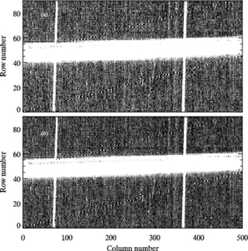
Figure 1.— Failure of flat field to correct fringes. Top: Debiased spectrum frame. Bottom: Spectrum frame after flat field and bias correction. The fringe pattern is still visible. These images are subsections of a spectrum frame obtained with NIRSPEC at the Keck telescope. The horizontal white pattern is the spectrum’s trace. Bright, white, vertical lines are the sky emission lines.

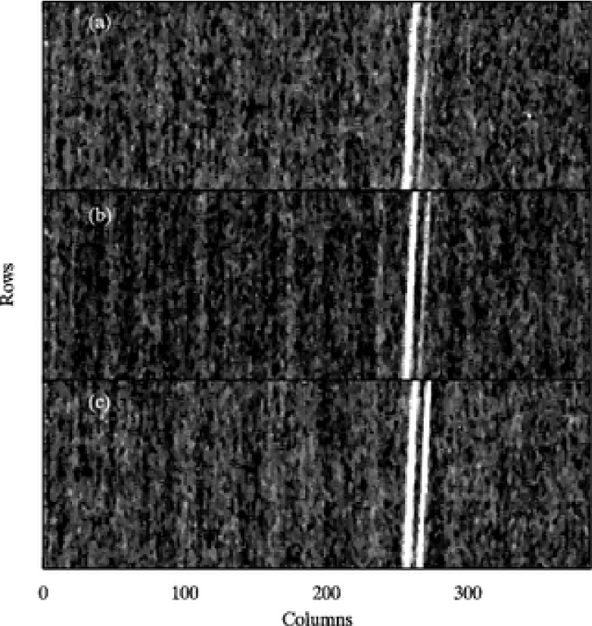
Figure 2.— Fringe variation in consecutive frames. Subsections of sky frames taken with NIRSPEC on the Keck II telescope (45 seconds integration). Fringe pattern can be seen varying between these frames (taken consecutively in order a, b, and c).

Here we present an algorithm to clean two-dimensional (2D) arrays that uses the wavelet transform, a local spectral technique (e.g., Starck & Murtagh 2002; Torrence & Compo 1998). Making use of the wavelet transform’s linearity property, the algorithm isolates the fringe pattern in wavelet space, does an inverse transform, and then obtains a clean image by subtracting the reconstructed fringe pattern. The challenge is to do this correctly in the presence of noise. The algorithm presented here is not tuned to any specific dataset and has been tested on flat field frames from ISAAC (Moorwood et al. 1998) at the Very Large Telescope (VLT) and NIRSPEC (McLean et al. 1998) at the Keck telescope.

The algorithm also provides the framework for an extension to remove fringes from object frames by interpolating the fringe pattern over spectra or point sources. Such an extension requires the design of another algorithm to interpolate fringe parameters, which is beyond the scope of the present work. Thus, our method improves the quality of extracted data when the fringes in the flat fields differ from the fringes in the data, but will not solve the problem completely if the fringes in the data array are significant. We show that there are many cases where the fringes change between arrays obtained at different times.

We implemented our algorithm in the Interactive Data Language (IDL, a product of Research Systems, Inc., Boulder, Colorado). The package (named “defringeflat”) includes tutorial documentation. It is available under the GNU General Public License from our websites or as an electronic attachment to this paper.

Section 2 gives a mathematical model of fringe formation. Section 3 describes the algorithm. Section 4 discusses performance in the presence of noise. Finally, Section 5 discusses an applied example, summarizes the benefits and limitations, and presents our conclusions.

2. FRINGES

Fringes are produced by the interference of light reflecting between parallel surfaces in an instrument. They appear in many detectors of visible and infrared light. If we ignore multiple reflections, a mathematical formulation (Rieke 2003) for the total intensity of light ($I_{a}$) received on the position $x,y$ of the detector array is given by

$$I_{a}(x,y)=I_{n}(x,y)+I_{r}(x,y)+2\sqrt{I_{n}(x,y)I_{r}(x,y)}\cos\psi(x,y),$$ (1)

where $I_{n}$ is the non-reflected intensity, $I_{r}$ is the reflected intensity, and $\psi$ is the phase difference between the two beams. We choose the $x$ coordinate such that

$$\psi(x,y)=2\pi x/P(x,y)+\xi(x,y),$$ (2)

where $P$ and $\xi$ are the period and phase of the fringe’s pattern, respectively. Let $I_{i}$ be the incoming intensity before interaction with the instrument. Then, $I_{r}(x,y)$ is proportional to the intensity incident at a nearby position:

$$I_{r}(x,y)=a(x+\delta x,y+\delta y)I_{i}(x+\delta x,y+\delta y),$$ (3)

where $\delta x$ and $\delta y$ are small displacements and the factor $a$ includes reflectivity. Note also that $a\ll 1$. If we can assume that the incoming intensity field and the reflection geometry are homogeneous on very short spatial scales, then $a(x+\delta x,y+\delta y)I_{i}(x+\delta x,y+\delta y)\approx a(x,y)I_{i}(x,y)$. On the other hand, the non-reflected intensity ($I_{n}$) is proportional to the incoming intensity ($I_{i}$) in the same coordinate, thus $I_{n}(x,y)=b(x,y)I_{i}(x,y)$. Due to energy conservation, the proportionality constant $b(x,y)$ is restricted by the previous assumption to comply with

$$a(x,y)+b(x,y)=s(x,y),$$ (4)

where $s(x,y)\lesssim 1$ accounts for losses due to scattering and absorption. Omitting the dependence on $x$ and $y$ for clarity, we find for each position

$$I_{a} = bI_{i}+aI_{i}+2I_{i}\sqrt{ab}\cos\psi$$ (5)

$$= I_{i}\left[s+2\sqrt{ab}\cos\left(2\pi x/P+\xi\right)\right]$$ (6)

$$= I_{i}\left[s+F\right],$$ (7)

where

$$F=2\sqrt{ab}\cos\left(2\pi x/P+\xi\right)$$ (8)

is the oscillating fringe term. When interacting with the detector array, Eq. 7 is modulated to obtain the detected intensity $I_{d}$. Including detection noise, the modulation is given by

$$I_{d}=I_{i}\eta\left[s+F\right]+\epsilon,$$ (9)

where $\epsilon$, which varies rapidly between pixels, includes all noise sources and $\eta$ includes quantum efficiency, and pixel collecting area, among other factors. On the other hand, $\eta$ can be decomposed as

$$\eta=\eta_{0}+\eta_{r},$$ (10)

where $\eta_{0}$ is the smoothly varying component and $\eta_{r}$ is the rapidly varying component, which includes uncorrelated differences between the sensitivities of neighboring pixels. Typically, $\eta_{r}\ll\eta_{0}$. Bringing it all together, we obtain

$$I_{d}=I_{i}\eta s+\epsilon+I_{i}\eta_{r}F+I_{i}\eta_{0}F.$$ (11)

Our algorithm makes use of the linearity property of wavelets to find and subtract the term $I_{i}\eta_{0}F$, which is the predominant contibutor at the period of the fringe pattern. The other terms will only contribute in that frequency to a background level in the amplitude of the wavelet transform. This background is considered in our algorithm (see Step II in Section 3).

Then, $\eta s$ can be corrected through flat-fielding to get the sought intensity $I_{i}$ with a modified noise $\bar{\epsilon}$ given by

$$\bar{\epsilon}=\epsilon+I_{i}\eta_{r}F.$$ (12)

With typical values, $I_{i}\eta_{r}F\ll\epsilon$.

3. ALGORITHM

The main steps in our procedure are listed in Table 1. Figs. 3 – 9 illustrate the steps of the algorithm using an example flat field. Their captions contain details regarding the example array, while the main text only refers to the algorithm in general. The example flat field is included in the defringeflat package.

Table 1Steps of Defringing Algorithm

Step	Description	Figure
	Original image with fringe	3
I	FOR EACH ROW
	$\Rightarrow$ Compute enhanced row	4
	$\Rightarrow$ Compute wavelet transform	5
II	$\Rightarrow$ FOR EACH PIXEL IN ROW
	$\Longrightarrow$ Fit fringe transform’s profile	6
III	FOR THE WHOLE ARRAY
	$\Rightarrow$ Smooth fit parameters (optional)	7
IV	FOR EACH ROW
	$\Rightarrow$ Reconstruct wavelet array	5
	$\Rightarrow$ Inverse transform	5, 8
	FOR THE WHOLE ARRAY
	$\Rightarrow$ Subtract fringe pattern to obtain clean image	9

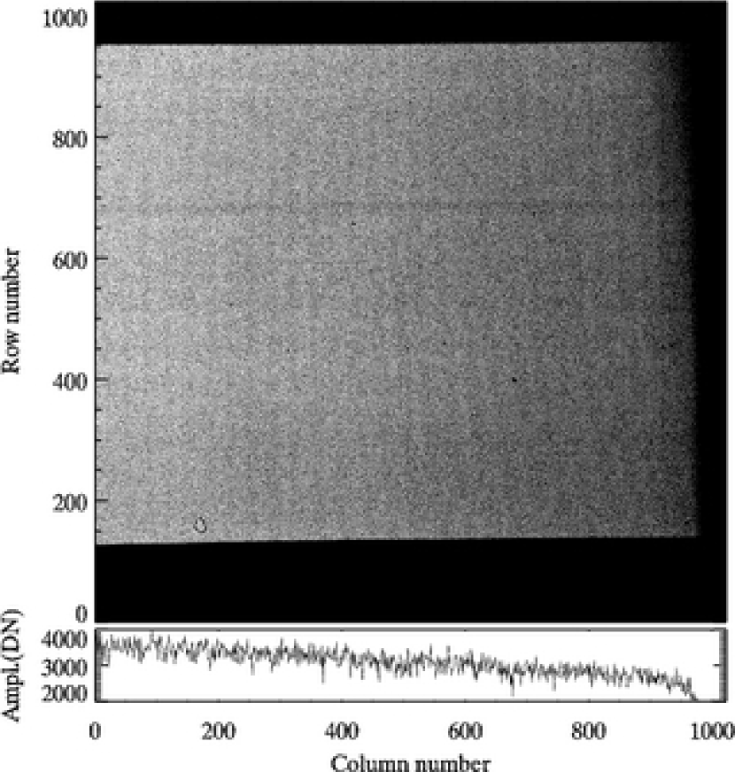
Figure 3.— Top: Sample image with fringes. This flat field was obtained with the ISAAC instrument at the VLT. Each of the numeric parameters indicated in the captions from Figs. 3 to 9 were found to be the most appropriate for this particular example, but will need to change for different images. Columns 901–1024 and rows 0–149 and 951–1024 are vignetted and thus are cropped before analysis. Periodicity can be estimated by eye at $\sim 40$ pixels in the center of the image. Bottom: Middle (512th) row.

All array borders whose values are not consistent with the image must be cropped. The fringes are allowed to have several different patterns, which do not need to look like straight lines. There are only two requirements. First, the period ($P$) of the fringe term (Eq. 8) should change smoothly accross the array; and second, only on a per-row basis, the period must be at least several pixels, but it must also have at least a few oscillations per row. To attain the second condition it is acceptable to rotate the image by 90 degrees. There are no constraints on how the phase $\xi$ can change accross rows or the range over which $P$ can vary. Hence, the algorithm can handle many patterns that do not look like plane waves, such as patterns resembling wood grain.

Step I. Enhanced Row and Wavelet Transform

For each image row we combine several surrounding rows to suppress random noise and remove bad pixels. To do this, we replace each pixel in the row with the median of a $1\times n$ sub-image centered on the pixel and traversing $n$ rows (bin width, hereafter). We then subtract a polynomial fit from the median-averaged row to obtain an enhanced row (Fig. 4). This subtraction significantly diminishes the large-period (low-frequency) oscillations of each row (and their corresponding wavelet amplitudes), allowing the next step to proceed more efficiently.

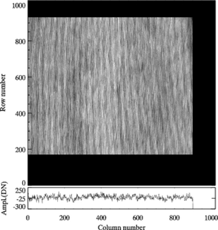
Figure 4.— Top: Enhanced rows. Each pixel of the array in Fig. 3 is first replaced by the median average of the 41 closest pixels in the vertical direction. A polynomial fit to each row is then subtracted. The fringe pattern is enhanced and some bad pixels have been removed. Note that the usable data area is reduced by 20 rows on the top and bottom because of the averaging. Bottom: Middle (512th) row.

We then compute the wavelet transform of each enhanced row. The result for each row is a two-dimensional, complex array, whose two dimensions are column number and period. There are several real and complex wavelet bases to choose from, but Step II of this algorithm requires a complex basis because real bases are not able to separate phase from amplitude information. For this particular example, we used the Morlet wavelet because its functional form is the familiar quantum-mechanical wave packet

$$\Psi(t)=\pi^{-1/4}e^{-t^{2}/2-i\omega_{0}t},$$ (13)

which makes it well suited for smoothly varying periods. Here, $t$ and $\omega_{0}$ are non-dimensional. For the Morlet basis, $\omega_{0}$ is the only parameter; it dictates the minimum number of oscillations per row. The Morlet basis also has the advantage of being compact in the frequency domain.

However, the accompanying code allows the user to choose from several other popular wavelets as they could be better suited for particular data. Steps II and III are computed over the complex array amplitudes (wavelet array, hereafter). The phases of the complex array must be stored for use in Step IV.

Step II. Parametric Fit of Fringe Transform

At the period of the fringe pattern, the wavelet array will contain a prominent fringe transform pattern traversing the columns. Its amplitude depends on the amplitude of the fringe pattern (Fig. 5). This algorithm’s success rests on our ability to distinguish this feature from the background noise level of the wavelet array. The fringe transform may vanish for particular columns, but it should be clearly distinguishable in most of each wavelet’s array. Improved sampling in period can be obtained by interpolation or by decreasing the spacing between discrete scales in the wavelet transform. A compromise should be chosen; the latter approach is more accurate but demands more computer resources.

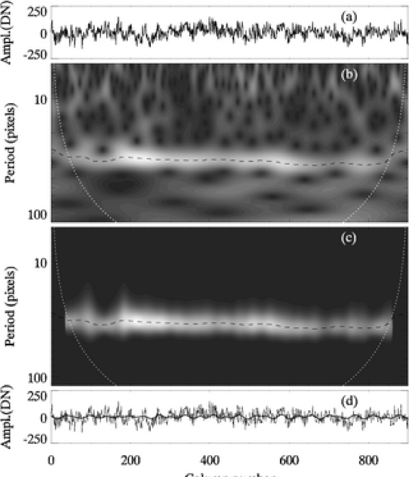
Figure 5.— Wavelet transform of an enhanced row. In the center plots, the dotted line marks the cone of influence (COI); wavelet values below this boundary should not be trusted. The dashed line shows the fitted trace. Plot a: Middle enhanced row of Fig. 4. Plot b: Amplitude of the Morlet wavelet transform of plot (a). The wavelet is interpolated in period by a spline from the period sampling of the transform, and the fringe transform, a coherent pattern corresponding to a fringe with a period of 35 pixels, is clearly visible. Plot c: Reconstructed fringe transform using a Gaussian fit (cf. Fig. 6). Plot d: Fringe pattern after applying an inverse wavelet transform to plot (c), plotted over the input data.

We next either extract or fit the fringe transform’s amplitude vs. period for a given column (Fig. 6). Starting from a reference column, the fringe profile is isolated by finding the first local minima on both sides of the reference period. Then one method is chosen to represent the profile within the minima: either we use the actual data within the minima (trueshape method, hereafter) or a parametric function can be fit to the profile. Only the latter approach will allow execution of the optional Step III. The value of the profile must be zero outside the fringe transform. Inside, on the other hand, it is recommended that the fringe transform profile exclude a background level (attributable to non-fringe image components, see discussion in Section 2). The highest point in the profile is used as the new reference period for the next column. The procedure is repeated for the whole fringe transform, extending in both directions from the reference column to the cone of influence (COI) boundary, beyond which the wavelet values are significantly contaminated by edge effects.

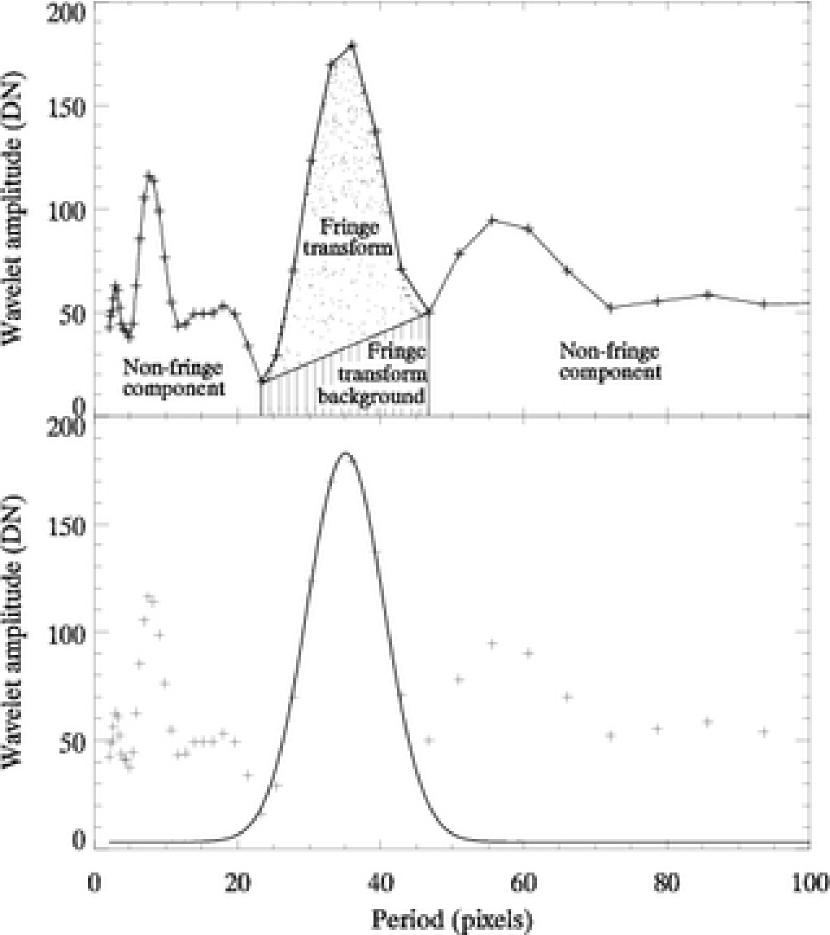
Figure 6.— Cross–section along a column of the wavelet array. Top: Components diagram. Crosses are the amplitude of the wavelet points. The data points surrounding the region labeled as “fringe transform” are exactly what the trueshape method would reconstruct or what the parametric functions will fit. The region labeled “fringe transform background” is attributable to non-fringe components; in some of the tests it was used for the wavelet reconstruction (keep) and in some it was not (nokeep). Bottom: Gaussian fit (with background) to the region between the minima. Crosses are as above, solid line is the fitted profile.

To fit the profile we have experimented with plain Gaussian fits with variable center (GVC) and Gaussian functions in which the center is fixed at the maximum height (GFC). Both Gaussian alternatives were considered without a constant background parameter (noback), and with this parameter. In the latter case, the background value can be kept or not when reconstructing (keep and nokeep, respectively). In total, we have implemented six parametric fitting methods (that can be smoothed or not in step III) and two trueshape fits (nokeep and keep), for a total of 14 fitting methods. The Gaussian shape was chosen not only because it is a natural choice to fit a peak, but also because it is the frequency-domain representation of the Morlet wavelet. The relative fringe-removal efficiency of these fits and of trueshape is discussed in Section 4.

Step III. Optional Parameter Smoothing

If a functional parametric fit was used in the previous step, one can reduce the effects of noise by forcing the reconstructed fringe’s parameters to vary smoothly. After repeating Steps I and II for every row, a 2D array is obtained for each of the fitted parameters. First, we “patch” each of the parameter arrays by finding outliers beyond a given number of standard deviations from the neighborhood median and replacing them by that median value. Then, we smooth the array with a boxcar filter. Figure 7 shows an example.

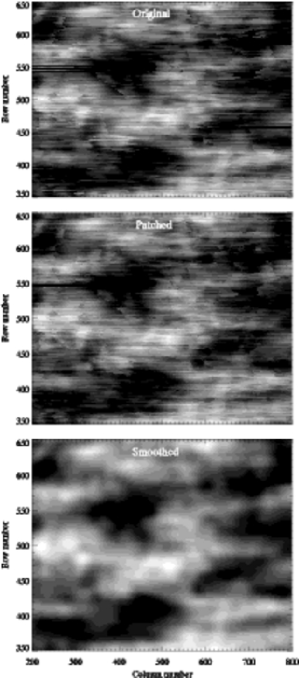
Figure 7.— Gaussian height parameter smoothing. Top: Gaussian fit height parameter for central portion of example image. Middle: Parameter after replacing all values more than $\pm 1.5\sigma$ from the local median level with that level (patched array). Bottom: Patched array after smoothing with a 19-pixel boxcar filter. This procedure is repeated for each of the other Gaussian fit parameters.

Step IV. Reconstruction of Fringe Pattern

We next evaluate the parameters to obtain the fringe’s wavelet amplitudes (Fig. 5). Far from the reconstructed fringe transform the amplitude must be zero because any non-zero value there will cause unwanted noise in the reconstructed fringe. In particular, if a keep method is chosen, the reconstructed amplitude is set to zero outside the local minima. Finally, we apply an inverse wavelet transform to the reconstructed wavelet amplitude and the corresponding complex phases (see Step I.)

We repeat these steps for every row to obtain the image’s isolated fringe pattern (Fig. 8). Due to the optional smoothing, the method to obtain the enhanced rows, and the COI boundary, the recovered fringe pattern will have smaller borders than the original image. The fringe pattern can now be subtracted from the original image (Fig. 9). Figure 10 shows another example of this algorithm for a flat field from NIRSPEC at Keck.

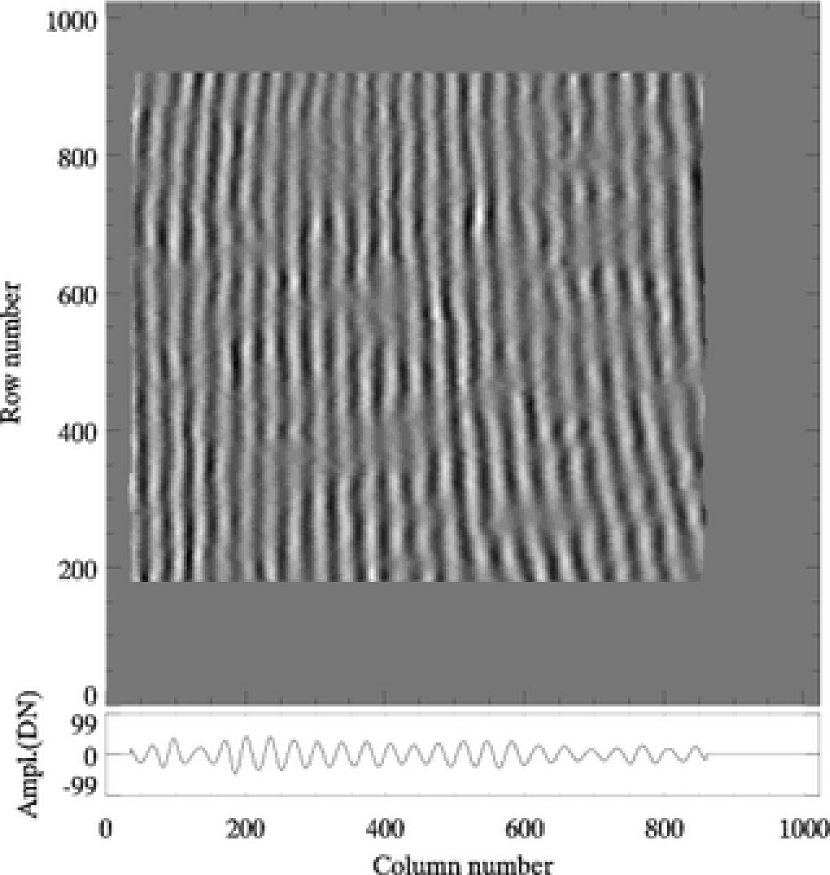
Figure 8.— Top: Reconstructed fringe pattern (cf. bottom panel of Fig. 5). Bottom: Middle (512th) row.

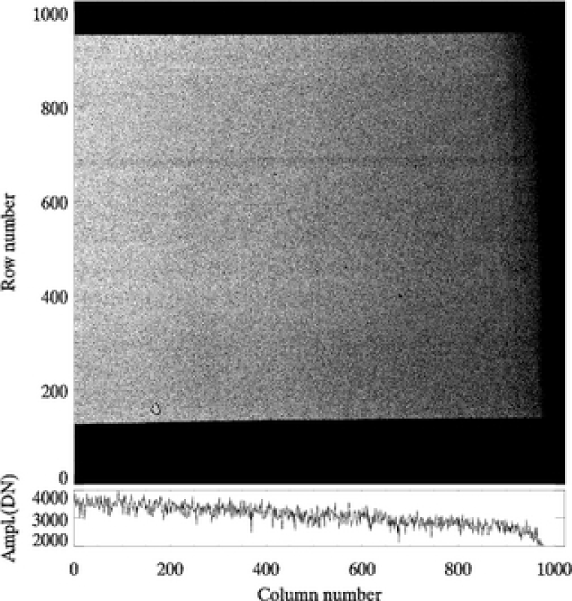
Figure 9.— Top: Cleaned image. Flat field of Fig. 3 minus the fringe pattern of Fig. 8. Note that some of the edges remain uncorrected (see text). Bottom: Middle (512th) row.

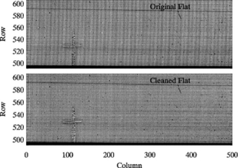
Figure 10.— Example of fringe removal from a second instrument. Frames present a portion of a debiased flat-field frame from one order of the high-resolution NIRSPEC spectrograph at the Keck II telescope. Top: Original flat field. Bottom: Same flat field defringed by our method. The algorithm had to be applied twice; once for a fringe of period $\sim 20$ pixels and then for a fringe of period $\sim 40$ pixels.

4. PERFORMANCE TESTS

The ratio of fringe pattern amplitude to the pixel-to-pixel variation (or noise) level varies among different instruments. We tested the algorithm’s performance at different noise levels by using a synthetic image consisting of a fringe pattern, a background intensity, and random noise with a Gaussian distribution that mimics pixel-to-pixel flat-field variations and photon noise.

The fringe pattern was created using an analytic function that mimics the oscillating pattern in our example image. Its functional form is

$$F(x,y)=A\sin(\nu(x,y)x+\phi(y)),$$ (14)

where $x$ and $y$ are the position indices in the array, $\phi()$ and $\nu()$ are linear functions fit to the phase and frequency, respectively, of our example’s fringe pattern, and $A$ is the amplitude. For these tests we keep the amplitude constant, but there is no reason for $A$ to be constant in a real image, nor is there any reason for a non-constant amplitude to adversely affect our algorithm. The background level is a double-linear function in both $x$ and $y$ directions and has an edge taper.

We define noise strength as the standard deviation of the Gaussian noise divided by the standard deviation of the noiseless fringe pattern ($2^{-1/2}A$, due to its sinusoidal nature). Figure 11 shows the fraction of remnant fringe after running the algorithm on simulated data with different fitting functions and varying noise strength. The remnant fringe level is not strongly dependent on noise strength and all methods show very similar behavior with slight numerical differences when the noise strength is below $\approx 8$. However, GFC consistently gives the best results in all cases, even improving when smoothing at high noise levels. Most of the methods remove over 95% of the fringe at noise strength $\approx 0.5$ and over 55% at noise strength $\approx 9$ (equivalent to Fig. 3’s noise strength). The lower plot of Fig. 11 confirms the intuitive result that the method yields better absolute results for smaller initial fringe amplitudes.

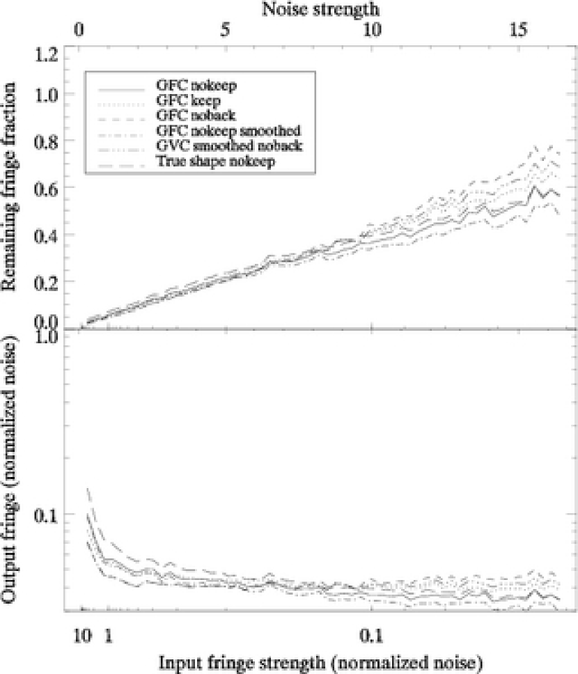
Figure 11.— Remaining fringe for varying noise strengths. Only 6 of the 14 methods are shown above, for clarity. Omitted methods are similar to plotted methods and fall within the range of traces shown. The two nokeep methods give the best results. In general, all methods give similar results for low noise strength, but smoothed nokeep methods are better for high noise strength. Top: Fraction of fringe remaining. Bottom: Absolute fringe remaining when noise level is scaled to 1.

Figure 12 shows the effect of varying the bin width. If the width is too small when computing the enhanced row, the noise is insufficiently suppressed. For low noise, a bin width that is too large will begin to average out the fringe.

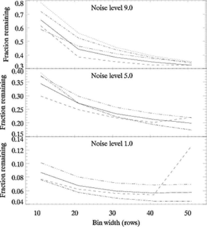
Figure 12.— Remaining fringe for different enhanced-row bin widths. The panels show the same synthetic fringe pattern as Fig. 11 at three selected noise levels. Same line styles as in Fig. 11.

The algorithm is limited by the degree to which the analytic profile fitting function mimics the data. Figure 13 shows an example of a difficult profile, which gives very different fits when using the different fitting functions. Another source of error is the potential for the algorithm to miss the correct trace in the presence of high noise in the wavelet array (Fig. 14). Also, the reconstructed fringe pattern is smaller than the input data due to the factors listed in Step IV. For the example of Fig. 3, this area is $\approx 85$% of the cropped input image, or over 90% if only considering the pixels lost for each surviving row, on average.

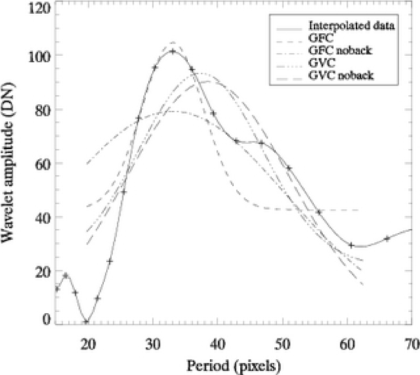
Figure 13.— Different fitting methods applied to a profile with a complicated shape. Such shapes are due to noise and are the main limiting factor for this algorithm. This profile comes from the fringe transform for row 798, column 627 of our example array. Crosses show the data points, while the solid line is the interpolated profile. Other lines are explained in the key. The profiles are only fitted within the local minima at both sides of the reference period.

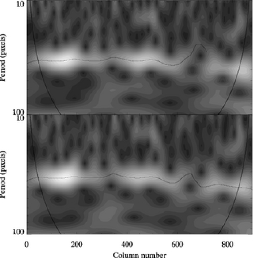
Figure 14.— Example of missed trace. Top: Wavelet array from row 798 of Fig. 4. Around column 650 the trace goes in the wrong direction, towards short period, and disappears around column 720. Bottom: Wavelet array from row 799 of Fig. 4. Array is similar to top plot but now the trace is correct through the last column. Patching in Step III is likely to correct cases like this.

5. DISCUSSION AND CONCLUSIONS

Seeking a signal from a faint source that is spatially indistinguishable from a bright source is a long-standing observational challenge. Systematic errors that would have been unimportant when analyzing only the bright source are of concern when considering the fainter source. Hence, those errors must be reduced either in the instrument design or in the data analysis. To that effect, we have developed a general algorithm to remove fringe patterns from imaging data such as flat field frames while preserving other patterns. Cleaning flat fields is especially useful when the fringe pattern varies between them and the object data.

Consider the particular example of trying to detect the spectral modulation of an extrasolar planet as it transits its star using an instrument like ISAAC at the VLT. The equivalent noise strength for a flat field of this instrument is $\approx 9$. On the other hand, no fringe was detected on the object frames up to a level equivalent to a noise strength of $\approx 1.5$. Hence, according to Fig. 11, removing the fringe in the flat fields through our method would reduce the systematic noise in the data frame by at least $40\%$. Considering the flat field intensity, this translates into residual noise in the data frame $\approx 0.25\%$ of the intensity of the star. A typical molecular spectral variation is still below that level, of order $10^{-4}$ times the stellar intensity. However, it will now be easier to use the constancy of the planetary signal over many frames to attain the required sensitivity.

There are three main limitations of this algorithm when applied to a flat field. First, the shape of a fringe in wavelet space may be much more complicated than any reasonable fitting function, resulting in a partially-corrected fringe. Second, to be able to follow the trace, the change in the fringe’s period must be smooth. Finally, there is a region along the borders where the fringe pattern cannot be recovered.

The algorithm could be improved by finding a parameter-space interpolation mechanism that would allow defringing of object frames. Also, a method could be found to fit the entire fringe transform pattern simultaneously in the 3D wavelet space of row, column, and period. The 2D wavelet transform may be more appropriate for this approach.

Our IDL implementation of this algorithm and its documentation appear as an electronic supplement to this article. Updated versions are available on our websites or by email request.

References

- Malumuth et al. (2003a) Malumuth, E. M., Hill, R. J., Cheng, E. S., Cottingham, D. A., Wen, Y., Johnson, S. D., & Hill, R. S. 2003a, in Proceedings of the SPIE., Vol. 4854, 567
- Malumuth et al. (2003b) Malumuth, E. M., Hill, R. S., Gull, T., Woodgate, B. E., Bowers, C. W., Kimble, R. A., Lindler, D., Plait, P., & Blouke, M. 2003b, PASP, 115, 218
- McLean et al. (1998) McLean, I. S., Becklin, E. E., Bendiksen, O., Brims, G., Canfield, J., Figer, D. F., Graham, J. R., Hare, J., Lacayanga, F., Larkin, J. E., Larson, S. B., Levenson, N., Magnone, N., Teplitz, H., & Wong, W. 1998, in Proc. SPIE Vol. 3354, p. 566-578, Infrared Astronomical Instrumentation, Albert M. Fowler; Ed., ed. A. M. Fowler, 566
- Mellau & Winnewisser (1995) Mellau, G. C. & Winnewisser, B. P. 1995, in ASP Conf. Ser. 81: Laboratory and Astronomical High Resolution Spectra, 138
- Moorwood et al. (1998) Moorwood, A., Cuby, J.-G., Biereichel, P., Brynnel, J., Delabre, B., Devillard, N., van Dijsseldonk, A., Finger, G., Gemperlein, H., Gilmozzi, R., Herlin, T., Huster, G., Knudstrup, J., Lidman, C., Lizon, J.-L., Mehrgan, H., Meyer, M., Nicolini, G., Petr, M., Spyromilio, J., & Stegmeier, J. 1998, The Messenger, 94, 7
- Rieke (2003) Rieke, G. H. 2003, Detection of light: from the ultraviolet to the submillimeter (Detection of light: from the ultraviolet to the submillimeter, by G.H. Rieke. 2nd ed. Cambridge, UK: Cambridge University Press, 2003)
- Starck & Murtagh (2002) Starck, J.-L. & Murtagh, F. 2002, Astronomical image and data analysis (Berlin: Springer)
- Torrence & Compo (1998) Torrence, C. & Compo, G. P. 1998, Bull. of the Am. Meteor. Soc., 79, 61