Nflation: multi-field inflationary dynamics and perturbations

Abstract

We carry out numerical investigations of the dynamics and perturbations in the Nflation model of Dimopoulos et al. (2005). This model features large numbers of scalar fields with different masses, which can cooperate to drive inflation according to the assisted inflation mechanism. We extend previous work to include random initial conditions for the scalar fields, and explore the predictions for density perturbations and the tensor-to-scalar ratio. The tensor-to-scalar ratio depends only on the number of $e$-foldings and is independent of the number of fields, their masses, and their initial conditions. It therefore always has the same value as for a single massive field. By contrast, the scalar spectral index has significant dependence on model parameters. While normally multi-field inflation models make predictions for observable quantities which depend also on the unknown field initial conditions, we find evidence of a ‘thermodynamic’ regime whereby the predicted spectral index becomes independent of initial conditions if there are enough fields. Only in parts of parameter space where the mass spectrum of the fields is extremely densely packed is the model capable of satisfying the tight observational constraints from WMAP3 observations.

I Introduction

Dimopoulos et al. DKMW have recently described an interesting addition to the collection of known inflationary models with motivation from particle theory. They consider the many axion fields predicted by string vacuum solutions, and show that these fields can work cooperatively to drive a period of inflation, via the assisted inflation mechanism LMS , without any of those fields needing to take on values in excess of the Planck scale. This ensures that the theory can be considered in the regime of radiative stability.

The prediction is that there will be large numbers of fields, all with different masses. Such a setup was first considered by Kanti and Olive KO and further explored by Kaloper and Liddle KL , in the context of Kaluza–Klein models where there would be a tower of mass eigenstates. In the axion proposal there is also a spectrum of masses states, the main difference being that these may be very closely packed. Related ideas are discussed in Ref. mfield .

Dimopoulos et al. made only a rudimentary study of the dynamics, assuming that all fields would begin with the Planck value and that all fields would slow-roll together. This leads to a prediction for density perturbations that matches that of a single massive field. Subsequently, an interesting generalization was made by Easther and McAllister EM , who used results from random matrix theory to predict the likely distribution of field masses. Their main investigation was still restricted, however, to quite specific choices of initial conditions for the fields.

Our main aim in this paper is to consider more realistic initial conditions, where each field starts in a random location within the sub-Planckian regime. We will show that this typically reduces the amount of inflation achieved, necessitating a greater number of fields. The most interesting consequence, however, concerns the perturbations that arise. Ordinarily multi-field inflation predictions depend on the initial conditions chosen (something we will verify explicitly in the two-field case) and so the models cannot be said to make definite predictions for observations, unlike the single-field case. However, focussing on the adiabatic perturbations, we find once the fields become sufficiently densely packed, the predictions once more become independent of the field initial conditions. This is essentially analogous to gas thermodynamics; once there are enough fields they probe the space of possible initial conditions well enough that the ensemble of fields can be described in a collective fashion. Even more strikingly, we find a completely model-independent prediction for the tensor-to-scalar ratio, confirming a result of Alabidi and Lyth AL .

II Multi-field dynamics and Nflation

Phenomenologically, the basic set-up of Nflation is straightforward — a set of massive uncoupled scalar fields with a particular mass spectrum. While any one of those fields is able separately to drive inflation provided it is displaced sufficiently from its minimum, if one imposes the restriction that the field value does not exceed the reduced Planck mass $M_{{\rm Pl}}$ then single-field inflation is no longer possible in such potentials. Dimopoulos et al. DKMW noted that this situation can be saved provided there are enough fields, through the assisted inflation phenomenon LMS .

Assisted inflation is simply the realization that in multi-field systems, each field feels the downward force from its own potential, but the collective frictional force from all the fields, and hence slow-roll is more easily achieved. In the original work of Liddle et al. LMS exponential potentials were studied, in which the assisted behaviour was reinforced by the presence of a late-time attractor where all fields contribute to the evolution. In the case of massive fields there is no such attractor solution, but the generic phenomenon of enhanced friction remains. With enough fields, it becomes possible to drive sufficient inflation without any field exceeding the reduced Planck mass.

For a set of uncoupled fields, the equation for the number of $e$-foldings is

$$N \simeq -\frac{1}{M_{{\rm Pl}}^{2}}\sum_{j}\int_{\phi_{j}}^{\phi_{j}^{{\rm end}}}\frac{V_{j}}{V^{\prime}_{j}}\,d\phi_{j}\,;$$ (1)

$$\simeq \frac{\sum_{j}\phi_{j}^{2}}{4M_{{\rm Pl}}^{2}}\,.$$ (2)

Here $V_{j}$ is the potential of the $j$-th field $\phi_{j}$, $V^{\prime}_{j}\equiv dV_{j}/d\phi_{j}$, and throughout there are no summations unless indicated explicitly. The last line specializes to the Nflation case of massive uncoupled fields. In this case the lower limits of the integrals, corresponding to the end of inflation, can be neglected and have been.

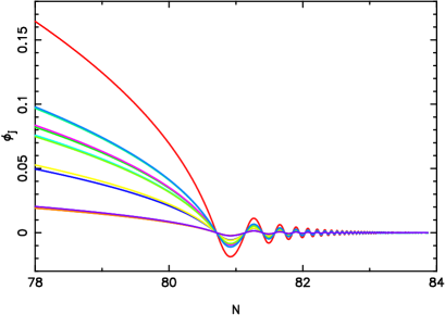
Figure 1: The evolution of eleven of the fields in a 1000-field simulation, where the field initial conditions are randomly chosen. The simulation started at $N=0$.

II.1 The equal mass case

In the very simplest case where all fields have the same mass, there is a different type of attractor corresponding to radial motion in field space. Dimopoulos et al. assumed the fields all started with the same initial condition, hence automatically placing them on this radial trajectory. With initial condition $\phi_{j}=\alpha M_{{\rm Pl}}$ they found the total number of $e$-foldings was $N_{{\rm total}}=\alpha^{2}N_{{\rm f}}/4$ where $N_{{\rm f}}$ is the total number of fields, as indeed follows immediately from Eq. (2).

We instead use random initial conditions, with the field initial conditions chosen uniformly in the range $(0,M_{{\rm Pl}})$ [which is equivalent by symmetry to $(-M_{{\rm Pl}},M_{{\rm Pl}})$]. When the fields all have the same mass they quickly adopt a radial trajectory; they all then exit the slow-roll regime simultaneously and oscillate in phase — see Fig. 1. We find that the total number of $e$-foldings achieved can be well approximated by

$$N_{{\rm total}}\simeq\frac{N_{{\rm f}}}{12}\,.$$ (3)

This indeed follows from Eq. (2) since for our initial conditions $\langle\phi_{j}^{2}\rangle=M_{{\rm Pl}}^{2}/3$. This indicates that they overestimated the number of $e$-foldings achieved by a factor of about three through not using random initial conditions. At least 600 fields are required to give the minimum acceptable amount of inflation if none of them exceeds the reduced Planck mass.

Dimopoulos et al. were also able to show that the adiabatic perturbations on this radial trajectory have the same spectral index as in the single-field case. This was subsequently confirmed in a more detailed analysis by Byrnes and Wands BW , who also noted the additional possibility of a large number of scale-invariant isocurvature perturbations from the tangential directions, which might or might not become important depending on the subsequent evolution.

II.2 A mass spectrum

For definiteness, throughout we will consider the mass spectrum suggest by Dimopoulos et al, where the fields are distributed exponentially in mass. We write the hierarchy slightly differently, normalizing to the lightest mass $m$, writing

$$m_{j}^{2}=m^{2}\exp(j/\sigma)\quad j=0,\cdots,N_{{\rm f}}-1\,.$$ (4)

Here $\sigma$ gives the density of fields per logarithmic mass interval. If one were to decide that the heaviest field should have the reduced Planck mass, as in Ref. DKMW , then that would impose a relation amongst $m$, $\sigma$ and $N_{{\rm f}}$.

Easther and McAllister EM have argued that random matrix theory predicts a somewhat different form for the mass spectrum, known as the Marc̆enko–Pastur law. Investigation of this more complicated form is beyond the scope of our present paper, and we do not expect it to lead to significant qualitative differences, but a detailed investigation would nevertheless be interesting.

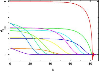
Figure 2: The evolution of eleven fields from a 1000-field simulation with different masses, with $\sigma=100$ and $N_{{\rm f}}=1000$. The fields shown are $j=0,100,\cdots,900$ and $999$. The more massive fields exit slow-roll first.

For collections of fields with different masses, within the slow-roll regime the fields obey the condition KO

$$\frac{\phi_{j}}{\phi_{j,0}}=\left(\frac{\phi_{i}}{\phi_{i,0}}\right)^{m_{j}^{2}/m_{i}^{2}}\,.$$ (5)

where $i$ is some particular index, $j$ runs over all the fields, and the subscript ‘0’ indicates initial value. This indicates that they retain a memory of their initial conditions — there is no global attractor. Further, different fields will exit slow-roll at different times; typically the high-mass fields will reach their minima first, except by chance effects of initial conditions. This has the important consequence that the dynamics of the final stages of inflation is usually determined by some number of the lightest fields in the ensemble, with the effects of any heavier fields vanishing before our observable Universe exits the horizon. Figure 2 shows a particular example.

Dimopoulos et al. did not make any detailed exploration of the dynamics in the unequal mass case, but some investigation was made by Easther and McAllister EM . They considered two choices of initial condition, by which they mean the configuration at 60 $e$-foldings before the end of inflation. The first was to take the fields to have initially the same field value, and the second to take them as having the same energy density. In either case, this ‘initial’ property is swiftly destroyed by the dynamical evolution.

We instead choose random initial conditions for the fields as described above, and compute the total number of $e$-foldings as a function of the parameters $\sigma$ and $N_{{\rm f}}$. We find that for $\sigma\gtrsim N_{{\rm f}}/10$, the amount of inflation becomes independent of $\sigma$ and is well approximated by Eq. 3 above. This confirms that of order 1000 fields are needed if all sub-Planckian. For smaller $\sigma/N_{{\rm f}}$ the fields become spread across several orders of magnitude in mass and numerical simulation becomes difficult, the expectation however being that the more massive fields fall rapidly to their minimum and play no further role before the lighter fields move significantly.

III Perturbations

We evaluate the perturbation spectrum using the formalism of Sasaki and Stewart SS , who showed that the perturbation spectrum of the curvature perturbation ${\cal R}$ at the end of inflation is given by

$${\cal P}_{\cal R}=\left(\frac{H}{2\pi}\right)^{2}\,\frac{dN}{d\phi_{i}}\,\frac{dN}{d\phi_{j}}\,\delta_{ij}\,,$$ (6)

where we follow the notation of Ref. LL , $N$ again being the number of $e$-foldings.

In general, evaluation of this expression is quite tricky, as one should compute the change in the number of $e$-foldings by tracing the trajectory past the end of inflation and through reheating until a fixed density during the radiation era. However provided the multi-field inflation adopts a straight trajectory in field space before inflation ends, the curvature perturbation will already become constant at that time. This would happen in Nflation provided the last few $e$-foldings are driven by only one field, which is likely but not inevitable.

We will approximate the formula using the slow-roll approximation, according to which it can be written LR ; EM

$${\cal P}_{\cal R} \simeq \frac{V}{12\pi^{2}M_{{\rm Pl}}^{6}}\sum_{j}\left(\frac{V_{j}}{V^{\prime}_{j}}\right)^{2}\,;$$ (7)

$$\simeq \frac{\sum_{k}m_{k}^{2}\phi_{k}^{2}}{96\pi^{2}M_{{\rm Pl}}^{6}}\sum_{j}\phi_{j}^{2}\,,$$ (8)

where $V\equiv\sum_{k}V_{k}$ is the total potential, and the second line specializes to the Nflation case. An interesting observation is that for Nflation the power spectrum is proportional to $H^{2}N$, regardless of initial conditions. In principle the summation should be only over those fields which are slowly-rolling, though we find in practice that the contribution from non-slow-rolling fields is negligible. The above expressions depend only on quantities at horizon crossing but nevertheless should offer a good approximation, as we discuss in detail below for the two-field case.

The spectral index is then given by SS

$$n_{{\rm S}}-1 \simeq -\frac{M_{\rm Pl}^{2}}{V^{2}}\sum_{k}(V^{\prime}_{k})^{2}-\frac{2M_{\rm Pl}^{2}}{\sum_{j}\left(V_{j}/V^{\prime}_{j}\right)^{2}}$$ (9)

$$+\frac{2M_{\rm Pl}^{2}}{V}\left[\frac{\sum_{l}\left({V_{l}}/{V^{\prime}_{l}}\right)^{2}V^{\prime\prime}_{l}}{\sum_{j}\left({V_{j}}/{V^{\prime}_{j}}\right)^{2}}\right]\,;$$

$$\simeq -4M_{\rm Pl}^{2}\left[\frac{\sum_{k}m_{k}^{4}\phi_{k}^{2}}{(\sum_{l}m_{l}^{2}\phi_{l}^{2})^{2}}+\frac{1}{\sum_{j}\phi_{j}^{2}}\right]\,,$$ (10)

where again the last line specializes to Nflation.

The other main inflationary observable is the tensor-to-scalar ratio $r$. The tensor spectrum is given by the usual formula, as it depends only on the expansion rate history $H(a)$,

$${\cal P}_{g}=\frac{2H^{2}}{\pi^{2}M^{2}_{\rm Pl}}\simeq\frac{2V}{3\pi^{2}M_{\rm Pl}^{4}}\,.$$ (11)

Thus the tensor-to-scalar ratio is given by

$$r\cong\frac{{\cal P}_{g}}{{\cal P}_{\cal R}} \simeq \frac{8M_{\rm Pl}^{2}}{\sum_{j}\left({V_{j}}/{V^{\prime}_{j}}\right)^{2}}\,;$$ (12)

$$\simeq \frac{32M^{2}_{\rm Pl}}{\sum_{j}\phi_{j}^{2}}\simeq\frac{8}{N}\,,$$ (13)

with the last line holding only for the Nflation case of massive coupled fields and which uses Eq. (2).

This last formula immediately gives a striking result first noted by Alabidi and Lyth AL : in Nflation the tensor-to-scalar ratio is independent (within the slow-roll approximation) of the number of fields present, their masses, and their initial conditions. It is given simply by the number of $e$-foldings at which the expression is evaluated. This result is confirmed by our numerical code, with variation only in the third significant figure due to slow-roll corrections. Nflation therefore gives a definitive prediction for the tensor-to-scalar ratio, and moreover one that is readily accessible to upcoming experiments.

We will throughout assume that the observable scales crossed outside the horizon 50 $e$-foldings before the end of inflation. For comparison with later results, the observables obtained for a single massive field are given by

$$n_{{\rm S}}-1 = -0.04\quad(-0.0404)$$ (14)

$$r = 0.16\quad\;\;\>(0.162)$$ (15)

where the first number uses the slow-roll approximation both for the spectrum and for computing the 50 $e$-foldings point, and the number in brackets shows how this is corrected if the 50 $e$-foldings point is computed numerically (as is the case for the multi-field results we will display). The observed normalization of the spectrum can be taken as ${\cal P}_{\cal R}^{1/2}=5\times 10^{-5}$ LL , leading to a normalization of

$$\frac{m}{M_{{\rm Pl}}}=7.8\times 10^{-6}\,,$$ (16)

in the single-field case.

III.1 The two-field case

As a test of our code, we first study the case of two massive fields. This was previously studied in the slow-roll approximation by Lyth and Riotto LR , and more recently using full trajectory integration by Vernizzi and Wands VW .

Starting with the Lyth–Riotto result, they used the slow-roll approximation for both fields and found that the spectral index was given by

$$n_{\rm S}-1 \simeq -\frac{1}{N}\left[1+\frac{(1+f)(1+R^{4}f)}{(1+R^{2}f)^{2}}\right]\,;$$ (17)

$$= -\frac{1}{N}\left[2+\frac{(R^{2}-1)^{2}f}{(1+R^{2}f)^{2}}\right]\,,$$

where $f\equiv\phi_{2}^{2}/\phi_{1}^{2}$ and $R\equiv m_{2}/m_{1}$. This is indeed the two-field version of Eq. (10), using Eq. (2). The prediction depends explicitly on $f$, which is the ratio of the values of the two fields at 50 $e$-foldings, showing clearly that this model makes no unique prediction for the spectral index.

This expression has various symmetries. For instance, the spectral index is independent of $f$ in the equal-mass case and takes on the single-field value. It is of course invariant under simultaneous interchange $R\rightarrow 1/R$ and $f\rightarrow 1/f$, corresponding to swapping the labels on the fields. The general form of the correction to the single-field result is however quite complex, with it becoming large in some parts of the $R$–$f$ plane.

A more sophisticated treatment of the two-field model was recently given by Vernizzi and Wands VW , who provide a formalism able to track the evolution of the spectral amplitude and index during inflation up until its final value. Their expression for the spectral index mostly features terms evaluated at horizon crossing, plus one additional term denoted $Z_{c}$. This term accounts for the contribution to the change in $e$-foldings at the final uniform-density hypersurface, and evolves during inflation driving evolution of $n_{{\rm S}}$. If $Z_{c}$ is set to zero, our formula Eq. (10) is recovered. We have reproduced their calculation, and find that while $Z_{c}$ is substantial at horizon crossing, it becomes negligible by the end of inflation. Accordingly, our expression is an excellent approximation to the desired answer, being the one at the end of inflation, even though it is entirely evaluated at horizon crossing.

This convergence relies on all but one of the fields becoming dynamically unimportant before inflation ends, which may be true of typical trajectories but cannot be absolutely generic. In principle one should then solve the problem numerically, but unfortunately this is not tractable for the large number of fields that we are considering (as one has to solve a trajectory for a separate perturbation in each field direction), and so we adopt the slow-roll formula.

There is also the question of whether further perturbations might be generated after inflation, for instance by a curvaton-like mechanism (see e.g. the discussion in Ref. VW ). Such effects would be absent if the late stages of inflation are driven by a single field, but otherwise would depend on the routes by which the scalar fields decay into conventional and dark matter. We assume such effects are absent.

III.2 Nflation perturbations: amplitude

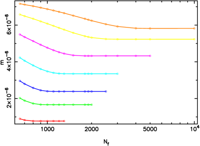
Figure 3: The mass $m$ of the lightest field, determined from the normalization of the power spectrum. This is shown as a function of the number of fields $N_{{\rm f}}$ for a range of values of $\sigma$ (from bottom to top, $\sigma=100$, $150$, $200$, $300$, $500$, $1000$ and $2000$).

We first investigate the normalization of the mass spectrum enforced by the perturbation amplitude. This is shown in Fig. 3 for a set of values of $\sigma$. The single-field normalization is attained in the limit $N_{{\rm F}}\ll\sigma$, in which the field packing becomes very close and the equal mass case is attained, though only the highest line shown here comes close to that case.

For a given value of $\sigma$, each curve flattens once $N_{{\rm f}}\gg\sigma$. This indicates that the most massive fields are no longer playing a role during the last 50 $e$-foldings of inflation, having fallen to their minima before observable scales leave the horizon. This flattening is a generic property of all observables.

III.3 Nflation perturbations: spectral index

The most important observable is the spectral index, which we calculate as described above and show in Fig. 4. Each point is the average value obtained over ten simulations with different random initial conditions. As with all observables, the single-field value is attained in the limit $N_{{\rm f}}\ll\sigma$, in which we reproduce the result of Byrnes and Wands BW that the perturbations match the single-field form. But otherwise significant differences are seen, which in some cases is enough to put the model outside the region permitted by the WMAP3 data wmap3 .

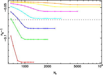
Figure 4: The predicted average value of the spectral index as a function of the number of fields $N_{{\rm f}}$, shown for a range of values of $\sigma$ (from bottom to top, $\sigma=100$, $150$, $200$, $300$, $500$, $1000$ and $2000$). The left-hand edge of the graph roughly corresponds to the minimum number of fields needed to achieve sufficient inflation, and the dotted line shows the observational lower limit on $n_{{\rm S}}$ from WMAP3.

Again we see the flattening of the curves for sufficiently large $N_{{\rm f}}$, indicating that the most massive fields play no dynamical role in the last 50 $e$-foldings.

The results shown in Fig. 4 are the mean values over realizations of the initial conditions. However we also find that the spread in $n_{{\rm S}}$ values is quite small; the standard deviation of $n_{{\rm S}}$ is never more than a few percent of its displacement from unity for all the values shown in that graph. The scatter in the mass normalization shown in Fig. 3 is also at the few percent level at most. We conclude that with such large numbers of fields, the observational predictions are to a good approximation independent of the field initial conditions. The mass spectrum is sufficiently dense that the space of initial conditions is well explored in each realization, and a well-defined prediction for $n_{{\rm S}}$ emerges in a manner analogous to the emergence of macroscopic thermodynamic quantities.

We are now in a position to discuss what is permitted by observations, using WMAP3 constraints in the inflationary $n_{{\rm S}}$–$r$ plane wmap3 . We use limits obtained from WMAP3 data alone. All models predict $r\simeq 0.16$, for which value the 95% range on $n_{{\rm S}}$ is $0.93\leq n_{{\rm S}}\leq$1.02, only the lower limit interesting us.

We see in Fig. 4 that this is a significant constraint which is failed in large parts of parameter space. Provided $\sigma$ exceeds about 280, the spectral index is always large enough regardless of the number of fields, provided that the lower limit $N_{{\rm f}}\gtrsim 600$ to obtain sufficient inflation is exceeded. As $\sigma$ reduces, an upper limit is then placed on the number of fields. This limit rapidly comes into contradiction with the sufficient $e$-foldings condition, so that by $\sigma=150$ there are almost no viable models at all (this result presumes that no field value exceeds the Planck mass). We conclude that Nflation is observationally viable only if the fields are both numerous and very densely packed.

IV Conclusions

We have carried out a detailed investigation of the inflationary dynamics and perturbations in Nflation models. The tensor-to-scalar ratio is completely independent of the model parameters, i.e. the number of fields and their mass spectrum, and also independent of the field initial conditions. Nflation therefore makes the definitive prediction that $r=8/N$ AL , where $N$ is the number of $e$-foldings corresponding to when the comoving wavenumber at our present Hubble radius equalled the Hubble radius during inflation (typically $N\simeq 50$). That there is a unique prediction is a feature only of the case of uncoupled fields with polynomial potentials piao . This prediction is readily testable by upcoming experiments.

The spectral index, by contrast, is dependent on both the number of fields, $N_{{\rm f}}$, and the density of fields in the mass spectrum, $\sigma$. Provided $\sigma$ is large enough, it is however independent of the initial conditions as they are statistically explored sufficiently well by the densely-packed fields. This is analogous to the emergence of macroscopic quantities in thermodynamics. For any given $\sigma$, results also become independent of the number of fields once it is large enough, as the most massive ones fall into their minima before observable scales cross outside the horizon.

In terms of observations, if the density of fields is large enough, $\sigma\gtrsim 280$, then a satisfactory spectral index is always achieved regardless of the number of fields, provided this number exceeds the minimum of around 600 needed to give sufficient inflation. For smaller $\sigma$, compatibility with observations imposes an upper limit on the number of fields, which rapidly becomes incompatible with the condition for sufficient inflation, giving a minimum $\sigma$ of 150 to have a successful scenario. Observations therefore require the Nflation model both to have a large number of fields and for these fields to have a very densely packed mass spectrum.

- (1) S. Dimopoulos, S. Kachru, J. McGreevy, and J. Wacker, hep-th/0507205.
- (2) A. R. Liddle, A. Mazumdar, and F. E. Schunck, Phys. Rev. D58, 061301(R) (1998), astro-ph/9804177.
- (3) P. Kanti and K. A. Olive, Phys. Rev. D60, 043502 (1999), hep-ph/9903524; P. Kanti and K. A. Olive, Phys. Lett. B464, 192 (1999), hep-ph/9906331.
- (4) N. Kaloper and A. R. Liddle, Phys. Rev. D61, 123513, (2000), hep-ph/9910499.
- (5) A. Jokinen and A. Mazumdar, Phys. Lett. B597, 222 (2004), hep-th/0406074; K. Becker, M. Becker, and A. Krause, Nucl. Phys. B715, 349 (2005), hep-th/0501130.
- (6) R. Easther and L. McAllister, JCAP 0605, 018 (2006), hep-th/0512102.
- (7) L. Alabidi and D. H. Lyth, JCAP 0605, 016 (2006), astro-ph/0510441
- (8) C. T. Byrnes and D. Wands, Phys. Rev. D73, 063509 (2006), astro-ph/0512195.
- (9) M. Sasaki and E. D. Stewart, Prog. Theor. Phys. 95, 71 (1996), astro-ph/9507001.
- (10) A. R. Liddle and D. H. Lyth, Cosmological inflation and large-scale structure, Cambridge University Press, Cambridge (2000).
- (11) D. H. Lyth and A. Riotto, Phys. Rep. 314, 1 (1999), hep-ph/9807278.
- (12) F. Vernizzi and D. Wands, JCAP 0605, 019 (2006), astro-ph/0603799.
- (13) S. Yokoyama, T. Tanaka, M. Sasaki, and E. D. Stewart, astro-ph/0605021.
- (14) D. N. Spergel et al. (WMAP Collaboration), astro-ph/0603449; G. Hinshaw et al. (WMAP Collaboration), astro-ph/0603451; L. Page et al. (WMAP Collaboration), astro-ph/0603450.
- (15) W. Kinney, E. W. Kolb, A. Melchiorri, and A. Riotto, astro-ph/0605338.
- (16) Y.-S. Piao, gr-qc/0606034.