Constraints on holographic dark energy models using the differential ages of passively evolving galaxies

Abstract

Using the absolute ages of passively evolving galaxies observed at different redshifts, one can obtain the differential ages, the derivative of redshift $z$ with respect to the cosmic time $t$ (i.e. ${\rm d}z/{\rm d}t$). Thus, the Hubble parameter $H(z)$ can be measured through the relation $H(z)=-({\rm d}z/{\rm d}t)/(1+z)$. By comparing the measured Hubble parameter at different redshifts with the theoretical one containing free cosmological parameters, one can constrain current cosmological models. In this paper, we use this method to present the constraint on a spatially flat Friedmann-Robert-Walker Universe with a matter component and a holographic dark energy component, in which the parameter $c$ plays a significant role in this dark energy model. Firstly we consider three fixed values of $c$=0.6, 1.0 and 1.4 in the fitting of data. If we set $c$ free, the best fitting values are $c=0.26$, $\Omega_{\rm m0}=0.16$, $h=0.9998$. It is shown that the holographic dark energy behaves like a quintom-type at the $1\sigma$ level. This result is consistent with some other independent cosmological constrains, which imply that $c<1.0$ is favored. We also test the results derived from the differential ages using another independent method based on the lookback time to galaxy clusters and the age of the universe. It shows that our results are reliable.

Keywords: Cosmology; cosmological parameters; holographic dark energy; the differential ages of galaxies

PACS numbers: 98.80.-k, 98.80.Es, 98.80.Cq, 95.35.+d

1 Introduction

The type Ia Supernova (SN Ia) observations indicate that the expansion of our Universe is accelerating today [1,2], which can be explained by an exotic component, referred to as dark energy, with a large negative pressure. The most obvious candidate of dark energy is the cosmological constant [3]. In addition, many other cosmological models such as the quintessence [4], the Chaplygin Gas [5], the braneworld models [6], the Cardassian models [7] are proposed to explain the accelerating expansion of the Universe. Recently, Cohen et al. [8] suggested the holographic dark energy model to reconcile the breakdown in quantum field theory caused by the conflict between the effective field theory and the so-called Bekenstein entropy bound [9,10]. For an effective field theory, in a box of size $L$ with UV cut-off $\Lambda$, the entropy $S$ scales extensively, $S\sim L^{3}\Lambda^{3}$. But for the Bekenstein entropy bound, $S$ is non-extensive, $S\leq S_{\rm BH}\equiv L^{2}/8G$. This is postulated from the peculiar thermodynamics of a black hole. Cohen et al. also pointed out that, if the zero-point energy density $\rho_{\rm H}$ is related to a UV cut-off, the total energy of the whole system with size $L$ should not exceed a black hole of the same size, i.e. $\rho_{\rm H}\leq L^{-2}/8\pi G$. It means that the maximum entropy is in order of $S_{\rm BH}^{3/4}$. A short distance UV cut-off and a long distance IR cut-off have been connected together. If we apply this to the Universe, the vacuum energy related to the holographic principle [11] is called the holographic dark energy. Thus the holographic dark energy density $\rho_{\rm H}$ is written as

$$\rho_{\rm H}=\frac{3c^{2}}{8\pi G}L^{-2},$$ (1)

where $c$ is a numerical constant. As proposed by Li [12], we take the scale $L$ as the size of the future event horizon

$$R_{\rm h}(a)=a\int_{t}^{\infty}\frac{{\rm d}t}{a(t)}=a\int_{a}^{\infty}\frac{{\rm d}a^{\prime}}{Ha^{\prime 2}},$$ (2)

where $a$ is the scale factor of the Universe, $t$ is the cosmic time and $H$ is the Hubble parameter. Such a dark energy model has been constrained through many kinds of astronomical observations, including SN Ia [13], X-ray gas mass fraction of galaxy clusters [14] and a joint analysis of SN Ia and CMB and LSS observational data [15].

It is noted that $c$ is one key parameter in the holographic dark energy model [13-15], which determines the evolutionary behavior of the space-time and the ultimate fate of the Universe. Huang et al. [13] suggested $c=0.21$ through a direct fit to the present available SN Ia data. Zhang et al. [15] showed $c=0.81$ by combining SN Ia and CMB and LSS. Kao et al. [16] showed that the reasonable result is $c\sim 0.7$ by calculating the average equation of state and the angular scale of the oscillation from the BOOMERANG and WMAP data on the CMB observation.

Unlike the observational data mentioned above, Simon et al. [17] used the relative ages of a sample of passively evolving galaxies and supernova data to reconstruct the potential of dark energy. They showed that the reconstructed potentials from galaxy ages and SN are consistent. In this paper, we attempt to apply the differential ages of galaxies [17,18] to the constraint on the holographic dark energy model. If we take some fixed values $c$=0.6, 1.0 and 1.4, the corresponding results of $h$ and $\Omega_{\rm m0}$ are not too far from each other. If we set all the parameters free, the best fitting result is $\Omega_{\rm m0}=0.16$, $h=0.9998$, $c=0.26$, corresponding to a quintom-type dark energy at the $1\sigma$ level. This result is consistent with some other independent cosmological tests. In addition, we attempt to test the fitting results using another independent method based on the data for the lookback time to galaxy clusters [19] and the age of the universe. It is shown that our method is acceptable.

This paper is organized as follows. In Sec.2, we briefly review the holographic dark energy model. Differential ages of galaxies and constraints on holographic dark energy model are presented in Sec.3, while another independent method based on the lookback time to galaxy clusters and the age of the universe is used to test our conclusions in Sec.4. The deceleration parameter $q$ and equation of state $\omega$ are discussed in in Sec.5. Conclusions and discussions are given in the last section.

2 The Holographic Dark Energy Model

Recent observations indicate that our Universe has a flat geometry [20]. Here we consider a spatially flat Friedmann-Robert-Walker Universe with a matter component $\rho_{\rm m}$ (including both baryon mater and cold dark matter) and a holographic dark energy component $\rho_{\rm H}$, which means $\Omega_{\rm m}+\Omega_{\rm H}=1$. Therefore, the Friedman equation reads

$$\frac{3H^{2}}{8\pi G}=\rho_{\rm m}+\rho_{\rm H},$$ (3)

or taking this form equivalently

$$\frac{H^{2}}{H_{\rm 0}^{2}}=\Omega_{\rm m0}a^{-3}+\Omega_{\rm H}\frac{H^{2}}{H_{\rm 0}^{2}},$$ (4)

where $\Omega_{\rm m0}=\rho_{\rm m0}/\rho_{\rm c}$, $\Omega_{\rm H}=\rho_{\rm H}/\rho_{\rm c}$, $\rho_{\rm c}=3H_{\rm 0}^{2}/8\pi G$ and $H_{\rm 0}=100h$ km s^-1 Mpc^-1 is the Hubble constant. Combining Eq.(1) and Eq.(2), we derive

$$\int_{a}^{\infty}\frac{d{\rm ln}a^{\prime}}{Ha^{\prime}}=\frac{c}{Ha\sqrt{\Omega_{\rm H}}}.$$ (5)

Meanwhile we notice that Eq.(4) can be deduced to

$$\frac{1}{Ha}=\sqrt{a(1-\Omega_{\rm H})}\frac{1}{H_{\rm 0}\sqrt{\Omega_{\rm m0}}}.$$ (6)

Substituting Eq.(6) into Eq.(5) and taking derivative with respect to ln$a$ on both sides, we get

$$\frac{d\Omega_{\rm H}}{d{\rm ln}a}=\Omega_{\rm H}(1-\Omega_{\rm H})(1+\frac{2}{c}\sqrt{\Omega_{\rm H}}),$$ (7)

which describes the dark energy’s evolution along with the factor ln$a$ completely. And it can also be solved analytically as follows

$${\rm ln}\Omega_{\rm H}-\frac{c}{2+c}{\rm ln}(1-\sqrt{\Omega_{\rm H}})+\frac{c}{2-c}{\rm ln}(1+\sqrt{\Omega_{\rm H}})-\frac{8}{4-c^{2}}{\rm ln}(c+2\sqrt{\Omega_{\rm H}})=-{\rm ln}(1+z)+y_{0},$$ (8)

where $y_{0}$ can be determined by given $\Omega_{\rm H0}$ and $c$. From Eq.(4), it is easy to get the theoretical Hubble parameter

$$H(z)=H_{0}\sqrt{\frac{\Omega_{\rm m0}(1+z)^{3}}{1-\Omega_{\rm H}}},$$ (9)

where $\Omega_{\rm H}$ is a function of $\Omega_{\rm H0}$ and $c$, i.e., $\Omega_{\rm H}=f(\Omega_{\rm H0},c)$ and $\Omega_{\rm m0}+\Omega_{\rm H0}=1$.

3 Differential Ages of Galaxies and Constraints on Holographic Dark Energy

The Hubble parameter depends on the differential age of the Universe as a function of $z$ in this form

$$H(z)=-\frac{1}{1+z}\frac{{\rm d}z}{{\rm d}t},$$ (10)

so $H(z)$ can be directly measured through a determination of ${\rm d}z/{\rm d}t$. By comparing the measured Hubble parameter at different redshifts with the theoretical one containing some free cosmological parameters, we can constrain current cosmological models.

In this paper, we adopt data from [17] where the new publicly released Gemini Deep Survey (GDDS) survey [21] and archival data [22-26] were used to infer $dz/dt$ and the shape as well as redshift dependence of dark energy potential were constrained. The data contain the absolute ages of 32 passively evolving galaxies, which are further divided into three subsamples. The first subsample was composed of 10 field early-type galaxies, after discarding galaxies for which the spectral fit indicated an extended star formation. The ages of this sample were derived using the SPEED models [27]. The second subsample was composed of 20 old passive galaxies from GDDS. The GDDS old sample was reanalyzed using SPEED models and the ages of this sample were obtained within 0.1Gyr of the GDDS collaboration estimate. The third subsample consisted of two reddest radio galaxies 53W091 and 53W069 in the survey of Windhorst et al. [24-26]. Then 8 numerical values of differential ages $dz/dt$, equivalently $H(z)$, were obtained. The detailed procedure on calculating the differential ages can be found in [17].

The parameters of the holographic dark energy model can be determined by minimizing

$$\chi^{2}=\sum_{i}\frac{[H_{\rm th}(z_{i})-H_{\rm de}(z_{i})]^{2}}{\sigma_{i}^{2}},$$ (11)

where $H_{\rm th}(z_{i})$ is the theoretical Hubble parameter as Eq.(9), $H_{\rm de}(z_{i})$ is the Hubble parameter derived from the differential ages as Eq.(10) and $\sigma_{i}$ is the corresponding $1\sigma$ error bar. All the fitting results are listed in Table.1 for the fixed choice of $c$=0.6, 1.0 and 1.4. We can see that the result of $c=0.6$ is roughly consistent with Chang et al: $c=0.61$, $\Omega_{\rm m0}=0.24$, $h=0.73$ by X-ray gas mass fraction of galaxy clusters [14]. For the case of $c=1.0$, Huang & Gong [13] suggested $\Omega_{\rm m0}=0.25_{-0.03}^{+0.04}$ using 157 gold sample in [28] and $\Omega_{\rm m0}=0.25\pm 0.03$ using 186 gold and silver SN sample. If $c$ is set to be free, the best fitting result is $c=0.26\pm 0.37$, $\Omega_{\rm m0}=0.16\pm 0.20$, $h=0.9998\pm 0.6903$ and $\chi_{\rm min}^{2}=7.61$. The best fitting value of $\Omega_{\rm m0}$ is quite smaller and $h$ is quite larger than the result of WMAP [29]. The fitting value of $c$ is roughly consistent with $c=0.21$ in [13] although the value of $\Omega_{\rm m0}$ is smaller than $\Omega_{\rm m0}=0.46$ there. But Zhang et al. [15] showed $c=0.81$, $\Omega_{\rm m0}=0.28$, $h=0.65$ by combining SN Ia data and the CMB and LSS data. We plot $H$ as a function of $z$ in Fig.1 using the best fitting values.

Table 1: The fitting results for the fixed cases: $c$=0.6, 1.0 and 1.4.

	$c=0.6$	$c=1.0$	$c=1.4$
$\Omega_{\rm m0}$	$0.24\pm 0.08$	$0.23\pm 0.08$	$0.21\pm 0.09$
$h$	$0.78\pm 0.09$	$0.74\pm 0.08$	$0.71\pm 0.07$
$\chi_{\rm min}^{2}$	$7.62$	$7.61$	$7.59$

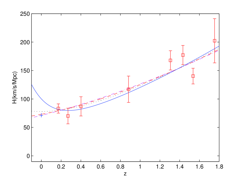
Figure 1: $H$ as a function of $z$ for the holographic dark energy models. The dot line corresponds to $c=0.6$, $\Omega_{\rm m0}=0.24$, $h=0.78$, the dash $c=1.0$, $\Omega_{\rm m0}=0.23$, $h=0.74$ and the dash-dot $c=1.4$, $\Omega_{\rm m0}=0.21$, $h=0.71$. The solid line represents the case of considering $c$ free, $c=0.26$, $\Omega_{\rm m0}=0.16$ and $h=0.9998$. The open squares with $1\sigma$ error bar are the derived values from the differential ages of galaxies, while the plus symbol stands for the result of WMAP $h=0.71_{-0.03}^{+0.04}$ [29].

The confidence regions in the $\Omega_{\rm m0}-h$ plane are plotted in Fig.2 for $c$=0.6, 1.0 and 1.4 respectively. We can see that $\Omega_{\rm m0}$ and $h$ are constrained a little poorly. The confidence regions in the $\Omega_{\rm m0}-c$ plane for setting $c$ free, after marginalizing the likelihood function over $h$, are plotted in Fig.3. And what we have to point out is that we’ve assumed an approximate Gaussian prior for a convenience during this work. The contour plots show $c\lesssim 0.81$ at the $1\sigma$ level although we can not exclude the existence of $c>1.0$ at $95.4\%$ confidence level. This is in good agreement with some other independent cosmological constraints [13,14].

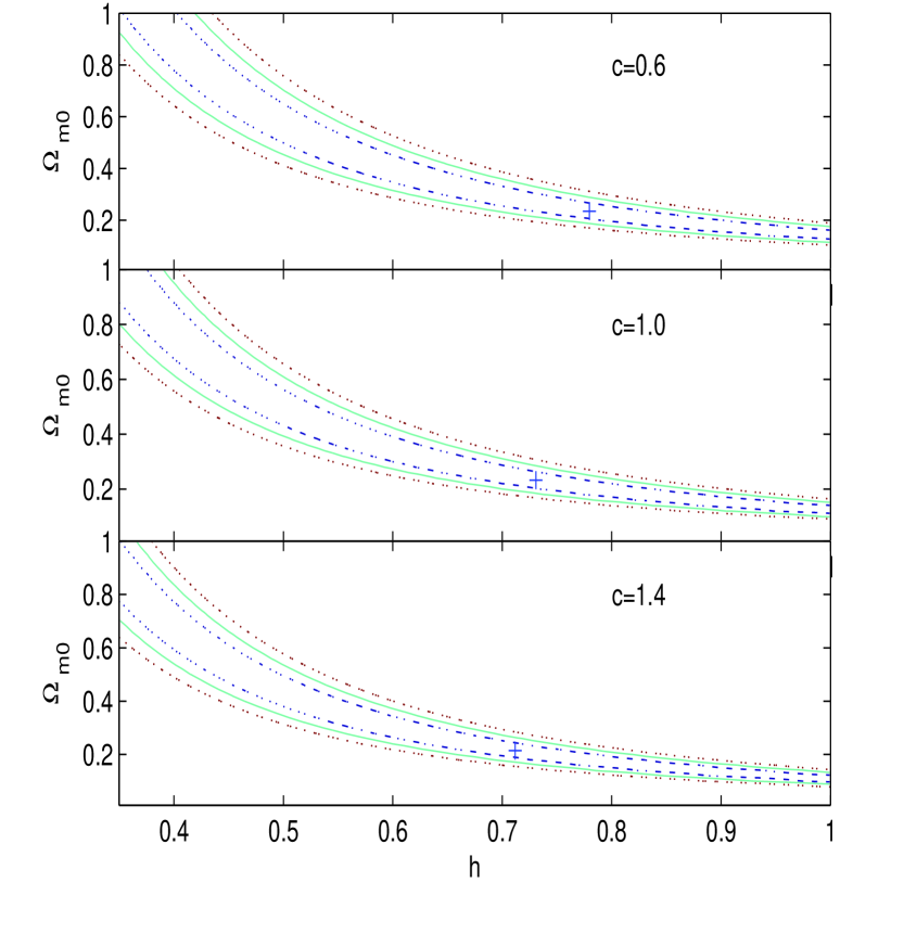
Figure 2: Confidence regions in the $\Omega_{\rm m0}-h$ plane for $c=$0.6, 1.0 and 1.4. The dash-dot line corresponds to the confidence level of 68.3%, the solid 95.4% and the dash 99.7% respectively. The cross stands for the respective best fitting values.

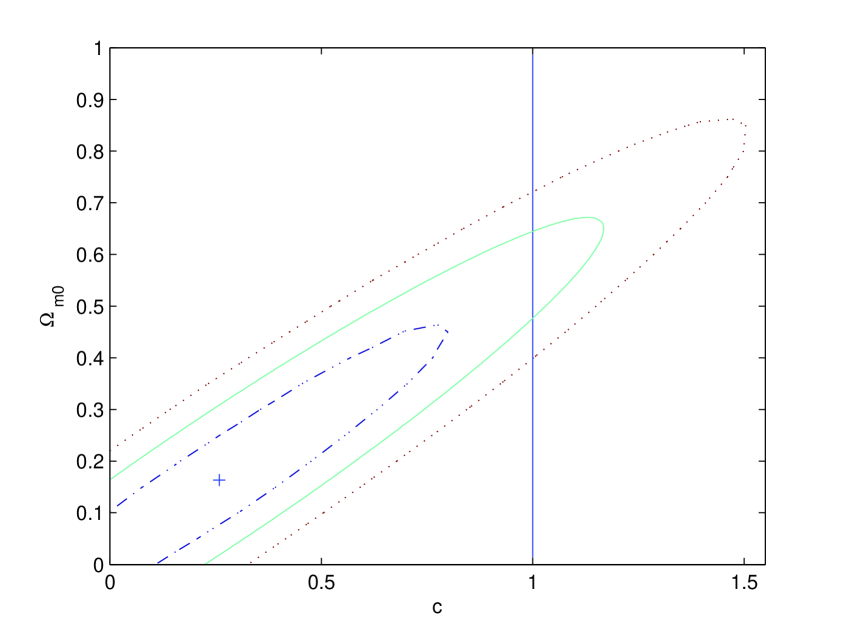
Figure 3: Same as Fig.2, but in the $\Omega_{\rm m0}-c$ plane marginalizing the likelihood function over $h$ and setting $c$ free.

4 An Independent Constraints Using the Lookback Time to Galaxy Clusters and the Age of the Universe

In order to guarantee the reliability of the method above, we make a further independent constraint on the model using the lookback time to galaxy clusters [19] and the age of the universe [30]. Dalal et al. [31] proposed the use of the lookback time to high redshift objects to constrain cosmological models. Capozziello et al. [19] constrained the quintessence model, the parametric density model and the curvature quintessence model using the lookback time to galaxy clusters and the age of the universe.

Following the reference [19], the lookback time $t_{\rm L}$ can be defined as the difference between the age of the universe at present and the age at redshift $z$

$$t_{\rm L}(z;\textbf{P})=\int_{0}^{z}\frac{dz^{\prime}}{(1+z^{\prime})H(z^{\prime};\textbf{P})},$$ (12)

where P is a set of parameters characterizing a given cosmological model and $H(z^{\prime};\textbf{P})$ is the corresponding theoretical Hubble parameter. For the holographic dark energy model, $\textbf{P}=(H_{0},\Omega_{\rm m0}=1-\Omega_{\rm H0},c)$ and $H(z;\textbf{P})=H_{0}\sqrt{\Omega_{\rm m0}(1+z)^{3}/(1-\Omega_{\rm H}(\Omega_{\rm H0},c))}$ which is identical to Eq.(9). The age of an object at redshift $z$ can be expressed as

$$t(z)=\int_{z}^{\infty}\frac{dz^{\prime}}{(1+z^{\prime})H(z^{\prime};\textbf{P})}-\int_{z_{\rm F}}^{\infty}\frac{dz^{\prime}}{(1+z^{\prime})H(z^{\prime};\textbf{P})},$$ (13)

where $z_{\rm F}$ is the redshift at which the galaxy is assumed to be formed. Using the definition of the lookback time in Eq.(12), we can express $t(z)$ in terms of $t_{\rm L}(z_{\rm F})$ and $t_{\rm L}(z)$

$$t(z)=t_{\rm L}(z_{\rm F})-t_{\rm L}(z).$$ (14)

Thus we can estimate the observational lookback time $t_{\rm L}^{obs}(z)$ as

$$t_{\rm L}^{obs}(z)=t_{\rm L}^{obs}(z_{\rm F})-t^{obs}(z)=(t_{0}^{obs}-t^{obs}(z))-(t_{0}^{obs}-t_{\rm L}^{obs}(z_{\rm F}))=t_{0}^{obs}-t^{obs}(z)-df,$$ (15)

where $t_{0}^{obs}$ is the present estimated age of the universe, $t^{obs}(z)$ is the age of one object at redshift $z$ and $df=t_{0}^{obs}-t_{\rm L}^{obs}(z_{\rm F})$ is a defined delay factor. Thus we could estimate values of $\tau^{obs}(z)=t_{\rm L}^{obs}(z)+df=t_{0}^{obs}-t^{obs}(z)$ at redshift $z$ through an estimate of $t_{0}^{obs}$ and $t^{obs}(z)$. The data of the estimated cluster age $\tau^{obs}(z)$ at different redshift are adapted from [19]. We compare the theoretically predicted and observed values of $\tau$ by minimizing $\chi^{2}$ defined in Eq.(11). The best fitting results are: $h=0.91,\Omega_{\rm m0}=0.14,df=4.79,\chi_{\rm min}^{2}=0.0097$ for $c=0.6$; $h=0.83,\Omega_{\rm m0}=0.12,df=4.69,\chi_{\rm min}^{2}=0.014$ for $c=1.0$; $h=0.80,\Omega_{\rm m0}=0.085,df=4.65,\chi_{\rm min}^{2}=0.016$ for $c=1.4$; $h=1.17,\Omega_{\rm m0}=0.11,c=0.30,df=4.99,\chi_{\rm min}^{2}=0.0034$ for setting $c$ free. We plot $\tau$ as a function of $z$ in Fig.4 using the best fitting values.

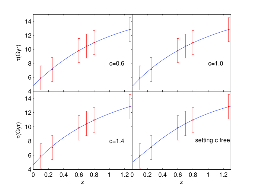
Figure 4: $\tau$ as a function of $z$ using the best fitting results. The data points with $1\sigma$ error bar are observational values.

We further find that the best fitting results for larger values of $c=1.0$ and $1.4$ are not consistent with the confidence regions derived from the differential ages of passively evolving galaxies, while that of case $c=0.6$ is within the $2\sigma$ confidence region. For the case setting $c$ free, the best fitting result from the lookback time method is in good agreement with the that from differential ages within 68.3% confidence region. Similar to the results from differential ages, the best fitting value of $h$ is also larger than the result of WMAP [29]. In addition, the values of $\chi_{\rm min}^{2}$ also reveals that there exist better fitting results for smaller $c$. Therefore, it seems that a smaller $c$ is more suitable.

We also calculate the corresponding errors $H$ and $t_{\rm L}$ derived from the differential ages of passively evolving galaxies. The error at different redshift $z$ can be expressed as

$$\sigma^{2}(z)=\sum^{K}_{i,j=1}\bigg{(}\frac{\partial y(z)}{\partial X_{i}}\frac{\partial y(z)}{\partial X_{j}}\bigg{)}_{X=\overline{X}}COV(\overline{X_{i}},\overline{X_{j}}),$$ (16)

where $K$ is the number of the fitting parameters, $y(z)$ the theoretical function (such as $H(z)$ and $t_{\rm L}(z)$ here), $X$ and $\overline{X}$ the vectors of fitting parameters and the best fitting values respectively and $COV$ is the covariance matrix. We plot in Fig.5 the $1\sigma$ and $2\sigma$ error bars for $H$ (the left panel) and $t_{\rm L}$ (the right panel) for the differential ages together with the best fitting results of $H$ and $t_{\rm L}$ from the lookback time to galaxy clusters and the age of the Universe. Clearly, the Hubble parameters derived from the two independent methods are quite consistent with each other. The corresponding values of $H$ derived from the lookback time to galaxy clusters and the age of the Universe is nearly within $1\sigma$ region during most of the considered redshift range. For $t_{\rm L}$, a good agreement between the results from two methods appear at both lower redshifts at $1\sigma$ level and at higher redshifts at $2\sigma$ level.

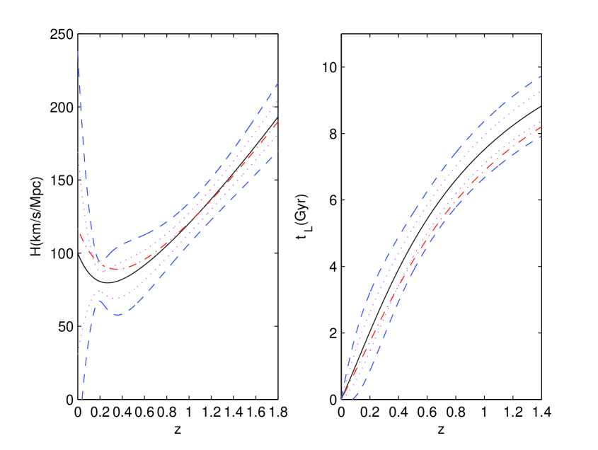
Figure 5: $H$(the left panel) and $t_{\rm L}$ (the right panel) as a function of redshift $z$. The solid curves stand for $H$ for best fitting values from the differential ages of passively evolving galaxies and the dash-dot curves represent $t_{\rm L}$ for best fitting values from the lookback time to galaxy clusters and the age of the Universe. The dashed and the dotted curves respectively correspond to $1\sigma$ and $2\sigma$ errors of $H$ and $t_{\rm L}$ from the differential ages.

5 The Deceleration Parameter and The Equation of State

The deceleration parameter is given in terms of $\Omega_{\rm H}$ like this [15,32],

$$q=\frac{1}{2}-\frac{1}{2}\Omega_{\rm H}-\frac{1}{c}\Omega_{\rm H}^{3/2},$$ (17)

which satisfies $-1/c\leq q\leq 1/2$ due to $0\leq\Omega_{\rm H}\leq 1$. We plot $q$ as a function of $z$ in Fig.6 using the best fitting values from the differential ages of passively evolving galaxies. Obviously $q$ start at the same point $q=1/2$ in the distant past for all cases of $c$, and the deceleration parameter is quite sensitive to $c$. Fig.6 also shows that the values of deceleration parameter today are $q_{\rm 0}$=-2.83, -0.98, -0.55 and -0.39 for $c$=0.26, 0.6, 1.0 and 1.4 respectively, which reveal that all the cases support a current accelerating Universe. And there exists a transition from deceleration to acceleration at $z_{\rm T}$=0.58, 0.71, 0.78 and 0.84 corresponding to $c$=0.26, 0.6, 1.0 and 1.4 respectively. The transition redshift $z_{\rm T}$ increases with the increase of $c$. More recent analysis also favor a lower transition [11,33-36]. In the work of Huang et al. [13], $z_{\rm T}$=0.28 and 0.72 for $c$=0.21 and 1.0 respectively. Therefore it seems that a smaller $c$ is more possible once again.

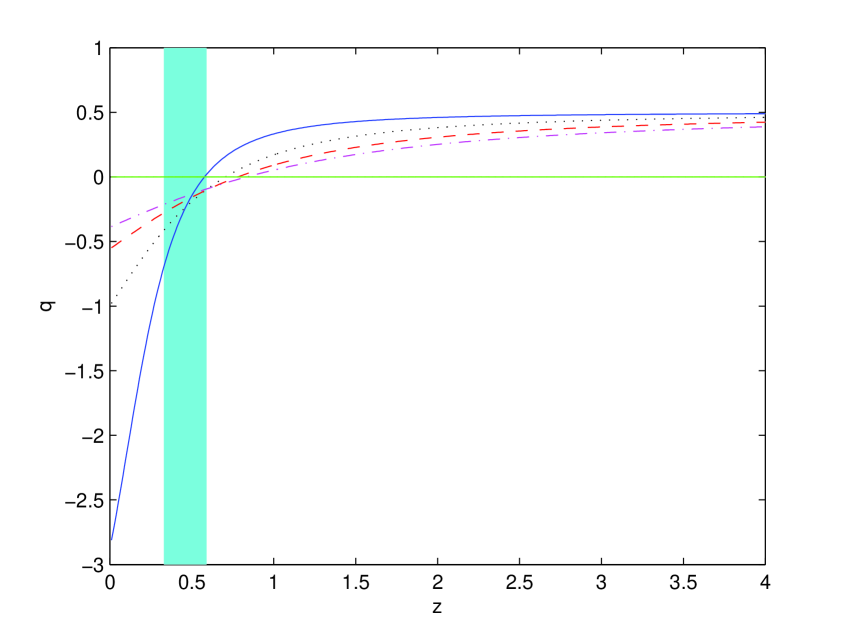
Figure 6: Deceleration parameter $q$ as a function of $z$. The dot line corresponds to $c=0.6$, $\Omega_{\rm m0}=0.24$, the dash $c=1.0$, $\Omega_{\rm m0}=0.23$ and the dash-dot $c=1.4$, $\Omega_{\rm m0}=0.21$ respectively. The solid line represents the case of setting $c$ free, $c=0.26$, $\Omega_{\rm m0}=0.16$ and the vertical shaded area indicates the SN Ia data constraint on the transition redshift ($z_{\rm T}=0.46\pm 0.13$) [28].

The equation of state is expressed in terms of $\Omega_{\rm H}$ like this [15,32],

$$\omega=-\frac{1}{3}(1+\frac{2}{c}\sqrt{\Omega_{\rm H}}).$$ (18)

It’s clear that $\omega$ evolves dynamically and $-(1+2/c)/3\leq\omega\leq-1/3$ due to $0\leq\Omega_{\rm H}\leq 1$. If $c>1.0$, it will always be larger than -1 so that the Universe avoids entering the de Sitter phase and the Big Rip phase [37]. If $c=1.0$, the holographic scenario will behave like the cosmological constant in the far future. However, if $c<1.0$, it will probably behave like a quintom-type dark energy whose equation of state is larger than -1 in the past while it’s less than -1 near today.

We plot $\omega$ as a function of $z$ in Fig.7 using the best fitting values from the differential ages of passively evolving galaxies. We find that at present $\omega_{\rm 0}$=-2.69, -1.30, -0.92 and -0.75 for $c$=0.26, 0.6, 1.0 and 1.4 respectively. In the work of Huang et al. [13], $\omega_{\rm 0}$=-2.67 and -0.91 for $c$=0.21 and 1.0, which is slightly larger than our result of $c$=0.26 and 1.0 respectively. Riess et al. [28] pointed out $\omega_{\rm 0}<-0.76$ at the 95.4% confidence level by using SN Ia data. This result is roughly consistent with our result of a smaller $c$.

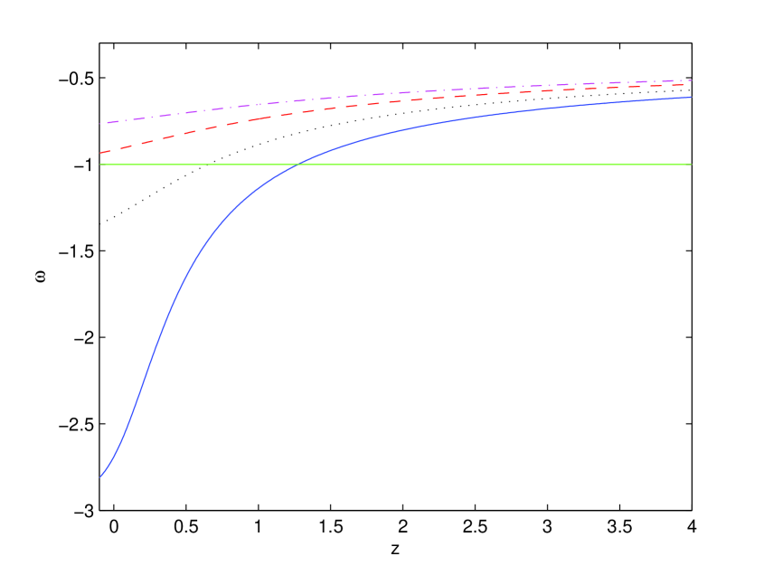
Figure 7: Same as Fig.6, but for the equation of state $\omega$.

6 Conclusions and Discussions

In this paper, we use the the measured Hubble parameters to present a constraint on a spatially flat Friedmann-Robert-Walker Universe with a matter component and a holographic dark energy component. Firstly we consider three fixed values of $c$=0.6, 1.0 and 1.4 in the fitting of data. If we set $c$ free, the best fitting values are $c=0.26$, $\Omega_{\rm m0}=0.16$, $h=0.9998$. It is shown that the holographic dark energy behaves like a quintom at the $1\sigma$ level although it is possible for $c>1.0$ at $95.4\%$ confidence level. This result is consistent with some other independent cosmological tests, which imply that $c<1.0$ is favored. We also test our results using the data of lookback time to galaxy clusters and the present age of the Universe. It is shown that the two independent methods are in better agreement if the fixed $c$ is smaller and the results from the two approaches for the case of setting $c$ free are roughly consistent. We claim that our method is acceptable and our results are reliable.

Their current values are $q_{\rm 0}=-2.83,-0.98,-0.55,-0.39$ and $\omega_{\rm 0}=-2.69,-1.30,-0.92,-0.75$ for $c$=0.26, 0.6, 1.0 and 1.4 respectively. The transition from deceleration to acceleration happened at $z_{\rm T}$=0.58, 0.71, 0.78, and 0.84 for $c$=0.26, 0.6, 1.0, and 1.4. Compared with the SN Ia observation [28], we find that a smaller $c$ is more acceptable.

It is important to note that this method is much more reliable than that based on absolute galaxy ages which is more sensitive to systematics errors [38,39]. Absolute galaxy ages can provide only a lower limit to the age of the Universe [38]. We are still faced with the problems of how to select the passively evolving galaxies, how to confirm the absolute ages and how to determine $\Delta z$. They are both sticking points but model-dependent, with unavoidable uncertainties. The data we use were obtained assuming a single-burst stellar population model and a single metallicity model. In fact, there may exist a serious warp. While the single metallicity approximation affects the recovered ages well below the error bars, the single-burst approximation may not work well generally. The star formation activity at low redshift for massive elliptical galaxies could bias the single-burst equivalent ages of the spectrum towards younger ages.

There still exist some deficiencies waiting for improving for our work. The amount of data for the differential ages of passively evolving galaxies is limited. The best fitting values $\Omega_{\rm m0}=0.16$ and $h=0.9998$ are far from the most known priors and the confidence regions in the $\Omega_{\rm m0}-c$ plane are not small enough. Probably the fitting result can be improved by combining other observational data.

References

- (1) [1] A. G. Riess et al. ApJ. 116, 1009 (1998)
- (2)
- (3) [2] J. L. Tonry et al. ApJ. 594, 1 (2003)
- (4)
- (5) [3] S. M. Carroll et al. hep-th/9207037
- (6)
- (7) [4] R. R. Caldwell et al. Phys. Rev. Lett. 80, 1582 (1998)
- (8)
- (9) [5] A. Y. Kamenshchik et al. Phys. Lett. B. 487, 7 (2000)
- (10)
- (11) [6] C. Csaki et al. Phys. Rev. D. 62, 045015 (2000)
- (12)
- (13) [7] K. Freese & M. Lewis. Phys. Lett. B. 540, 1 (2002)
- (14)
- (15) [8] A. G. Cohen et al. Phys. Rev. Lett. 82, 4971 (1999)
- (16)
- (17) [9] J. D. Bekenstein. Phys. Rev. D. 49, 1912 (1994)
- (18)
- (19) [10] L. Susskind. J. Math. Phys. 36, 6377 (1995)
- (20)
- (21) [11] Y. G. Gong. Class. Quant. Grav. 22, 2121 (2005)
- (22)
- (23) [12] M. Li. Phys. Lett. B. 603, 1 (2004)
- (24)
- (25) [13] Q. G. Huang & Y. G. Gong. JCAP. 0408, 006 (2004)
- (26)
- (27) [14] Z. Chang et al. Phys. Lett. B. 633, 14 (2006)
- (28)
- (29) [15] X. Zhang & F. Q. Wu. Phys. Rev. D. 72, 043524 (2005)
- (30)
- (31) [16] H. C. Kao et al. Model. Phys. Rev. D. 71, 123518 (2005)
- (32)
- (33) [17] J. Simon et al. Phys. Rev. D. 71, 123001 (2005)
- (34)
- (35) [18] R. Jimenez & A. Loeb. ApJ. 573, 37 (2002)
- (36)
- (37) [19] S. Capozziello et al. Phys. Rev. D. 70, 123501 (2004)
- (38)
- (39) [20] H. V. Peiris et al. ApJ. 148, 175 (2003)
- (40)
- (41) [21] R. G. Abraham et al. ApJ. 127, 2455 (2004)
- (42)
- (43) [22] T. Treu et al. MNRAS. 326, 221 (2001)
- (44)
- (45) [23] T. Treu et al. ApJL. 564, L13 (2002)
- (46)
- (47) [24] J. Dunlop et al. Nature. 381, 581 (1996)
- (48)
- (49) [25] H. Spinrad et al. ApJ. 484, 581 (1997)
- (50)
- (51) [26] P. L. Nolan et al. ApJ. 597, 615 (2003)
- (52)
- (53) [27] R. Jimenez et al. MNRAS. 349, 240 (2004)
- (54)
- (55) [28] A. G. Riess et al. ApJ. 607, 665 (2004)
- (56)
- (57) [29] D. N. Spergel et al. ApJS. 148, 175 (2003)
- (58)
- (59) [30] R. Rebolo et al. astro-ph/0402466, 2004
- (60)
- (61) [31] N. Dalal et al. Phys. Rev. Lett. 87, 141302 (2001)
- (62)
- (63) [32] B. Feng et al. Phys. Lett. B. 607, 35 (2005)
- (64)
- (65) [33] R. A. Daly & S. G. Djorgovski. ApJ. 612, 652 (2004)
- (66)
- (67) [34] U. Alam et al. MNRAS. 354, 275 (2004)
- (68)
- (69) [35] U. Alam et al. JCAP. 0406, 008 (2004)
- (70)
- (71) [36] H. K. Jassal et al. MNRAS. 356, L11 (2005)
- (72)
- (73) [37] D. Huterer & A. Cooray. Phys. Rev. D. 71, 023506 (2005)
- (74)
- (75) [38] J. S. Alcaniz & J. A. S. Lima. ApJ. 550, L133 (2001)
- (76)
- (77) [39] J. Dunlop et al. Nature. 381, 581 (1996)
- (78)