Systematic effects in the sound horizon scale measurements

Abstract

We investigate three potential sources of bias in distance estimations made assuming that a very simple estimator of the baryon acoustic oscillation (BAO) scale provides a standard ruler. These are the effects of the non-linear evolution of structure, scale-dependent bias and errors in the survey window function estimation. The simple estimator used is the peak of the smoothed correlation function, which provides a variance in the BAO scale that is close to optimal, if appropriate low-pass filtering is applied to the density field. While maximum-likelihood estimators can eliminate biases if the form of the systematic error is fully modeled, we estimate the potential effects of un- or mis-modelled systematic errors. Non-linear structure growth using the Smith et al. (2003) prescription biases the acoustic scale by $<0.3\%$ at $z\geq 1$ under the correlation-function estimator. The biases due to representative but simplistic models of scale-dependent galaxy bias are below $1\%$ at $z\geq 1$ for bias behaviour in the realms suggested by halo model calculations, which is expected to be below statistical errors for a $1000$ sq. degs. spectroscopic survey. The distance bias due to a survey window function errors is given in a simple closed form and it is shown it has to be kept below $2\%$ not to bias acoustic scale more than $1\%$ at $z=1$, although the actual tolerance can be larger depending upon galaxy bias. These biases are comparable to statistical errors for ambitious surveys if no correction is made for them. We show that RMS photometric zero-point errors (at limiting magnitude $25$ mag) below $0.14$ mag and $0.01$ mag for redshift $z=1$ (red galaxies) and $z=3$ (Lyman-break galaxies), respectively, are required in order to keep the distance estimator bias below $1\%$.

1 Introduction

Acoustic oscillations in the plasma during the pre-recombination epoch have been detected in the cosmic microwave background (CMB) (Spergel et al., 2003). Moreover, these oscillations should be imprinted on the distribution of matter in the Universe and survive until the present epoch. The presence of these oscillations was detected as a ‘hump’ in the correlation function of Luminous Red Galaxies (LRG) sample in the Sloan Digital Sky Survey (SDSS) (Eisenstein et al., 2005), with some evidence in the power spectrum of galaxy distribution in the 2dF Galaxy Redshift Survey (Cole et al., 2005). These pioneering measurements reveal the potential of future galaxy surveys, larger and deeper than present ones, to measure the sound horizon scale as a function of redshift for epochs up to the present day. The physics of the plasma era are well understood and let us compute the sound horizon in absolute units (e.g. meters). BAO measurements may become the best modern incarnation of standard cosmological tests based on a standard ruler, for determining the expansion history of the Universe and/or in tests for curvature (Bernstein, 2006).

Not much is known, however, about possible systematic effects which could make the measurement of the sound horizon more difficult than expected. The purpose of this paper is to quantify the bias in the sound horizon scale introduced by effects like nonlinear evolution, scale-dependent bias in tracer objects distribution and observational selection (window function). We compare these levels of potential systematic error to statistical uncertainties expected for future hemisphere-scale galaxy surveys. Is the baryon peak in the correlation function a robust measure of a distance once set in place by physics in the pre-recombination era?

Figure 1: The nonlinear dark matter power spectrum (upper panel) and respective correlation function (lower panel) for our fiducial cosmological model at the redshift $z=1$. Baryon acoustic oscillations are seen as wiggles in the power spectrum and the ‘hump’ at scale $102.1\;\,h^{-1}\mathrm{Mpc}$ in the correlation function. For scales larger than the baryon acoustic peak the correlation function becomes negative (dashed line).

Quantitative examination of biases in BAO distance estimation require that we specify the means by which a single distance estimation will be extracted from the surveyed galaxy distribution in some redshift range. The existing literature on the precision of BAO estimates considers the distance-estimation problem in Fourier space (Seo & Eisenstein, 2003; Blake & Glazebrook, 2003; Angulo et al., 2005; Blake et al., 2006; Seo & Eisenstein, 2005), where the BAO signature is a set of “baryon wiggles” appearing in the galaxy power spectrum at scales $0.01\,h\,\mathrm{Mpc}^{-1}\la k\la 0.5\,h\,\mathrm{Mpc}^{-1}$. A model power spectrum, uncertain by a scale factor, is fit to the observed galaxy power spectrum. In the limit where the galaxy distribution is Gaussian and the model power spectrum is exactly specified by theory, this yields the maximum-likelihood estimator for the characteristic scale and hence an unbiased, minimum-variance estimation. If effects such as nonlinear growth or galaxy bias are correctly incorporated into the model, then the maximum-likelihood techniques still yield optimal unbiased estimators. It may remain infeasible, however, to model all effects exactly or even know their functional forms, so we must consider the potential systematic biases from mis-modelled physical effects, or those that are not modelled at all. Most current BAO analyses or forecasts incorporate additional free parameters, typically in the form of “smooth” functions of $k$ that add to or multiply the baseline “wiggly” model, in an attempt to mimic any kind of broadband systematic effect (Seo & Eisenstein, 2003; Tegmark et al., 2006). Marginalization over the nuisance smooth-function parameters yields the single acoustic-scale estimator.

The Fourier-domain marginalization technique somewhat obscures the means by which the estimator may end up being biased. The situation is much clearer in real space, where the linear-era BAO signature is a 3-dimensional Green’s function comprising a central peak with a spherical shell of radius $r_{s}$, the acoustic horizon scale (Eisenstein et al., 2006). This clearly produces a single peak at $r_{s}$ in the real-space correlation function. We therefore choose to make the location of this correlation-function peak our estimator and use this very simple estimator to gauge the magnitude of biases from unmodelled systematic errors. We will demonstrate that this simple estimator is not far from optimal, and hence it is useful to quantify its biases. This simple estimator incorporates no particular model for non-linearity or galaxy biasing; hence by calculating the degree of bias these effects generate in this estimator, we have a worst-case estimate. Future analysis of the detailed physics will be capable of generating corrections that reduce these biases.

We choose the correlation-function peak to be as model independent as possible and avoid the obscuration of fitting a smooth function to the power spectrum. The appearance of the baryon peak in the correlation function at scales $\simeq 100\;\,h^{-1}\mathrm{Mpc}$ is difficult to mimic with the small-scale effects which can obscure the higher-order wiggles in the power spectrum. The power spectrum analysis is appealing due to the independence of evolution of Fourier modes (at least in the linear regime), but the correlation-function peak also has a simple statistical analysis in the Gaussian limit.

As this work was completed, Eisenstein et al. (2006) published an excellent overview of the relation between the Fourier- and real-space views of acoustic oscillations in both the linear and non-linear regimes. While their work focusses on developing an analytical and physical understanding of the BAO non-linearities and biasing, we will take the opposite and less challenging approach of using toy models and halo models for non-linear effects, which may not be physically accurate, but yield bias estimates that are sufficiently quantitative to identify biases that are most in need of further attention.

The fiducial cosmology is the same as in Blake et al. (2006) to facilitate comparison: flat $\Lambda$CDM with total matter density $\Omega_{m}=0.3$ and baryon fraction $f_{b}=15\%$. The present Hubble parameter is taken to be $h=0.7$ in units of $100\;\mathrm{km/s/Mpc}$, power spectrum normalization $\sigma_{8}=1$ and the primordial spectral index $n_{s}=1$. We use the linear transfer function given by Eisenstein & Hu (1998). Nonlinear corrections to the power spectrum are based on the fitting formula given by Smith et al. (2003) or the halo model (Cooray & Sheth, 2002). The nonlinear fitting formula was inferred from results of the pure dark matter simulations (the halo model is also usually calibrated with N-body simulations) and it is not a priori clear that it is very precise for the case of nonzero baryon contribution. The matter power spectrum and respective correlation function for our fiducial model are shown in Fig. 1 where a ‘hump’ around the scale $100\,h^{-1}\mathrm{Mpc}$ is the BAO feature. Changing cosmological parameters makes the ‘hump’ scale, amplitude and width change accordingly (Matsubara, 2004). A fast and reliable transformation between the Fourier and the real space can be performed by means of the FFTLog routines (Hamilton, 2000).

Our analysis is simplified in the sense that we work in real space without distinguishing between transverse and radial directions and we do not take redshift space distortions into account. The former assumption means that both tangential and radial directions are taken to scale the same with the angular-diameter distance $D_{A}(z)$, so information about $D_{A}(z)$ might be obtained from either direction. In other words we assume that accurate spectroscopic redshifts are available for sources with negligible peculiar velocities, and that the product of the angular-diameter distance and the Hubble parameter $D_{A}(z)H(z)$ is known rather than having $D_{A}(z)$ and $H(z)$ measured independently. These assumptions are unrealistic, but should not spoil the rough estimates of bias from physical effects other than redshift-space distortion.

2 Statistical errors on the sound horizon scale

Before addressing the bias in the correlation-function estimator of $r_{s}$, we analyse the estimator’s statistical errors due to the finite survey volume $V_{s}$ (sample variance) and finite density of observed objects $n_{g}$ (shot noise).

Errors associated with sample variance scale roughly with the comoving survey volume as $V_{s}^{-1/2}$ (Tegmark, 1997). In the “concordance” $\Lambda$CDM model (Spergel et al., 2003), the comoving volume of space available for observations which cover the whole sky grows from $2.4\,h^{-3}\mathrm{Gpc}^{3}$ for $z\leq 0.3$, through $52\,h^{-3}\mathrm{Gpc}^{3}$ for $z\leq 1$ up to $284\,h^{-3}\mathrm{Gpc}^{3}$ for $z\leq 2.5$. For this reason, as well as the degradation of the BAO feature by nonlinearities at $z<1$, the statistical power of BAO surveys degrades significantly at $z<1$, although see Eisenstein et al. (2006) for a potential strategy to ameliorate the second effect.

All of the statistical errors on BAO estimators scale with $V_{s}^{-1/2}$. For illustrative purposes we will consider volumes contained in very wide redshift bins, $\Delta z=0.5$. Proposals exist for near-term surveys to cover $\sim 1000$ sq. degs. of the sky, for which a redshift bin $\Delta z=0.5$ centred at $z=1$ gives an observable volume $V_{s}=1.4\,h^{-3}\mathrm{Gpc}^{3}$, twice as much as used by SDSS collaboration to discover the baryon acoustic peak. A highly ambitious goal would be a spectroscopic BAO survey covering half of the sky, for a survey volume of $28\,h^{-3}\mathrm{Gpc}^{3}$ in the $z=1$ bin. We will term these the “modest-scale” and “hemisphere-scale” survey scenarios.

The shot noise comes from the finite number of objects sampling the distribution of mass. With finite resources (telescope time) a survey of the baryon peak has to be balanced between volume and sampling density to obtain maximal signal to noise ratio. As elaborated by Seo & Eisenstein (2003) and Matsubara (2004) these considerations typically lead to a relation between the optimal number density of objects $n_{g}$ and their power spectrum $P(k)$ in the form $n_{g}P(k)\sim 1$. In the case of BAO we will assume $n_{g}P(k=0.2\,h\,\mathrm{Mpc}^{-1})=3$ (Seo & Eisenstein, 2003), unless specified otherwise. For $z=1$ we obtain $n_{g}=2.5\times 10^{-3}\,h^{3}\mathrm{Mpc}^{-3}$ if galaxies are unbiased relative to the mass distribution. In sec. 4.1 we will consider galaxy bias and its effect on the baryon acoustic peak.

In order to compute statistical errors in the sound horizon scale measurement let us consider the behaviour of the galaxy correlation function $\xi_{g}$ about its peak at $r\simeq 100\,h^{-1}\mathrm{Mpc}$. The characteristic scale where the peak in the correlation function is observed will be denoted $r_{c}$ and is an estimator, possibly biased, of the sound horizon scale $r_{s}$. We allow for smoothing of the observed galaxy distribution with a window $W_{R}(k)$ with a characteristic scale $R$ to suppress the small scale power (i.e. mostly the shot noise) which contributes to the noise but not to the BAO signal in the correlation function. Next, let us compute the derivative $F(r)$ of the correlation function as an integral over the power spectrum:

$$F(r)={d\xi_{g}\over dr}=-\frac{1}{2\pi^{2}}\int\;dkk^{3}P(k)W^{2}_{R}(k)j_{1}(kr),$$ (1)

where $j_{m}(x)$ is a spherical Bessel function of the $m$-th order. The position of the characteristic peak is given by $F(r_{c})=0$. Thus uncertainty in its position is given by

$$\sigma_{r_{c}}=\frac{\sigma_{F}}{|\partial F/\partial r|},$$ (2)

taken at $r=r_{c}$. From eq. (1) we obtain the variance of $F(r_{c})$ as

$$\sigma^{2}_{F}=\frac{2}{2\pi^{2}V_{s}}\int\;dkk^{4}\sigma^{2}_{P}(k)W^{4}_{R}(k)j^{2}_{1}(kr_{c}),$$ (3)

where $\sigma^{2}_{P}(k)$ is the variance of a single mode of the power spectrum, given by $\sigma^{2}_{P}(k)=\left(P(k)+1/n_{g}\right)^{2}$ (Feldman et al., 1994; Tegmark, 1997). Hence, the statistical uncertainty on the position of the characteristic scale $r_{c}$ is given by

$$\sigma^{2}_{r_{c}}=\frac{\sigma^{2}_{F}}{\left[\int dk\;k^{4}P(k)W^{2}_{R}(k)\left(j_{0}(kr_{c})-\frac{2}{kr_{c}}j_{1}(kr_{c})\right)\right]^{2}},$$ (4)

where $\sigma^{2}_{F}$ is given by eq. (3). We adopt a Gaussian filter of the form $W_{R}(k)=e^{-k^{2}R^{2}/2}$, i.e. we presume the galaxy density field to be smoothed with a Gaussian of width $R$ before measuring the correlation function.

Figure 2: Relative statistical error of the characteristic scale $r_{c}$ in the real space correlation function vs. filtering scale $R$. Note the competing effects of the shot noise subtraction (small $R$) and baryon wiggles removal (large $R$), both due to the smoothing. Shown are predictions for the modest 1000 sq. degs. survey covering volume of $1.4\,h^{-3}\mathrm{Gpc}^{3}$ around $z=1$ ($\Delta z=0.5$) and spatial galaxy density (solid lines, from top to bottom) $2.5\times 10^{-3}\,h^{3}\mathrm{Mpc}^{-3}$, $12.5\times 10^{-3}\,h^{3}\mathrm{Mpc}^{-3}$, $25\times 10^{-3}\,h^{3}\mathrm{Mpc}^{-3}$. The dashed line is the sample-variance-limited case. For the full-hemisphere survey, all values should scaled with survey volume as $V_{s}^{-1/2}$, lowering errors by a factor of 4.5. Nonlinear evolution has been modelled with the Smith et al. (2003) prescription.

In Fig. 2 we show statistical errors $\sigma(r_{c})/r_{c}$ in the baryon-peak position, computed by means of eq. (4), vs the smoothing scale $R$, for the modest-scale survey at redshift $z=1$. The statistical errors on the hemisphere survey are expected to be $4.5$ times smaller.

The choice of smoothing scale is a trade between beating down the shot noise and affecting the BAO signal when smoothing is too aggressive—smoothing with $R=7\,h^{-1}\mathrm{Mpc}$ makes the peak disappear into a “knee” in the correlation function. A smoothing scale of $R=3\,h^{-1}\mathrm{Mpc}$ seems to yield a signal to noise close to optimal for different shot noise contributions (see Fig. 2), so we adopt this value for the remainder of our analysis.

The smoothing procedure shifts the position of the peak in the correlation function, biasing the recovered characteristic scale $r_{c}$. For our assumed $R=3\;\,h^{-1}\mathrm{Mpc}$ filter the bias is $-0.8\%$. This will not be a concern in the course of this work because we are only interested in relative changes of the peak position with redshift. Furthermore, we could in practice correct the peak shift using theoretical spectra and knowledge of the smoothing procedure.

The expected errors for the acoustic scale are similar to those claimed by Blake et al. (2006). In Table 1 we present a concise comparison between expected errors of our the peak-of-the-correlation function approach (PCF) and of the power spectrum approach of Blake et al. (2006) (B2006). Because Blake et al. (2006) consider errors in tangential and radial acoustic scale separately, we add them in inverse quadrature and these combined errors are shown in Table 1. The errors are shown for the modest-scale and the hemisphere-scale surveys around the redshift $z=1$ with a depth $\Delta z=0.5$. Also, two cases of sampling density are considered, one where $n_{g}=2.5\times 10^{-3}\,h^{3}\mathrm{Mpc}^{-3}$ which is implied by the “optimality” condition $n_{g}P(k=0.2\,h\,\mathrm{Mpc}^{-1})=3$, the other with zero shot noise contribution. We notice that the former case equals to almost sample variance limited. The statistical errors implied by the PCF method are the same as obtained by B2006 in the case of the modest-scale survey and only $3\%$ smaller for the hemisphere-scale one, assuming $n_{g}=2.5\times 10^{-3}\,h^{3}\mathrm{Mpc}^{-3}$. One may infer from this comparison that the PCF method of the sound horizon estimation works well although the estimate of errors is likely too optimistic (see Sec. 1).

Table 1: Fractional errors on the estimated acoustic scale for different surveys obtained be means of the peak-of-the-correlation function method (PCF) described in this paper and the power spectrum results of Blake et al. (2006) (B2006). The surveys are assumed to be around the redshift $z=1$ and to have the depth $\Delta z=0.5$. We applied a usual smoothing scale $R=3\,h^{-1}\mathrm{Mpc}$.

	$1000\;\mathrm{sq.~{}degs.}$		$1/2$ sky
	$V_{s}=1.4\,h^{-3}\mathrm{Gpc}^{3}$		$V_{s}=29\,h^{-3}\mathrm{Gpc}^{3}$
$n_{g}[\,h^{3}\mathrm{Mpc}^{-3}]$	PCF	B2006	PCF	B2006
$2.5\times 10^{-3}$	$1.5\%$	$1.5\%$	$0.32\%$	$0.31\%$
$\infty$	$1.2\%$	$1.1\%$	$0.27\%$	$0.24\%$

Because the peak-of-correlation-function estimator is nearly as precise as maximum-likelihood power-spectrum-fitting techniques, it is worthwhile to use this simple model-independent estimator to investigate bias properties.

3 Effects of nonlinear evolution

The nonlinear evolution of matter perturbations in the Universe and its effect on the baryon wiggles in the power spectrum have been studied using numerical simulations (e.g. Meiksin et al. (1999); Springel et al. (2005); Seo & Eisenstein (2005)). Nonlinear evolution couples Fourier modes of the matter distribution, suppresses power at intermediate scales ($k\sim 0.05\,h\,\mathrm{Mpc}^{-1}$), amplifies power at small scales $k\ga 0.1\,h\,\mathrm{Mpc}^{-1}$ and partially erases the baryon wiggles. This degrades the precision of BAO measurements for given survey volume, although Eisenstein et al. (2006) suggest that some of this degradation is reversible using corrections for bulk flows.

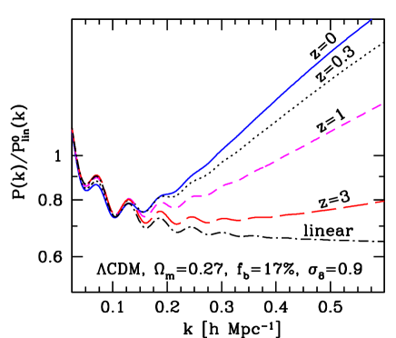
Figure 3: The ratio of the nonlinear matter power spectrum for a model with baryon fraction $f_{b}=17\%$, total matter density $\Omega_{m}=0.27$ and $\sigma_{8}=0.9$ to the CMB normalised linear power spectrum $P^{0}_{\mathrm{lin}}(k)$ with no baryons for redshifts $z=3$ (long dashed), $z=1$ (short dashed), $z=0.3$ (dotted), $z=0$ (solid). The normalised linear power spectrum is also shown (dot dashed). Nonlinear evolution modelling in based on the Smith et al. (2003) fitting formula and can be compared to the numerical results of Seo & Eisenstein (2005) in their Fig. 1. Note that the cosmological model assumed here differs from the one used throughout the paper.

Numerical simulations have not, however, been useful for estimating biases in BAO estimators, because they remain too noisy in the range of scales interesting from the point of view of baryon wiggles, roughly from $k\sim 0.01\;\,h\,\mathrm{Mpc}^{-1}$ through $k\sim 0.5\;\,h\,\mathrm{Mpc}^{-1}$ (Springel et al., 2005). To estimate the bias in a survey of given volume, the simulation volume must be significantly larger than the survey volume. Sufficient resources have not yet been available to simulate volumes comparable to those to be surveyed by a hemisphere-scale survey at $z>1$, for example.

One must hence at present rely on analytic arguments to investigate the bias of BAO distance estimations. We base our analysis of nonlinear effects on a fitting formula proposed by Smith et al. (2003) which was inspired by the halo model and calibrated with N-body numerical simulations. We include the effects associated with baryons in the formula via the linear transfer function (Eisenstein & Hu, 1998). The validity of this description of nonlinear evolution has not yet been tested extensively, although the formula is able to describe reasonably the characteristic features in the power spectra of simulations that include baryons. In Fig. 3 we show predictions for the power spectrum behaviour given by the fitting formula, which can be compared to the numerical results of Seo & Eisenstein (2005). Our plot can be compared to their Fig. 1; the overall shape of the power spectrum is recovered reasonably well, however the wiggles, especially those from the third one on, seem to be more prominent (less erased) in our description than in the simulations.

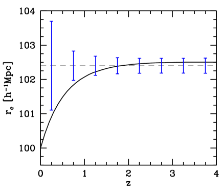
Figure 4: Effect of the nonlinear matter evolution on the measured sound horizon scale from the real space correlation function. We plot the characteristic scale position $r_{c}$ as a function of redshift for our fiducial cosmological model (solid line). The horizontal line (dashed) shows the characteristic scale for the linear matter evolution, $r_{c}=102.4\,h^{-1}\mathrm{Mpc}$. The error bars represent statistical errors in the baryon-peak position from the hemisphere-scale survey, assuming that we use galaxies lying in bins of width $\Delta z=0.5$.

The influence of nonlinear effects on the measured characteristic scale $r_{c}$ is shown in Fig. 4. The bias versus the linear-regime value of $r_{c}=102.4\,h^{-1}\mathrm{Mpc}$ is negative for small redshifts and positive for large ones and for sufficiently early epochs becomes zero. For epochs earlier than $z=1.5$, the bias in the sound horizon scale is $<0.1\%$ and below the statistical error for the hemisphere-scale survey. At redshift $z=1$ the fractional bias is $\Delta r_{c}/r_{c}=-0.3\%$, very close to the expected statistical errors from the hemisphere-scale survey at that epoch. For redshifts smaller than $z=1$ the nonlinear evolution begins to affect first two baryon wiggles, and the bias approaches $\Delta r_{c}/r_{c}=-2.4\%$ at $z=0$. In the $0<z<1$ range, the bias is comparable to the statistical errors in the hemisphere-scale survey. Hence the non-linearity bias would not greatly dominate the error budget for any feasible survey at any redshift range, and in fact would be unimportant for any survey that does not approach hemisphere scale. This is true even without having made any correction to the estimator to account for nonlinearities.

It is worth mentioning that the bias due to the influence of dark energy on the growth of structure (McDonald et al., 2005) is negligible.

4 The galaxy bias and the baryon-peak position

The distribution of galaxies is a biased tracer of mass distribution and depends on the type of galaxies considered (Zehavi et al., 2005; Marinoni et al., 2005). In order to quantify the effect of galaxy bias on the measured sound horizon scale, we must specify the scale dependence of the bias which, unfortunately, is poorly known at present. One commonly describes the galaxy bias in terms of the multiplicative factor $b(k)$ relating matter power spectrum $P_{m}(k)$ and the galaxy one $P_{g}(k)$ as $P_{g}(k)=b^{2}(k)P_{m}(k)$. Obviously any bias that is independent of scale leaves the location of the peak in the correlation function unchanged.

4.1 The galaxy bias in the halo model

The halo model is a statistical description of the structure of the Universe based on two basic observations: on large scales the matter evolution can be described by perturbative models and on small scales matter clusters into bound haloes of a given profile (see Cooray & Sheth (2002) for a review). The matter and galaxy 2-point functions are divided into two-halo and one-halo terms, so the matter and galaxy power spectra become

$$P_{m,g}(k) = P_{\mathrm{lin}}(k)\left(\int dMb_{h}(M)n_{h}(M)w^{(2)}_{m,g}u_{m,g}(k)\right)^{2}$$ (5)

$$+\int dMn_{h}(M)w^{(1)}_{m,g}u^{2}_{m,g}(k),$$

where $b_{h}$ is the halo bias, $n_{h}$ is the halo mass function, $u_{m}(k)$ ($u_{g}(k)$) is the normalised mass (galaxy) distribution profile of a halo of mass $M$ in the Fourier space. The weight functions for matter and galaxy power spectra have the following form for the two-halo term $w^{(2)}_{m}=M/\bar{\rho}$, $w^{(2)}_{g}=\left<N\right>/\bar{n}_{g}$ and for the one-halo term $w^{(1)}_{m}=M^{2}/\bar{\rho}^{2}$, $w^{(1)}_{g}=\left<N(N-1)\right>/\bar{n}_{g}^{2}$, respectively. $N$ is the number of galaxies of a given type occupying a halo of mass $M$. A form of first and second moments of distribution of $N$ must be specified and depends on the means of populating haloes with galaxies.

The relation between the mean number of galaxies $\left<N\right>$ in a given halo and the halo mass $M$ is dubbed the halo occupation distribution (HOD). Usually, the HOD for luminosity-threshold samples is described by: the minimum mass $M_{\mathrm{min}}$ of a halo in which galaxies may form; the mass $M_{1}$ of a halo which contain one satellite galaxy on average; and the slope $\alpha$ of the relation between number of satellite galaxies per halo of a given mass: $\left<N(M)\right>=\left(1+\left(M/M_{1}\right)^{\alpha}\right)H(M-M_{\mathrm{min}})$, where $H$ is a step function. The details of the halo model parameterisation we use can be found in Hu & Jain (2004). In this framework we can obtain the galaxy bias as a function of scale and galaxy type provided that we know the HOD. The specific form of an HOD was first suggested by theoretical studies (Seljak, 2000; Berlind & Weinberg, 2002; Kravtsov et al., 2004; Zheng et al., 2005).

Given the galaxy bias, $b(k)=\sqrt{P_{g}(k)/P_{m}(k)}$, or equivalently the galaxy spectrum $P_{g}(k)$, from the halo model, we can calculate the correlation function and hence the characteristic scale $r_{c}$ of its peak. In this halo-model calculation, one finds that non-linear growth and biasing does not bias the baryon-peak position $r_{c}$ at all (within numerical errors which are about $0.1\%$ in $r_{c}$) for halo mass thresholds up to $\sim 100M_{\star}$. This makes sense when one realizes that in the halo model the acoustic oscillations are present only in the two-halo term, which is assumed to be proportional to the linear matter power spectrum, eq. (5). The one-halo term is completely featureless at the acoustic scale unless one considers extremely massive haloes, so the peak of the correlation function is unchanged. Another way to state this is that the halo-model $b^{2}(k)$ has small oscillations, coherent with the baryon oscillations, that arrange to leave the correlation peak unchanged. The scale dependent galaxy bias from the halo model was considered by Schulz & White (2006). Thorough analysis of the halo bias, based on the perturbation theory and numerical simulations, was presented recently in Smith et al. (2006). Their approach extends the standard halo model by accounting for higher order corrections to the linear power spectrum and relaxing a common assumption of the linear, scale independent bias in the two-halo term. They also discuss potential impact of these improvements on the BAOs.

The near-exact invariance of the correlation function peak may be considered a peculiarity of the halo model. More sophisticated halo models (Sheth et al., 2001; Yang et al., 2003; Zheng, 2004; Tinker et al., 2005) account for the effect of previrialisation in the power spectrum which the standard model of eq. (5) fails to describe properly. It is usually done by replacing the linear matter power spectrum with the nonlinear one in eq. (5) and accounting for halo exclusion in the two-halo term. We do not introduce these improvements in our present analysis because the resultant shifts in the PCF are those we ascribed to non-linear growth in Sec. 3, e.g. Fig. 4. In this section we wish to isolate PCF shifts due solely to scale-dependent bias, so we opt to describe the nonlinear bias by a generic smooth function, (see Sec. 4.2) that does not share the halo model’s exceptional behaviour, and is simply described by the maximum and minimum bias values and the $k$ range over which the bias varies. We will use the halo model to determine reasonable ranges for these generic parameters, and then estimate the shift of the correlation-function peak for the reasonable generic functions.

A three-parameter family of HODs allows one to model accurately the projected correlation function of low-redshift galaxies ($z\la 0.07$) from the Sloan Digital Sky Survey (Zehavi et al., 2005). These authors obtain a good fit to the projected correlation function when $M_{1}/M_{\mathrm{min}}\simeq 23$, almost independent of the luminosity threshold of galaxies in a sample. At the same time $\alpha$ rises from $0.9$ to $1.2$ with luminosity. The modelling of the SDSS galaxy correlation function is done assuming that the distribution of galaxies within dark matter haloes follow the distribution of the matter.

Unfortunately, such a detailed modelling of an HOD is not available for more distant galaxies so we have to base our considerations for redshift $z\ga 0.1$ on results obtained from numerical simulations. Hydrodynamical simulations carried by Zheng et al. (2005) broadly support the picture which emerges from already mentioned the SDSS galaxy clustering data (Zehavi et al., 2005). The former show that both characteristic masses, $M_{\mathrm{min}}$ and $M_{1}$, scale similarly with galaxy baryonic mass and their ratio for $z=0$ is $M_{1}/M_{\mathrm{min}}\simeq 14$. Although the numeric value of the ratio differs from the one obtained from the SDSS galaxy sample, the scaling of $M_{\mathrm{min}}$ and $M_{1}$ with galaxy baryonic mass (simulations) and luminosity (observations) is very similar. On the other hand, dark-matter-only simulations conducted by Kravtsov et al. (2004) show that the relation between number of subhaloes and the mass of the host halo is almost linear ($\alpha=1$) in a very wide range of halo masses ($M_{1}/M_{\mathrm{min}}\ga 3$) and for cosmic epochs $z\la 5$. Another important result of these simulations is quantifying an evolution of the ratio $M_{1}/M_{\mathrm{min}}$ with redshift that implies $M_{1}/M_{\mathrm{min}}\simeq 29$ for $z=0$, $M_{1}/M_{\mathrm{min}}\simeq 19$ for $z=1$ and $M_{1}/M_{\mathrm{min}}\simeq 17$ for $z=3$ (see Fig. 5 in Kravtsov et al. (2004)).

Encouraged by the success of the halo model in describing the galaxy clustering we use it for the description of the galaxy bias. In this work we consider two HOD models, one parameterised by $M_{\mathrm{min}}$, $M_{1}$ and $\alpha$ as mentioned above (“central+satellite” scheme) and the other where number of galaxies in a given halo is proportional to its mass for haloes more massive than $M_{\mathrm{min}}$ (similar to the “mass weighted” scheme of Seo & Eisenstein (2005)). The main differences between those two schemes are the following. In the “central+satellite” description if there is at least one galaxy in a halo then exactly one galaxy is at the halo centre whereas in “mass weighted” scheme all galaxies are distributed within a halo. This implies that in the former case the small scale power is boosted by the presence of the galaxy in the centre, in the latter case small scale power is “smoothed” in a way similar to the dark matter distribution. These effects are shown in Fig. 5 where we present the galaxy bias at $z=1$ as a function of scale assuming those two schemes of populating haloes with galaxies. The threshold mass $M_{\mathrm{min}}$ is chosen to be $0.1M_{\star}$, $M_{\star}$ or $10M_{\star}$ where $M_{\star}=8\times 10^{11}h^{-1}M_{\odot}$. We note that the bias in the case of “mass weighted” scheme shows a rapid change on scales which are potentially relevant for a behaviour of the baryon wiggles ($k$ around a few tenths of $\,h\,\mathrm{Mpc}^{-1}$). This is because the most rapid change in the bias appears where the galaxy power spectrum is becoming dominated by the one-halo term, whereas the matter power spectrum is steep (slope $\sim-1.5$) in this regime. These circumstances appear at different scales, depending on the parameterisation of the HOD and the galaxy distribution, as seen in Fig. 5.

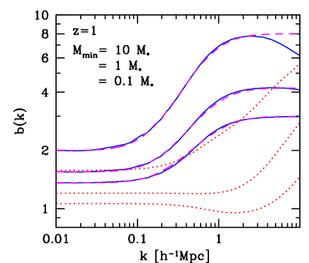
Figure 5: The galaxy bias from the halo model for two schemes of populating haloes with galaxies: when number of galaxies occupying a halo is proportional to the halo mass (solid lines), and when there are central and satellites galaxies with $M_{1}=20M_{\mathrm{min}}$ (dotted lines). The minimum mass of the haloes inhabited by galaxies for each occupation scheme are $0.1M_{\star}$, $M_{\star}$ and $10M_{\star}$ (from bottom to top for each family of curves). Redshift $z=1$ is assumed for which $M_{\star}=8\times 10^{11}h^{-1}M_{\odot}$. The bias relation as given by the generic function described in Sec. 4.2 is overplotted (dashed lines).

4.2 A toy model

The halo model confines us to the very specific outcome of zero systematic which the Universe may not exhibit. We should therefore investigate what possible form of the galaxy bias would imply substantial change in the baryon-peak position. As mentioned in Sec. 4.1 the scale dependence of the galaxy bias in the “mass weighted” case as shown in Fig. 5 can be described in the interesting range of scales ($0.01\,h\,\mathrm{Mpc}^{-1}\la k\la 1\,h\,\mathrm{Mpc}^{-1}$) as a smoothed step-like function. A good description can be provided by the function of the following form

$$\log b^{2}(k)=\left|\log\frac{b_{+}}{b_{-}}\right|\;\mathrm{erf}\left[\frac{\log k/k_{m}}{\sqrt{2}\Delta_{\sigma}}\right]+\log\left(b_{+}b_{-}\right),$$ (6)

where we use the error function and characterise the bias $b(k)$ by its asymptotic values at large and small scales, $b_{-}$ and $b_{+}$, respectively (when $b_{+}/b_{-}>1$ we have bias, in the other case – antibias). In our analysis it is the ratio $b_{+}/b_{-}$ which is important as multiplying the power spectrum by a constant factor does not change the position of the peak but its amplitude only. The other parameters are the scale $k_{m}$ where the most rapid change of the bias occurs, and the logarithmic interval in $k$, $\Delta_{\sigma}$, centred on $k_{m}$, over which the bias changes by $68.3\%$. A simple function should suffice if we are trying to recover trends in the baryon-peak bias due to the galaxy bias and not to obtain its precise values. We exclude situations where the bias has a functional form containing oscillations of any kind (which was the case in the halo model description, see Fig. 5). We expect that the most prominent effect on the baryon-peak position occurs when the bias changes rapidly on scales where baryon wiggles are present in the power spectrum, $0.01\;\,h\,\mathrm{Mpc}^{-1}\la k\la 0.5\;\,h\,\mathrm{Mpc}^{-1}$.

We now check whether the baryon-peak of the correlation function is a robust measure of the sound horizon in the presence of scale-dependent, smooth deviations in the power spectrum. In Fig. 6 we present results of applying the galaxy bias of a form given by eq. (6) to the linear matter power spectrum. The typical scale of the bias change is fixed to $\Delta_{\sigma}=0.4$, as suggested by the halo model. We take into account only the “mass weighted” case as the “central+satellite” scheme introduces negligible bias to the acoustic scale.

The largest effect can be introduced by the galaxy bias when the most rapid change in bias takes place around the first baryon wiggle in the power spectrum ($k_{m}\simeq 0.02\,h\,\mathrm{Mpc}^{-1}$) which itself overlaps the matter power spectrum turnover. The correlation-function peak shift persists to $k\simeq 0.08\,h\,\mathrm{Mpc}^{-1}$, around the second peak. It is difficult to imagine that the bias has a very rapid change on scales as large as the matter power spectrum turnover, which is roughly equal to the largest scale of possible physical interactions in the pre-recombination Universe. For scales $k_{m}\simeq 0.5\,h\,\mathrm{Mpc}^{-1}$, where it is more reasonable to consider scale dependence of the galaxy bias, a very strong bias amplitude of order several is required to change the baryon-peak position by more than $2\%$. If we look to the halo model for an estimate of the amplitude of scale-dependent bias, we find the shift in the characteristic scale $r_{c}$ is below 1% at $z=1$ for any threshold mass below $3M_{\star}$ (the survey depth is $\Delta z=0.5$). The halo-model parameters for our toy model further suggest that, for surveys of galaxies inhabitating haloes of mass $M_{\star}$ a bias of the acoustic peak is $0.7\%$ at the redshift $z=1$, whereas expected statistical error for the modest-scale survey is $1.5\%$. For redshifts $z=2$ and $z=3$ respective systematic errors are $0.5\%$ and $0.2\%$ and statistical ones $1\%$ and $0.95\%$. Statistical errors for the hemisphere-scale survey are smaller by a factor of $4.5$. The bias becomes comparable to statistical errors for the hemisphere-scale survey, but not for the modest-scale one. This is without any correction to the estimator $r_{c}$. Numerical models should eventually allow for corrections to reduce the bias below statistical errors ever for hemisphere-scale surveys.

It is difficult to assign the minimum halo mass that will correspond to future BAO galaxy surveys at $z\ga 1$. It will depend on the selection criteria for galaxies in the future surveys. Haloes of mass $\ga M_{\star}$ are possible hosts of SDSS Luminous Red Galaxies at $z\sim 0.3$ (Zehavi et al., 2005). Similar studies of halo occupancy have yet to be done at higher $z$, but the appropriate halo-model mass threshold $M_{\mathrm{min}}$ will likely be in the range $0.1-10M_{\star}$.

When estimating statistical errors we assumed no galaxy bias. In practice, the bias is likely to help in lowering statistical errors either through allowing for a denser sampling or covering larger area while using the same resources.

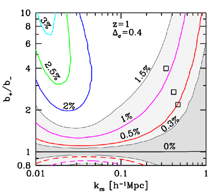
Figure 6: Contour plot of the fractional bias of the baryon-peak position as a function of scale $k_{m}$ at which the most rapid change of the galaxy bias appears and the relative amplitude of the galaxy bias $b_{+}/b_{-}$. The range of scales where bias changes the most rapidly is fixed to $\Delta_{\sigma}=0.4$. Open squares mark values of parameters which describe by means of the smooth function the galaxy bias obtained from the halo model (see Fig. 5) assuming minimal halo masses of $0.1M_{\star}$, $M_{\star}$, $10M_{\star}$ (from bottom to top). Shaded regions show parts of the parameter space where statistical errors on baryon-peak position dominate over the systematic shift. Statistical errors are assumed to be for two surveys: the modest-scale (light shaded region) and the hemisphere-scale (dark shaded region).

5 Survey window function

Another effect which requires attention is the possible influence of the survey selection function on the baryon-peak position in the correlation function. Let us assume that the observers of our fictitious real-space survey have estimated a spatial selection function $W_{0}(\vec{r})$, but the correct selection function differs by a small multiplicative correction $\delta_{W}(\vec{r})$. The observed galaxy density will be

$$\rho_{g}(\vec{r})=n_{g}W_{0}(\vec{r})\left(1+\delta_{W}(\vec{r})\right)\left(1+\delta_{\mathrm{true}}(\vec{r})\right).$$ (7)

The experimenters will estimate the overdensity using their estimated selection function, so will calculate an (incorrect) local overdensity

$$\left(1+\delta_{\mathrm{obs}}(\vec{r})\right)=\left(1+\delta_{W}(\vec{r})\right)\left(1+\delta_{\mathrm{true}}(\vec{r})\right).$$ (8)

The observers’ calculated correlation function $\xi_{\rm obs}$ follows:

$$1+\xi_{\mathrm{obs}}(r)=\left(1+\xi_{W}(r)\right)\left(1+\xi_{\mathrm{true}}(r)\right),$$ (9)

where we assume that the selection function is uncorrelated with the true density field, and $\xi_{W}$ is the autocorrelation of the fractional errors $\delta_{W}$ in the selection-function estimate.

What level of residuals in the window function are allowed in order not to bias the sound horizon scale determination more than predicted statistical errors? We are interested in scales which are close to the baryon peak in the correlation function, so we can approximate correlation function $\xi_{\mathrm{true}}(r)$ to second order about the true acoustic scale

$$\xi_{\mathrm{true}}(r)=\xi_{\mathrm{true}}(r_{s})\left(1-\frac{\left(r-r_{s}\right)^{2}}{2\sigma^{2}_{0}}\right).$$ (10)

$\sigma^{2}_{0}$ has an interpretation as the width of the baryon peak. The characteristic scale $r_{c}$ is measured from the position of the peak in the observed function $\xi_{\mathrm{obs}}(r)$, so the derivative of the $\xi_{\mathrm{obs}}$ is zero at $r_{c}$. Hence the shift in the baryon-peak position due to the presence of spatially-varying error in the selection function is

$$\delta r_{s}\equiv r_{c}-r_{s}=-\left[\ln\left(1+\xi_{W}(r_{c})\right)\right]^{\prime}\frac{\left(1+\xi_{\mathrm{true}}(r_{s})\right)}{\xi^{\prime\prime}_{\mathrm{true}}(r_{s})},$$ (11)

where the prime means the derivative with respect to $r$ and only linear terms in $\delta r_{s}$ are retained in the expression for $\xi_{\mathrm{true}}$. Note the bias depends only upon the properties of $\xi_{W}$ at the acoustic scale.

From eqs. (10) and (11) follows that for the power law $\xi_{W}(r)$ with an exponent $-\alpha$ and an amplitude $\xi_{W}\ll 1$ in the vicinity of the observed peak we obtain to the leading order

$$\frac{\delta r_{s}}{r_{s}}=-\alpha\left(\frac{\sigma_{0}}{r_{s}}\right)^{2}\frac{\xi_{W}(r_{c})}{\xi_{\mathrm{true}}(r_{s})}.$$ (12)

The narrower the acoustic peak, the less easily it is moved; and the shallower $\xi_{W}(r)$ is at the acoustic scale, the smaller a bias in the peak position is produced.

We can make an estimate of the level of systematic errors due to the unknown properties of the window function for a given survey. As an example let us consider the survey at the redshift $z\simeq 1$ in which case we had $r_{s}=102.1\,h^{-1}\mathrm{Mpc}$, $\xi_{\mathrm{true}}(r_{s})=6.33\times 10^{-4}$ and $\sigma_{0}=10.2\,h^{-1}\mathrm{Mpc}$ where we assume no galaxy bias (Sec. 2) and $\alpha=2$. Thus eq. (12) implies that to be able to beat down the systematic error to the level of $\delta r_{s}/r_{s}$, e.g. $1\%$, the correlation function of the window function correction cannot be larger than

$$\left|\xi_{W}(r_{c})\right| = 3.2\times 10^{-4}\left(\frac{\xi_{\mathrm{true}}(r_{s})}{6.33\times 10^{-4}}\right)\left(\frac{\sigma_{0}}{10.2\,h^{-1}\mathrm{Mpc}}\right)^{-2}$$ (13)

$$\times\left(\frac{\alpha}{2}\right)^{-1}\left(\frac{r_{s}}{102.1\,h^{-1}\mathrm{Mpc}}\right)^{2}\left|\frac{\delta r_{s}/r_{s}}{1\%}\right|.$$

Hence, eq. (13) shows that unknown variation in the selection function on scales of the baryon peak should be $\la 1.8\%$ if we want to bias our results no more than $1\%$. For larger redshifts the allowed variation would have to be smaller — $1.3\%$ and $1\%$ for $z=2$ and $3$, respectively. Scaling of the variation with redshift is mainly due to the linear suppression of the mass fluctuations and narrowing of the baryon peak (several times smaller effect). A survey of biased galaxies makes $\xi_{\mathrm{true}}(r_{s})$ rise, allowing for a larger error in the selection function without biasing $r_{c}$ by more than the statistical error.

An example of an effect which can bring about correlations on large scales considered above is the extinction pattern on the sky which is known to be correlated on scales of tens of degrees (Schlegel et al., 1998). Also, for surveys around redshift $z=1(3)$ the acoustic scale is about $2.5(1.3)$ deg (as opposed to $\sim 6$ deg for the SDSS LRG sample). This is around (or less) than a size of a field of view of planned wide-field surveys, thus a different magnitude limit for each telescope pointing may introduce correlations on the interesting scale (Guzik & Bernstein, 2005). Moreover, significant uncertainty to a measured window function may be introduced by a complicated geometry of a survey (Miller et al., 2002; Cole et al., 2005).

We investigate a model in which each telescope pointing has an independent magnitude calibration error, and relate the RMS magnitude error to the systematic bias on the baryon peak position through the survey window function as assumed in eq. (8). The correlation function of the angular window function for calibration errors in circular fields of diameter $\theta_{a}$ is (Guzik & Bernstein, 2005) $\xi_{W}(\theta)=2/\pi\Sigma^{2}(\arccos(\theta/\theta_{a})-(\theta/\theta_{a})\sqrt{1-(\theta/\theta_{a})^{2}})$ if $\theta\leq\theta_{a}$ and zero otherwise. Now let us compute the variance, $\Sigma^{2}$, which is given as a fractional uncertainty in the density of objects in the real space due to the survey limiting magnitude error

$$\sqrt{\Sigma^{2}}=\frac{\delta(n_{g}W_{0})}{n_{g}W_{0}}=\frac{\phi(L/L_{\star})\frac{dL}{dm}}{\int_{L/L_{\star}}^{\infty}\phi(L/L_{\star})dL/L_{\star}}|_{m_{\mathrm{lim}}}\delta m,$$ (14)

where $\phi(L)$ is the luminosity function in the Schechter form $\phi(L)dL=\phi_{\star}(L/L_{\star})^{\alpha}\exp(-L/L_{\star})d(L/L_{\star})$ and $m_{\mathrm{lim}}$ is a survey limiting magnitude. For a survey of red (blue) galaxies at $z\simeq 1.1$ (Faber et al., 2005) the luminosity function is described by a characteristic density of $\phi_{\star}=1.5(8.4)\times 10^{-3}(\,h^{-1}\mathrm{Mpc})^{-3}$, characteristic absolute magnitude $M_{\star}=-21.58(-21.25)$ and the faint-end slope $\alpha=-0.5(-1.3)$. At $z\simeq 3$, observations of Lyman-break galaxies (Steidel et al., 1999) yield $\phi_{\star}=48.0\times 10^{-3}(\,h^{-1}\mathrm{Mpc})^{-3}$, $M_{\star}=-21.68$, $\alpha=-1.6$. Also, let us assume that the survey telescope aperture is $\theta_{a}=3$ deg and the limiting apparent magnitude is $25$ mag. A predicted position of the baryon peak at $z=1(3)$ (see Sec. 1) is $102.1(102.5)\,h^{-1}\mathrm{Mpc}$, its width $10.2(9.5)\,h^{-1}\mathrm{Mpc}$ and the matter correlation function amplitude at the peak scale $6.33(3.16)\times 10^{-4}$. Then from eq.(11) we obtain that the magnitude calibration error $\delta m$ should be smaller than $0.14(0.05)\times b^{2}$ for survey of red (blue) galaxies at $z\simeq 1$ if we require an error on the baryon peak position be smaller than $1\%$. Note that the calibration depends on the galaxy bias $b$. Respective calibration error for $z\simeq 3$ yields $0.01\times b^{2}$. If we extrapolate results of Padmanabhan et al. (2006) to the bias of Luminous Red Galaxies to $z\simeq 1$ we could expect the bias of this type of galaxies is $b\simeq 2$. Blue galaxies are expected to be much less biased (Zehavi et al., 2005). Thus, the magnitude calibration for the redshift survey of the red galaxy sample at $z\simeq 1$ should not present any practical challenge. The considered effect can have more impact on the blue-galaxy sample due to the steeper faint end of their luminosity function. Also, for a survey at $z\simeq 3$, the required calibration accuracy may be more difficult to obtain, although a large bias, of order a few or more (Porciani & Giavalisco, 2002; Kashikawa et al., 2006), can help. Predictions for $z\simeq 3$ can vary because the limiting magnitude is on the exponential part of the luminosity function.

6 Conclusions

We have considered three types of possible systematic effects in the estimation of the cosmological distances by means of the baryon acoustic peak in the correlation function. Our analysis accounts for the nonlinear evolution of structure, the galaxy biasing with respect to the underlying mass and the effect of imperfect recovery of the survey selection function. In each of these cases we compare systematic to statistical errors that one could expect for a $1000$ sq. degs. and a half of the sky spectroscopic surveys.

The nonlinear evolution biases the estimated acoustic scale for redshift $z\la 1.5$. For redshift $z=1$ (and the depth of the survey $\Delta z=0.5$) the systematic error is $0.3\%$ and grows up to $2.4\%$ at $z=0$, close to the predicted statistical errors for the hemisphere-scale survey. Statistical errors are expected to dominate the systematic ones for any survey smaller than this, e.g. the modest-scale survey yields statistical errors larger by a factor of $4.5$ than the hemisphere-scale one. Thus, the effect of the nonlinear evolution on the measured acoustic scale is expected to be below statistical errors for $z\ga 1$ in case of planned surveys even without applying correction for nonlinear evolution. Correction techniques, like the one proposed by Eisenstein et al. (2006), may be useful in unbiasing the acoustic scale even for shallow surveys, $z\ll 1$.

The measured acoustic scale may also be affected by the scale-dependent galaxy bias which is poorly known at present. We quantified a possible effect of the galaxy bias based on the toy model supported by the halo model results. We showed that for the case of the galaxy bias predicted by the halo model it is unlikely to introduce systematic effect on acoustic scale exceeding $1\%$ when haloes of mass $\la 3M_{\star}$ at the redshift $z=1$ are considered. For less massive haloes the acoustic scale bias is smaller. In fact, the bias for $M_{\star}$ haloes at $z=1$ is $0.7\%$ which is lower by a factor of $2$ than statistical errors for the modest-scale survey ($1.5\%$) and higher than those expected for the hemisphere-scale survey ($0.3\%$). For higher redshifts, the acoustic scale bias for $M_{\star}$ haloes is expected to be at least a factor of $2.5(4.75)$ smaller than the statistical errors for the redshift $z=2(3)$ in case of the modest-scale survey. On the other hand, the systematic error could be larger if the change of the bias with scale was more rapid or took place at larger scales than suggested by the halo model.

Also, we considered the bias in the acoustic scale measurement due to the correlated errors in the survey window function. In our analysis the systematic error depends linearly upon the local slope of the correlation function of the selection function residuals and varying inversely with the local curvature of the true correlation function. Our analysis implies that in order to achieve a bias $<1\%$ one has to measure the window function (more precisely, $\xi_{W}(\sim 100\,h^{-1}\mathrm{Mpc})$) with accuracy better than $2\%$ at $z=1$, and more accurately for higher redshifts. The constraint can be relaxed if the galaxy bias on scales of the acoustic peak is greater than 1. Specific results depend on details of a survey and a data reduction methods. We considered one model, namely independent photometric zero-point errors at each telescope pointing. RMS zero-point errors (at limiting magnitude $25$ mag) below $0.14$ mag and $0.01$ mag for redshift $z=1$ (red galaxies) and $z=3$ (Lyman-break galaxies), respectively, are required in order to limit systematic error in the peak-of-the-correlation-function estimator to less than $1\%$. In order to gain a confidence in unbiasedness of the acoustic scale measurement, techniques to diagnose window function problems have to be developed and applied (Tegmark et al., 2002).

We compared the variance of the peak-of-the-correlation function estimator to the power spectrum estimator (Blake et al., 2006) and found the former yields virtually the same statistical inaccuracies as the latter. This suggests that our model-independent estimator might be useful in measuring of the sound horizon scale in spite of the simplifying assumptions we made in the course of its analysis. Even though its variance may turn out to be larger, its simplicity and model independence are sufficient reasons for the peak-of-the-correlation method to be practically important.

In this paper we considered only the real space correlation function. In the redshift space, a peak in the correlation function becomes an elliptical ridge and one has to properly modify the peak-of-the-correlation function estimator to become applicable in this case. Fortunately, the large scale redshift space distortions (Kaiser, 1987) do not lead to a bias of the baryon-peak position because the relation between an azimuthally averaged redshift space power spectrum and the real space one is scale independent. However, an improved analysis of redshift space distortions (Seljak, 2001; Scoccimarro, 2004) may lead to different implications. We defer an analysis of the redshift space effects to the future work.

References

- Angulo et al. (2005) Angulo R., Baugh C. M., Frenk C. S., Bower R. G., Jenkins A., Morris S. L., 2005, MNRAS, 362, L25
- Berlind & Weinberg (2002) Berlind A. A., Weinberg D. H., 2002, ApJ, 575, 587
- Bernstein (2006) Bernstein G., 2006, ApJ, 637, 598
- Blake & Glazebrook (2003) Blake C., Glazebrook K., 2003, ApJ, 594, 665
- Blake et al. (2006) Blake C., Parkinson D., Bassett B., Glazebrook K., Kunz M., Nichol R. C., 2006, MNRAS, 365, 255
- Cole et al. (2005) Cole S. et al., 2005, MNRAS, 362, 505
- Cooray & Sheth (2002) Cooray A., Sheth R., 2002, Phys. Rep., 372, 1
- Eisenstein & Hu (1998) Eisenstein D. J., Hu W., 1998, ApJ, 496, 605
- Eisenstein et al. (2006) Eisenstein D. J., Seo H.-j., White M., 2006, astro-ph/0604361
- Eisenstein et al. (2005) Eisenstein D. J. et al., 2005, ApJ, 633, 560
- Faber et al. (2005) Faber S. M. et al., 2005, astro-ph/0506044
- Feldman et al. (1994) Feldman H. A., Kaiser N., Peacock J. A., 1994, ApJ, 426, 23
- Guzik & Bernstein (2005) Guzik J., Bernstein G., 2005, Phys. Rev. D, 72, 043503
- Hamilton (2000) Hamilton A. J. S., 2000, MNRAS, 312, 257
- Hu & Jain (2004) Hu W., Jain B., 2004, Phys. Rev. D, 70, 043009
- Kaiser (1987) Kaiser N., 1987, MNRAS, 227, 1
- Kashikawa et al. (2006) Kashikawa N. et al., 2006, ApJ, 637, 631
- Kravtsov et al. (2004) Kravtsov A. V., Berlind A. A., Wechsler R. H., Klypin A. A., Gottlöber S., Allgood B., Primack J. R., 2004, ApJ, 609, 35
- Marinoni et al. (2005) Marinoni C. et al., 2005, A&A, 442, 801
- Matsubara (2004) Matsubara T., 2004, ApJ, 615, 573
- McDonald et al. (2005) McDonald P., Trac H., Contaldi C., 2005, astro-ph/0505565
- Meiksin et al. (1999) Meiksin A., White M., Peacock J. A., 1999, MNRAS, 304, 851
- Miller et al. (2002) Miller C. J., Nichol R. C., Chen X., 2002, ApJ, 579, 483
- Padmanabhan et al. (2006) Padmanabhan N. et al., 2006, astro-ph/0605302
- Porciani & Giavalisco (2002) Porciani C., Giavalisco M., 2002, ApJ, 565, 24
- Schlegel et al. (1998) Schlegel D. J., Finkbeiner D. P., Davis M., 1998, ApJ, 500, 525
- Schulz & White (2006) Schulz A. E., White M., 2006, Astroparticle Physics, 25, 172
- Scoccimarro (2004) Scoccimarro R., 2004, Phys. Rev. D, 70, 083007
- Seljak (2000) Seljak U., 2000, MNRAS, 318, 203
- Seljak (2001) Seljak U., 2001, MNRAS, 325, 1359
- Seo & Eisenstein (2003) Seo H.-J., Eisenstein D. J., 2003, ApJ, 598, 720
- Seo & Eisenstein (2005) Seo H.-J., Eisenstein D. J., 2005, ApJ, 633, 575
- Sheth et al. (2001) Sheth R. K., Hui L., Diaferio A., Scoccimarro R., 2001, MNRAS, 325, 1288
- Smith et al. (2003) Smith R. E. et al., 2003, MNRAS, 341, 1311
- Smith et al. (2006) Smith R. E., Scoccimarro R., Sheth R. K., 2006, astro-ph/0609547
- Spergel et al. (2003) Spergel D. N. et al., 2003, ApJS, 148, 175
- Springel et al. (2005) Springel V. et al., 2005, Nat, 435, 629
- Steidel et al. (1999) Steidel C. C., Adelberger K. L., Giavalisco M., Dickinson M., Pettini M., 1999, ApJ, 519, 1
- Tegmark (1997) Tegmark M., 1997, Physical Review Letters, 79, 3806
- Tegmark et al. (2006) Tegmark M. et al., 2006, astro-ph/0608632
- Tegmark et al. (2002) Tegmark M., Hamilton A. J. S., Xu Y., 2002, MNRAS, 335, 887
- Tinker et al. (2005) Tinker J. L., Weinberg D. H., Zheng Z., Zehavi I., 2005, ApJ, 631, 41
- Yang et al. (2003) Yang X., Mo H. J., van den Bosch F. C., 2003, MNRAS, 339, 1057
- Zehavi et al. (2005) Zehavi I. et al., 2005, ApJ, 630, 1
- Zheng (2004) Zheng Z., 2004, ApJ, 610, 61
- Zheng et al. (2005 ) Zheng Z. et al., 2005, ApJ, 633, 791