Cosmology with clusters of galaxies

1 Introduction

Clusters of galaxies occupy a special place in the hierarchy of cosmic structures. They arise from the collapse of initial perturbations having a typical comoving scale of about 10$\,h^{-1}{\rm Mpc}$. According to the standard model of cosmic structure formation, the Universe is dominated by gravitational dynamics in the linear or weakly non–linear regime and on scales larger than this. In this case, the description of cosmic structure formation is relatively simple since gas dynamical effects are thought to play a minor role, while the dominating gravitational dynamics still preserves memory of initial conditions. On smaller scales, instead, the complex astrophysical processes, related to galaxy formation and evolution, become relevant. Gas cooling, star formation, feedback from supernovae (SN) and active galactic nuclei (AGN) significantly change the evolution of cosmic baryons and, therefore, the observational properties of the structures. Since clusters of galaxies mark the transition between these two regimes, they have been studied for decades both as cosmological tools and as astrophysical laboratories.

In this Chapter I concentrate on the role that clusters play in cosmology. I will highlight that, in order for them to be calibrated as cosmological tools, one needs to understand in detail the astrophysical processes which determine their observational characteristics, i.e. the properties of the cluster galaxy population and those of the diffuse intra–cluster medium (ICM).

Constraints of cosmological parameters using galaxy clusters have been placed so far by applying a variety of methods. For example:

1. The mass function of nearby galaxy clusters provides constraints on the amplitude of the power spectrum at the cluster scale (e.g., 2002ARA&A..40..539R ; 2005RvMP…77..207V and references therein). At the same time, its evolution provides constraints on the linear growth rate of density perturbations, which translate into dynamical constraints on the matter and Dark Energy (DE) density parameters.

2. The clustering properties (i.e., correlation function and power spectrum) of the large–scale distribution of galaxy clusters provide direct information on the shape and amplitude of the underlying DM distribution power spectrum. Furthermore, the evolution of these clustering properties is again sensitive to the value of the density parameters through the linear growth rate of perturbations (e.g., 2001Natur.409…39B ; 2001MNRAS.327..422M and references therein).

3. The mass-to-light ratio in the optical band can be used to estimate the matter density parameter, $\Omega_{m}$, once the mean luminosity density of the Universe is known and under the assumption that mass traces light with the same efficiency both inside and outside clusters (see 2000ApJ…541….1B ; 2000ApJ…530…62G ; 1996ApJ…462…32C , as examples of the application of this method).

4. The baryon fraction in nearby clusters provides constraints on the matter density parameter, once the cosmic baryon density parameter is known, under the assumption that clusters are fair containers of baryons (e.g., 1991MNRAS.253P..29F ; 1993Natur.366..429W ). Furthermore, the baryon fraction of distant clusters provide a geometrical constraint on the DE content and equation of state, under the additional assumption that the baryon fraction within clusters does not evolve (e.g., 2002MNRAS.334L..11A ; 2003A&A…398..879E ).

An extensive presentation of all these methods would probably require a dedicated book. For this reason, in this contribution I will mostly concentrate on the method based on the evolution of the cluster mass function. A substantial part of my Lecture will concentrate on the different methods that have been applied so far to weight galaxy clusters. Since all the above cosmological applications rely on precise measurements of cluster masses, this part of my contribution will be of general relevance for cluster cosmology.

Also, since most of the cosmological applications of galaxy clusters have been based so far on X–ray surveys, my discussion will be definitely X–ray biased, although I will discuss in some detail methods based on optical observations and what present and future optical surveys are expected to provide. I refer to the Lectures by R. Gal and O. Lopez–Cruz in this volume for more details regarding the properties of galaxy clusters in the optical band. Also, I will refer to the Lectures by M. Birkinshaw for cosmological studies of clusters based on the Sunyaev–Zeldovich (SZ) effect, to the Lectures by J.–P. Kneib for cluster studies and mass measurement through gravitational lensing, and to the Lectures by C. Jones and by C. Sarazin for more details about the cosmological application of the baryon fraction method.

The structure of this Chapter will be as follows. I provide in Section 2 a short introduction to the basics of cosmic structure formation. I will shortly review the linear theory for the evolution of density perturbations and the spherical collapse model. In Section 3 I will describe the Press–Schechter (PS) formalism to derive the cosmological mass function. I will then introduce extensions of the PS approach and present the most recent calibrations of the mass function from N–body simulations. In Section 4 I will review the methods to build samples of galaxy clusters, based on optical and X–ray observations, while I will only briefly discuss the SZ methodology for cluster surveys. Section 5 is devoted to the discussion of different methods to derive cluster masses and to review the results of the application of these methods. In Section 6 I will describe the cosmological constraints, which have been obtained so far by tracing the cluster mass function with a variety of methods: distribution of velocity dispersions, X–ray temperature and luminosity functions, and gas mass function. In this Section I will also critically discuss the reasons for the different, sometimes discrepant, results that have been obtained in the literature and I will highlight the relevance of properly including the analysis of the cluster mass function all the statistical and systematic uncertainties in the relation between mass and observables. Finally, I will describe in Section 7 the future perspectives for cosmology with galaxy clusters and which are the challenges for clusters to keep playing an important role in the era of precision cosmology.

2 A concise handbook of cosmic structure formation

In this section I will briefly review the basic concepts of cosmic structure formation, which are relevant for the study of galaxy clusters as tools for precision cosmology through the evolution of their mass function. A complete treatment of models of structure formation can be found in classical cosmology textbooks (e.g., 1993ppc..book…..P ; 1999coph.book…..P ; 2002coec.book…..C ).

2.1 The statistics of cosmic density fields

Let $\rho(\rm{\bf x})$ be the matter density field, which is a continuous function of the position vector $\rm{\bf x}$, $\bar{\rho}={\left<\right.}\rho{\left.\right>}$ its average value computed over a sufficiently large (representative) volume of the Universe and

$$\delta(\rm{\bf x})={\rho(\rm{\bf x})-\bar{\rho}\over\bar{\rho}}$$ (1)

the corresponding relative density contrast. By definition, it is $\bar{\delta}=0$ and $\delta(\rm{\bf x})\geq-1$. If the density field is traced by a discrete distribution of points (i.e., galaxies or galaxy clusters) all having the same weight (mass), then $\rho(\rm{\bf x})=\sum_{i}\delta_{D}(\rm{\bf x}-\rm{\bf x}_{i})$, where $\delta_{D}(\rm{\bf x})$ is the Dirac delta–function. The Fourier representation of the density contrast is given by

$$\tilde{\delta}(\rm{\bf k})={1\over(2\pi)^{3/2}}\int d\rm{\bf x}\,\delta(\rm{\bf x})e^{i\rm{\bf k}\cdot\rm{\bf x}}\,,$$ (2)

with the corresponding dual relation for the inverse Fourier transform.

The 2–point correlation function for the density contrast is defined as

$$\xi(r)={\left<\right.}\delta(\rm{\bf x}_{1})\delta(\rm{\bf x}_{2}){\left.\right>}\,,$$ (3)

which only depends on the modulus of the separation vector, $r=|\rm{\bf x}_{1}-\rm{\bf x}_{2}|$, under the assumption of statistical isotropy of the density field. Therefore, it can be shown that the power spectrum of the density fluctuations is the Fourier transform of the correlation function, so that

$$P(k)={\left<\right.}|\tilde{\delta}(\rm{\bf k})|^{2}{\left.\right>}={1\over 2\pi^{2}}\int dr\,r^{2}\xi(r){\sin kr\over kr}\,,$$ (4)

which, again, depends only on the modulus of the wave-vector $\rm{\bf k}$.

In case we are interested in the study of a class of observable structures of mass $M$, which arise from the collapse of initial perturbations having size $R\propto(M/\bar{\rho})^{1/3}$, then it is common to introduce the smoothed density field, which is defined as

$$\delta_{R}(\rm{\bf x})=\delta_{M}(\rm{\bf x})=\int\delta(\rm{\bf y})W_{R}(|\rm{\bf x}-\rm{\bf y}|)\,d\rm{\bf y}\,.$$ (5)

As such, it is given by the convolution of the density fluctuation field with a window function, which filters out the fluctuation modes having wavelength $\raise-2.0pt\hbox{\hbox to0.0pt{\hbox{$\sim$}\hss}\raise 5.0pt\hbox{$<$}\ }R$. Eq.(5) allows us to introduce the variance of the fluctuation field computed at the scale R, defined as

$$\sigma^{2}_{R}=\sigma^{2}_{M}={\left<\right.}\delta_{R}^{2}{\left.\right>}={1\over 2\pi^{2}}\int dk\,k^{2}P(k)\,\tilde{W}_{R}^{2}(k)\,,$$ (6)

where $\tilde{W}_{R}(k)$ is the Fourier transform of the window function.

The shape of the window function defines the exact relation between mass and smoothing scale. For instance, for the top–hat window it is

$$\tilde{W}_{R}(k)={3[\sin(kR)-kR\cos(kR)]\over(kR)^{3}}$$ (7)

while the Gaussian window gives

$$\tilde{W}_{R}(k)=\exp\left(-{(kR)^{2}\over 2}\right),.$$ (8)

The corresponding relations between mass scale and smoothing scale are $M=(4\pi/3)R^{3}\bar{\rho}$ and $M=(2\pi R^{2})^{3/2}\bar{\rho}$ for the top–hat and Gaussian filters, respectively.

The shape of the power spectrum is (essentially) fixed once the matter density parameter, $\Omega_{m}$, that associated to the baryonic component, $\Omega_{\rm bar}$, and the Hubble parameter, $H_{0}$, are specified (e.g., 1999ApJ…511….5E ). However, its normalization can only be fixed through a comparison with observational data of the large–scale structure of the Universe or of the anisotropies of the Cosmic Microwave Background (CMB). A common way of parametrizing this normalization is through the quantity $\sigma_{8}$, which is defined as the variance, computed for a top–hat window having comoving radius $R=8\,h^{-1}{\rm Mpc}$ (given in eq. 6). The historical reason for this choice of the normalization scale is that the variance of the galaxy number counts, within the first redshift surveys, was observed to be about unity inside spheres of that radius (e.g., 1983ApJ…267..465D ). In this way, the value of $\sigma_{8}$ for a given cosmology directly provides a measure of the biasing parameter relating the galaxy and mass distribution, expected for that model. Furthermore, a top–hat sphere of $8\,h^{-1}{\rm Mpc}$ radius contains a mass $M\simeq 5.9\times 10^{14}\Omega_{m}\,h^{-1}M_{\odot}$, which is the typical mass of a moderately rich galaxy cluster. Therefore, as we shall see in Section 3, the mass function of galaxy clusters provides a direct measure of $\sigma_{8}$.

2.2 The linear evolution of density perturbations

Let us assume that the matter content of the Universe is dominated by a pressurless and self–gravitating fluid. This approximation holds if we are dealing with the evolution of the perturbations in the dark matter (DM) component or in case we are dealing with structures whose size is much larger than the typical Jeans scale–length of baryons. Let us also define $\rm{\bf x}$ to be the comoving coordinate and $\rm{\bf r}=a(t)\rm{\bf x}$ the proper coordinate, $a(t)$ being the cosmic expansion factor. Furthermore, if $\rm{\bf v}=\dot{\rm{\bf r}}$ is the physical velocity, then $\rm{\bf v}=\dot{a}\rm{\bf x}+\rm{\bf u}$, where the first term describes the Hubble flow, while the second term, $\rm{\bf u}=a(t)\dot{\rm{\bf x}}$, gives the peculiar velocity of a fluid element which moves in an expanding background.

In this case the equations that regulate the Newtonian description of the evolution of density perturbations are the continuity equation:

$${\partial\delta\over\partial t}+\nabla\cdot[(1+\delta)\rm{\bf u}]=0\,,$$ (9)

which gives the mass conservation, the Euler equation

$${\partial\rm{\bf u}\over\partial t}+2H(t)\rm{\bf u}+(\rm{\bf u}\cdot\nabla)\rm{\bf u}=-{\nabla\phi\over a^{2}}\,,$$ (10)

which gives the relation between the acceleration of the fluid element and the gravitational force, and the Poisson equation

$$\nabla^{2}\phi=4\pi G\bar{\rho}a^{2}\delta$$ (11)

which specifies the Newtonian nature of the gravitational force. In the above equations, $\nabla$ is the gradient computed with respect to the comoving coordinate $\rm{\bf x}$, $\phi(\rm{\bf x})$ describes the fluctuations of the gravitational potential and $H(t)=\dot{a}/a$ is the Hubble parameter at the time $t$. Its time–dependence is given by $H(t)=E(t)H_{0}$, where

$$E(z)=[(1+z)^{3}\Omega_{m}+(1+z)^{2}(1-\Omega_{m}-\Omega_{DE})+(1+z)^{3(1+w)}\Omega_{DE}]^{1/2}$$ (12)

is related to the density parameter contributed by non–relativistic matter, $\Omega_{m}$, and by Dark Energy (DE), $\Omega_{DE}$, with equation of state $p=w\rho c^{2}$ (if the DE term is provided by cosmological constant then $w=-1$).

In the case of small perturbations, these equations can be linearized by neglecting all the terms which are of second order in the fields $\delta$ and $\rm{\bf u}$. In this case, after further differentiating eq.(9) with respect to time, using the Euler equation to eliminate the term $\partial\rm{\bf u}/\partial t$, and using the Poisson equation to eliminate $\nabla^{2}\phi$, one ends up with:

$${\partial^{2}\delta\over\partial t^{2}}+2H(t){\partial\delta\over\partial t}-4\pi G\bar{\rho}\delta=0\,.$$ (13)

This equation describes the Jeans instability of a pressurless fluid, with the additional “Hubble drag” term $2H(t){\partial\delta/\partial t}$, which describes the counter–action of the expanding background on the perturbation growth. Its effect is to prevent the exponential growth of the gravitational instability taking place in a non–expanding background 1987gady.book…..B . The solution of the above equation can be casted in the form:

$$\delta(\rm{\bf x},t)=\delta_{+}(\rm{\bf x},t_{i})D_{+}(t)+\delta_{-}(\rm{\bf x},t_{i})D_{-}(t)\,,$$ (14)

where $D_{+}$ and $D_{-}$ describes the growing and decaying modes of the density perturbation, respectively. In the case of an Einstein–de-Sitter (EdS) Universe ($\Omega_{m}=1$, $\Omega_{DE}=0$), it is $H(t)=2/(3t)$, so that $D_{+}(t)=(t/t_{i})^{2/3}$ and $D_{-}(t)=(t/t_{i})^{-1}$. The fact that $D_{+}(t)\propto a(t)$ for an EdS Universe should not be surprising. Indeed, the dynamical time–scale for the collapse of a perturbation of uniform density $\rho$ is $t_{\rm dyn}\propto(G\rho)^{-1//2}$, while the expansion time scale for the EdS model is $t_{\rm exp}\propto(G\bar{\rho})^{-1//2}$, where $\bar{\rho}$ is the mean cosmic density. Since for a linear (small) perturbation it is $\rho\simeq\bar{\rho}$, then $t_{\rm dyn}\sim t_{\rm exp}$, thus showing that the cosmic expansion and the perturbation evolution take place at the same pace. This argument also leads to understanding the behaviour for a $\Omega_{m}<1$ model. In this case, the expansion time scale becomes shorter than the above one at the redshift at which the Universe recognizes that $\Omega_{m}<1$. This happens at $1+z\simeq\Omega_{m}^{-1/3}$ or at $1+z\simeq\Omega_{m}^{-1}$ in the presence or absence of a cosmological constant term, respectively. Therefore, after this redshift, cosmic expansion takes place at a quicker pace than gravitational instability, with the result of freezing the perturbation growth.

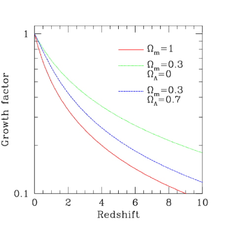
Figure 1: The redshift dependence of the linear growth mode of perturbations for a flat model with $\Omega_{m}=1$ (solid curve), for a flat $\Omega_{m}=0.3$ model with a cosmological constant (dashed curve) and for an $\Omega_{m}=0.3$ open model with vanishing cosmological constant (dotted curve).

The exact expression for the growing model of perturbations is given by

$$D_{+}(z)\,=\,{5\over 2}\,\Omega_{m}E(z)\,\int_{z}^{\infty}{1+z^{\prime}\over E(z^{\prime})^{3}}\,dz^{\prime}$$ (15)

(e.g., 1993ppc..book…..P ). I show in Figure 1 the redshift dependence of the linear growth factor for an Eds model and for two models with $\Omega_{m}=0.3$ both with and without a cosmological constant term to restore spatial flatness. Quite apparently, the EdS has the faster evolution, while the slowing down of the perturbation growth is more apparent for the open low–density model, the presence of cosmological constant providing an intermediate degree of evolution. A more pictorial view is provided in Figure 2, where we show the dark matter density fields for two different cosmologies and at different epochs, as obtained from N–body simulations. The two models, an EdS one and a flat low–density one with $\Omega_{m}=0.3$, have been tuned so as to have a similar appearance at $z=0$. This figure clearly shows that any observational probe of the degree of evolution of density perturbations would correspond to a sensitive probe of cosmological parameters. Such a cosmological test is conceptually different to those provided by the standard geometrical tests based on luminosity and angular–size distances.

As we shall discuss in the following, clusters of galaxies provide such a probe, since the evolution of their number density is directly related to the growth rate of perturbations.

Figure 2: The evolution of the cluster population from N–body simulations in two different cosmologies 2001Natur.409…39B . Left panels describe a flat, low–density model with $\Omega_{m}=0.3$ and $\Omega_{\Lambda}=0.7$ (L03); right panels are for an Einstein–de-Sitter model (EdS) with $\Omega_{m}=1$. Superimposed on the dark matter distribution, the yellow circles mark the positions of galaxy clusters with virial temperature $T>3$ keV, the size of the circles is proportional to temperature. Model parameters have been chosen to yield a comparable space density of clusters at the present time. Each snapshot is $250h^{-1}$ Mpc across and $75h^{-1}$ Mpc thick (comoving with the cosmic expansion).

2.3 The spherical top–hat collapse

A spherical perturbation at constant density represents the only case in which the evolution can be exactly computed. Although the assumptions on which this model is based are quite restrictive, nevertheless it serves as a very useful guideline to characterize the process of evolution and formation of virialized DM halos. This approach is based on treating the perturbation as a separate Friedmann–Lemaitre–Robertson–Walker (FLRW) universe, with the constraint of null velocity at the boundary of the perturbation. Here we will sketch the derivation in the case of $\Omega_{m}=1$ (e.g., 2002coec.book…..C , while an extension of this derivation to more general cosmologies can be found in 1996MNRAS.282..263E and 1996ApJ…469..480K , with useful fitting functions provided in 1998ApJ…495…80B .

Assuming null velocities at an initial time $t_{i}$ provides the relation $D_{+}(t_{i})=(3/5)\delta(t_{i})$, between the linear growth mode of the perturbation and the initial overdensity. The initial density parameter, which characterizes this separate Universe, is then $\Omega_{p}(t_{i})=\Omega(t_{i})(1+\delta_{i})$. Therefore, the condition for the perturbation to recollapse will be $\Omega_{p}(t_{i})>1$. If this condition is satisfied, then we can derive the density within the perturbation at the time $t_{m}$ of its maximum expansion (turn–around) as

$$\rho_{p}(t_{m})=\rho_{c}(t_{i})\Omega_{p}(t_{i})\left[{\Omega_{p}(t_{i})-1\over\Omega_{p}(t_{i})}\right]^{3}\,.$$ (16)

The time $t_{m}$ is given by the solution of the Friedmann equations for a closed Universe:

$$t_{m}={\pi\over 2H_{i}}{\Omega_{p}(t_{i})\over\left[\Omega_{p}(t_{i})-1\right]^{3/2}}=\left[{3\pi\over 32G\rho_{p}(t_{m})}\right]\,,$$ (17)

where $H_{i}$ is the Hubble parameter within the perturbation. At the same epoch $t_{m}$, the density of the general cosmic background is $\rho(t_{m})=(6\pi Gt_{m}^{2})^{-1}$. Therefore, the exact value for the perturbation overdensity at the turn–around is

$$\delta_{+}(t_{m})={\rho_{p}(t_{m})\over\rho(t_{m})}-1=\left({3\pi\over 4}\right)^{2}-1\simeq 4.6\,.$$ (18)

On the other hand, the linear–theory extrapolation to $t_{m}$ would give

$$\delta_{+}(t_{m})=\delta_{+}(t_{i})\left({t_{m}\over t_{i}}\right)^{2/3}={3\over 5}\left({3\pi\over 4}\right)^{2/3}\simeq 1.07\,.$$ (19)

This demonstrates that the linear–theory extrapolation significantly underestimates overdensities at the turn-around.

After reaching the maximum expansion, the perturbation then evolves by detaching from the general Hubble expansion and then recollapses, reaching virial equilibrium supported by the velocity dispersion of DM particles. This happens at the virialization time $t_{\rm vir}$, at which the perturbation meets by definition the virial condition $E=K+U=-K$, being $E$, $K$ and $U$ the total, the kinetic and the potential energy, respectively.

At the turn–around point, the perturbation has no kinetic energy, so that the total energy is

$$E_{m}=U=-{3\over 5}{GM^{2}\over R_{m}}\;\;,$$ (20)

where we have used the expression for the potential energy of a uniform spherical density field of radius $R_{m}$ and total mass $M$. In a similar manner, the total energy at the virialization is

$$E_{\rm vir}={U\over 2}=-{1\over 2}{3\over 5}{GM^{2}\over R_{\rm vir}}\,.$$ (21)

Therefore, the condition of energy conservation in a dissipationless collapse gives $R_{m}=2R_{\rm vir}$ for the relation between the radii at turn-around and at virial equilibrium. This allows us to compute the overdensity at $t_{\rm vir}$ as

$${\rho_{p}(t_{\rm vir})\over\rho(t_{\rm vir})}=\left({t_{\rm vir}\over t_{m}}\right)^{2}\left({R_{m}\over R_{\rm vir}}\right)^{3}{\rho_{p}(t_{m})\over\rho(t_{m})}=2^{2}2^{3}\left({3\pi\over 4}\right)^{2}=18\pi^{2}\simeq 178\,,$$ (22)

where we have accounted for both the compression of the perturbation density, due to its shrinking, and of the dilution of the background density as the Universe expands from $t_{m}$ to $t_{\rm vir}$. Eq.(22) shows why an overdensity of about 200 is usually considered as typical for a DM halo which has reached the condition of virial equilibrium. As for the extrapolation of linear–theory prediction, it would have given

$$\delta_{+}(t_{\rm vir})=\left({t_{\rm vir}\over t_{m}}\right)^{2/3}\delta_{+}(t_{m})\simeq 1.69\,.$$ (23)

The above equation shows the derivation of another fundamental number that will be used in what follows in order to characterize the mass function of virialized halos. It gives the overdensity that a perturbation in the initial density field must have for it to end up in a virialized structure. While the above derivation holds for an EdS Universe, it can be generalized to any generic cosmology. For $\Omega_{m}<1$ the increased expansion rate of the Universe causes a faster dilution of the cosmic density from $t_{m}$ to $t_{\rm vir}$ and, as a consequence, a larger value of the overdensity at virialization.

In the following, we will indicate with $\Delta_{\rm vir}$ the overdensity at virial equilibrium, computed with respect to the background density, and with $\Delta_{c}$ the same quantity expressed in units of the critical density $\rho_{c}$. As a reference, a flat low–density model with $\Omega_{m}=0.3$ has $\Delta_{c}\simeq 100$ and $\Delta_{\rm vir}\simeq 330$. Also, we will use in the following the notation $R_{N}$ to indicate the radius of a halo encompassing an average overdensity equal to $N\rho_{c}$, so that $M_{N}$ will denote the halo mass contained within that radius. As we shall see in the following, values often used in the literature are $N=200$, 500 and 2500.

3 The mass function

The mass function (MF) at redshift $z$, $n(M,z)$, is defined as the number density of virialized halos found at that redshift with mass in the range $[M,M+dM]$. In this section I will derive the MF expression following the approach originally devised by Press and Schechter PR74.1 (PS hereafter). After commenting on the limitations of this approach, I will discuss the accuracy with which improved derivations of the MF reproduce the “exact” predictions from N–body simulations.

3.1 The Press–Schechter mass function

The PS derivation of the MF is based on the assumption that the fraction of matter ending up in objects of a given mass $M$ can be found by looking at the portion of the initial (Lagrangian) density field, smoothed on the mass–scale $M$, lying at an overdensity exceeding a given critical threshold value, $\delta_{c}$. Under the assumption of Gaussian perturbations, the probability for the linearly–evolved smoothed field $\delta_{M}$ to exceed at redshift $z$ the critical density contrast $\delta_{c}$ reads

$$p_{>\delta_{c}}(M,z)={1\over\sqrt{2\pi}\sigma_{M}(z)}\int_{\delta_{c}}^{\infty}\exp\left(-{\delta_{M}^{2}\over 2\sigma_{M}(z)^{2}}\right)\,d\delta_{M}={1\over 2}{\rm erfc}\left({\delta_{c}\over\sqrt{2}\sigma_{M}(z)}\right)\,,$$ (24)

where ${\rm erfc}(x)$ is the complement error function and $\sigma_{M}(z)=\delta_{+}(z)\sigma_{M}$ is the variance at the mass scale $M$ linearly extrapolated at redshift $z$. Under the assumption of spherical collapse, the critical overdensity $\delta_{c}$ is given by the linear extrapolation of the overdensity at virial equilibrium, as derived in the previous section. In this case, it will be $\delta_{c}=\delta_{c}(z)$ with a weak dependence upon redshift and cosmological parameters, with $\delta_{c}\simeq 1.69$ independent of $z$ only in the case of an EdS cosmology. By definition, the above equation provides the fraction of unity volume, which ends up by redshift $z$ in objects with mass above $M$. Therefore, the fraction of Lagrangian volume in objects with mass in the range $[M,M+dM]$ is

$$dp_{>\delta_{c}}(M,z)=\left|{\partial p_{>\delta_{c}}(M,z)\over\partial M}\right|dM\,.$$ (25)

Since the probability of eq.(24) is a decreasing function of mass, the absolute value is required in order to have a positive–defined differential probability. Eq.(25) shows a fundamental limitation of the PS derivation of the MF. Indeed, we expect that, as we take the limit of arbitrarily small limiting mass, we should recover the whole mass content of the Universe. This is to say that, in the hierarchical clustering picture, all the mass is contained within halos of arbitrarily small mass. However, integrating eq.(25) over the whole mass range gives $\int_{0}^{\infty}dp_{>\delta_{c}}(M,z)=1/2$. This implies that the PS derivation of the mass function only accounts for half of the total mass at disposition. The basic reason for this is that, in this derivation, we give zero probability for a point with $\delta_{M}<\delta_{c}$, for a given filtering mass scale $M$, to have $\delta_{M^{\prime}}>\delta_{c}$ for some larger filtering scale $M^{\prime}>M$. This means that the PS approach neglects the possibility for that point to end up in a collapsed halo of larger mass. A more rigorous derivation of the mass function, which is based on the excursion–set formalism 1991ApJ…379..440B , correctly accounts for the missing factor 2, at least for the particular choice of a sharp–$k$ filter (i.e., a top–hat window function in Fourier space).

Since eq.(25) provides the fraction of volume in objects of a given mass, the number density of such objects will be obtained after dividing it by the volume, $V_{M}=M/\bar{\rho}$, occupied by each object. Therefore, after accounting for the missing factor 2, the expression for the mass function reads

$${dn(M,z)\over dM} = {2\over V_{M}}{\partial p_{>\delta_{c}}(M,z)\over\partial M}$$ (26)

$$= \sqrt{2\over\pi}{\bar{\rho}\over M^{2}}{\delta_{c}\over\sigma_{M}(z)}\left|{d\log\sigma_{M}(z)\over d\log M}\right|\exp\left(-{\delta_{c}^{2}\over 2\sigma_{M}(z)^{2}}\right)\,.$$

This is the expression for the PS mass function. Although we will present below a more accurate expressions for the MF, this equation already demonstrates the reason for which the mass function of galaxy clusters is a powerful probe of cosmological models. Cosmological parameters enter in eq.(26) through the mass variance $\sigma_{M}$, which depends on the power spectrum and on the cosmological density parameters, through the linear perturbation growth factor, and, to a lesser degree, through the critical density contrast $\delta_{c}$. Taking this expression in the limit of massive objects (i.e., rich galaxy clusters), the MF shape is dominated by the exponential tail. This implies that the MF becomes exponentially sensitive to the choice of the cosmological parameters. In other words, a reliable observational determination of the MF of rich clusters would allow us to place tight constraints on cosmological parameters.

3.2 Extensions of the PS approach and N–body tests

Following JE01.1 , an alternative way of recasting the mass function is

$$f(\sigma_{M},z)={M\over\bar{\rho}}{dn(M,z)\over d\ln\sigma_{M}^{-1}}\,.$$ (27)

In this way, the PS expression is recovered by setting

$$f(\sigma_{M},z)=\sqrt{2\over\pi}{\delta_{c}\over\sigma_{M}}\exp\left(-{\delta_{c}^{2}\over 2\sigma_{M}^{2}}\right)$$ (28)

Despite its subtle simplicity (e.g., 1998FCPh…19..157M ), the PS MF has served for more than a decade as a guide to constrain cosmological parameters from the mass distribution of galaxy clusters. Only with the advent of a new generation of N–body simulations, which are able to cover a very large dynamical range, have significant deviations of the PS expression from the exact numerical description been noticed (e.g., 1998MNRAS.301…81G ; 1999MNRAS.307..949G ; JE01.1 ; 2002ApJ…573….7E ; 2005Natur.435..629S ; 2005astro.ph..6395W ). Such deviations have been usually interpreted in terms of corrections to the PS approach.

Incorporating the effect of non–spherical collapse, the PS expression has been generalized SH99.1 to

$$f(\sigma_{M},z)=\sqrt{2a\over\pi}C\left[1+\left({\sigma_{M}^{2}\over a\delta_{c}^{2}}\right)^{q}\right]{\delta_{c}\over\sigma_{M}}\exp\left(-{a\delta_{c}^{2}\over 2\sigma_{M}^{2}}\right)\,.$$ (29)

These authors also compared this expression with results from N–body simulations, in which the mass of the clusters were estimated with a spherical overdensity (SO) algorithm, by computing the mass within the radius encompassing a mean overdensity equal to the virial one. As a result, they found the best–fitting values $a=0.707$, $q=0.3$, with the normalization constant $C=0.3222$ obtained from the normalization requirement $\int_{0}^{\infty}f(\sigma_{M})d\nu=1$ (note that the PS expression is recovered for $a=1$, $q=0$ and $C=1/2$; see also 2002MNRAS.329…61S ).

Jenkins et al. JE01.1 proposed an alternative expression for the mass function:

$$f(\sigma_{M},z)=0.315\exp(-|\ln\sigma_{M}^{-1}+0.61|^{3.8})\,,$$ (30)

which has been obtained as the best fit to the results of a combination of different simulations, covering a wide dynamical range. More recently, Springel et al. 2005Natur.435..629S used the largest available single N–body simulation to verify in detail the accuracy of eq.(30). The result of this comparison, which is reported in Figure 3, demonstrates that this mass function reproduces remarkably well numerical results over a wide range of sampled halo masses and redshifts, thereby representing a substantial improvement with respect to the PS mass function. The accuracy of eq.(30) in reproducing results of numerical experiments has been also discussed in 2002ApJ…573….7E , where it is also pointed out the role of different algorithms to identify clusters and to estimate their mass in simulations, in 2002ApJS..143..241W , where the universality of this expression for a generic cosmology is discussed, and in 2005astro.ph..6395W , where the widest dynamical range to date has been samples by combining a series of N–body simulations.

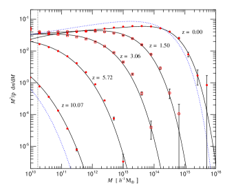
Figure 3: Left panel: the mass function of DM halos (dots with errorbars) identified at different redshifts in the Millenniun Run 2005Natur.435..629S , compared to the predictions of the mass function by JE01.1 and by PR74.1 . The two model mass functions are plotted with solid and dotted curves, respectively. Right panel: the relative standard deviation of $\sigma_{8}$ as a function of the sample size 2002ApJS..143..241W from the cumulative mass function above two different mass limits. The solid lines indicate the width of the distribution when including the clustering of clusters.

In practical applications, the observational mass function of clusters is usually determined over about one decade in mass. Therefore, it probes the power spectrum over a relatively narrow dynamical range, and does not provide strong constraints on the shape of the power spectrum. Using only the number density of nearby clusters of a given mass $M$, one can constrain the amplitude of the density perturbation at the physical scale $R\propto(M/\Omega_{m}\rho_{crit})^{1/3}$ which contains this mass. Since such a scale depends both on $M$ and on $\Omega_{m}$, the mass function of nearby ($z\raise-2.0pt\hbox{\hbox to0.0pt{\hbox{$\sim$}\hss}\raise 5.0pt\hbox{$<$}\ }0.1$) clusters is only able to constrain a relation between $\sigma_{8}$ and $\Omega_{m}$. In the left panel of Figure 4 we show that, for a fixed value of the observed cluster mass function, the implied value of $\sigma_{8}$ from eq.(29) increases as the density parameter decreases. Determinations of the cluster mass function in the local Universe using a variety of samples and methods indicate that $\sigma_{8}\Omega_{m}^{\alpha}\,=\,0.4-0.6$, where $\alpha\simeq 0.4-0.6$, almost independent of the presence of a cosmological constant term providing spatial flatness. As for the evolution with redshift, the growth rate of the density perturbations depends primarily on $\Omega_{m}$ and, to a lesser extent, on $\Omega_{\Lambda}$, at least out to $z\sim 1$, where the evolution of the cluster population is currently studied. Therefore, following the evolution of the cluster space density over a large redshift baseline, one can break the degeneracy between $\sigma_{8}$ and $\Omega_{m}$. This is shown in a pictorial way in Figure 2 and quantified in the right panel of Figure 4: models with different values of $\Omega_{m}$, which are normalized to yield a comparable number density of nearby clusters, predict cumulative mass functions that progressively differ by up to orders of magnitude at increasing redshifts.

Although eq.(30) provides a very accurate and flexible tool to constrain the parameter space of cosmological models using the mass function of collapsed halos, nevertheless a further source of uncertainty may arise from the effect of cosmic variance. Fluctuations modes, with wavelength exceeding the size of the volumes sampled by observations, induces appreciable changes in the number counts of halos of a given mass. This effect has been thoroughly discussed in 2003ApJ…584..702H ; 2002ApJS..143..241W . In the right panel Figure 3 (from 2002ApJS..143..241W ) I report the relative variation of the power spectrum normalization, $\sigma_{8}$, induced by cosmic variance, as a function of the sample size, for halos having two different mass limits. As expected, the variance decreases with the sample size (fluctuations on larger scales have a smaller effect), while it increases with the halo mass (the distribution of rarer objects suffer for a more pronounced large–scale modulation). This result demonstrates that a precision calibration of cosmological parameters requires properly accounting for the effect of cosmic variance.

            

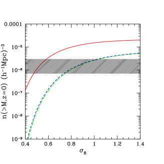
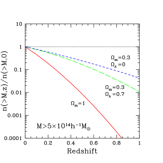
Figure 4: The sensitivity of the cluster mass function to cosmological models 2002ARA&A..40..539R . Left panel: The cumulative mass function at $z=0$ for $M>5\times 10^{14}h^{-1}M_{\odot}$ for three cosmologies, as a function of $\sigma_{8}$, with shape parameter $\Gamma=0.2$; solid line: $\Omega_{m}=1$; short–dashed line: $\Omega_{m}=0.3$, $\Omega_{\Lambda}=0.7$; long–dashed line: $\Omega_{m}=0.3$, $\Omega_{\Lambda}=0$. The shaded area indicates the observational uncertainty in the determination of the local cluster space density. Right panel: Evolution of $n(>\!M,z)$ for the same cosmologies and the same mass–limit, with $\sigma_{8}=0.5$ for the $\Omega_{m}=1$ case and $\sigma_{8}=0.8$ for the low–density models.

4 Building a cluster sample

4.1 Identification in the optical / near IR band

Abell Ab58 provided the first extensive, statistically complete sample of galaxy clusters, later extended to the Southern hemisphere ACO89 . Based on purely visual inspection, clusters were identified as enhancements in the galaxy surface density and were characterized by their richness and estimated distance. The Abell catalog has been for decades the prime source for detailed studies of individual clusters and for characterizing the large scale distribution of matter in the nearby Universe. Several variations of the Abell criteria defining clusters were used in an automated and objective fashion when digitized optical plates became available (e.g., 1992MNRAS.258….1L ; 1997MNRAS.289..263D ). Deep optical plates were used successfully to search for more distant clusters, out to $z\simeq 0.9$, with purely visual techniques (e.g., 1986ApJ…306…30G ; 1991MNRAS.249..606C ). These searches for distant clusters became much more effective with the advent of CCD imaging. Postman et al. 1996AJ….111..615P were the first to carry out a V&I-band survey over 5 deg² (the Palomar Distant Cluster Survey, PDCS). This technique enhances the contrast of galaxy overdensity at a given position, utilizing prior knowledge of the luminosity profile typical of galaxy clusters. Dalcanton 1996ApJ…466…92D proposed another method of optical selection of clusters, in which drift scan imaging data from relatively small telescopes is used to detect clusters as positive surface brightness fluctuations in the background sky. Gonzalez et al. 2001ApJS..137..117G applied a technique based on surface brightness fluctuations from drift scan imaging data to build a sample of $\sim\!1000$ cluster candidates over 130 deg².

A common feature of all these methods of cluster identification is that they classify clusters according to definitions of richness, which generally have a loose relation with the actual cluster mass. This represents a serious limitation for any cosmological application, which requires the observable, on which the cluster selection is based, to be a reliable proxy of the cluster mass.

An improved definition of richness, based on the amplitude of the galaxy–cluster cross–correlation function, has been applied 2005ApJS..157….1G to clusters identified in a large area survey in $R$ and $z$ bands (the Red Sequence Cluster Survey). This survey, whose optical and X–ray follow–up, is currently underway, promises to unveil a fairly large number of clusters out to $z\sim 1.5$.

By increasing the number of observed passbands and using red colors one can increase the contrast with which clusters are seen in color space. In this way, one can increase the efficiency of cluster selection also at high redshift (e.g., 2002AJ….123..619S ; 2005ApJS..157….1G ; 2005ApJ…634L.129S ) and the accuracy of their estimated redshifts through spectro–photometric techniques. In this way, Miller et al. 2005AJ….130..968M designed a cluster–finding algorithm which makes full use of information of both position and color space to detect clusters of galaxies from the SDSS. They were able to identify about 750 clusters out to $z\raise-2.0pt\hbox{\hbox to0.0pt{\hbox{$\sim$}\hss}\raise 5.0pt\hbox{$<$}\ }0.2$, and assessed the degree of completeness by resorting to a comparison with mock SDSS surveys extracted from large N–body simulations. Once completed, the search of clusters over the entire SDSS sample will provide about 2500 nearby and medium–distant objects. At the same time the next generation of wide field ($>\!100$ deg²) deep multicolor surveys in the optical and especially the near-infrared will powerfully enhance the search for distant clusters, out to $z\raise-2.0pt\hbox{\hbox to0.0pt{\hbox{$\sim$}\hss}\raise 5.0pt\hbox{$>$}\ }1$.

4.2 Identification in the X–ray band

Already from the first pioneering attempts to map the X–ray sky (1972ApJ…178..281G , see 2002ARA&A..40..539R for a historical review), clusters were associated with extended sources, whose dominant emission mechanism was recognized to be thermal bremsstrahlung from optically thin plasma at a temperature of several keV 1966ApJ…146..955F ; 1971Natur.231..437C . The all–sky survey conducted by the the HEAO-1 X-ray Observatory was the first to provide a flux–limited sample of X–ray identified clusters, for which both the flux number counts and the X–ray luminosity function have been computed for the first time 1982ApJ…253..485P . However, it is only thanks to the much improved sensitivity of the Einstein Observatory 1979ApJ…230..540G that X-ray surveys were recognized as an efficient means of constructing samples of galaxy clusters out to cosmologically interesting redshifts.

First, the X-ray selection has the advantage of revealing physically-bound systems, because diffuse emission from a hot ICM is the direct manifestation of the existence of a potential-well within which the gas is in dynamical equilibrium with the cool baryonic matter (galaxies) and the dark matter. Second, the X-ray luminosity is well correlated with the cluster mass (see Figure 11). Third, the X-ray emissivity is proportional to the square of the gas density, hence cluster emission is more concentrated than the optical bidimensional galaxy distribution. In combination with the relatively low surface density of X-ray sources, this property makes clusters high contrast objects in the X-ray sky, and alleviates problems due to projection effects that affect optical selection. Finally, an inherent fundamental advantage of X-ray selection is the ability to define flux-limited samples with well-understood selection functions. This leads to a simple evaluation of the survey volume and therefore to a straightforward computation of space densities. Nonetheless, there are some important caveats described below. Pioneering work in this field 1990ApJ…356L..35G ; 1992ApJ…386..408H was based on the Einstein Observatory Extended Medium Sensitivity Survey (EMSS). The EMSS survey covered over 700 square degrees and lead to the construction of a flux-limited sample of 93 clusters out to $z=0.58$, allowing the cosmological evolution of clusters to be investigated.

The ROSAT satellite, launched in 1990, allowed a significant step forward in X-ray surveys of clusters. The ROSAT All-Sky Survey (RASS, 1993Sci…260.1769T ) was the first X-ray imaging mission to cover the entire sky, thus paving the way to large contiguous-area surveys of X-ray selected nearby clusters. In the northern hemisphere, the largest compilations with virtually complete optical identification include, the Bright Cluster Sample (BCS, 2000MNRAS.318..333E ), and the Northern ROSAT All Sky Survey (NORAS, 2000ApJS..129..435B ). In the southern hemisphere, the ROSAT-ESO flux limited X-ray (REFLEX) cluster survey 2004A&A…425..367B has completed the identification of 452 clusters, the largest, homogeneous compilation to date. The Massive Cluster Survey (MACS, 2001ApJ…553..668E ) is aimed at targeting the most luminous systems at $z>0.3$ which can be identified in the RASS at the faintest flux levels. The deepest area in the RASS, the North Ecliptic Pole (NEP, 2001ApJ…553L.109H ) which ROSAT scanned repeatedly during its All-Sky survey, was used to carry out a complete optical identification of X-ray sources over a 81 deg² region. This study yielded 64 clusters out to redshift $z=0.81$.

In total, surveys covering more than $10^{4}$ deg² have yielded over 1000 clusters, out to redshift $z\simeq 0.5$. A large fraction of these are new discoveries, whereas approximately one third are identified as clusters in the Abell or Zwicky catalogs. For the homogeneity of their selection and the high degree of completeness of their spectroscopic identifications, these samples are now the basis for a large number of follow-up investigations and cosmological studies.

Besides the all-sky surveys, the ROSAT-PSPC archival pointed observations were intensively used for serendipitous searches of distant clusters. These projects, which are now completed, include: the RIXOS survey 1995Natur.377…39C , the ROSAT Deep Cluster Survey (RDCS, 1998ApJ…492L..21R ; 2002ARA&A..40..539R ), the Serendipitous High-Redshift Archival ROSAT Cluster survey (SHARC, 1997ApJ…488L..83B , the Wide Angle ROSAT Pointed X-ray Survey of clusters (WARPS, 2002ApJS..140..265P ), the 160 deg² large area survey 2003ApJ…594..154M , the ROSAT Optical X-ray Survey (ROXS, 2001ApJ…552L..93D ). ROSAT-HRI pointed observations have also been used to search for distant clusters in the Brera Multi-scale Wavelet catalog (BMW, 2004A&A…428…21M ).

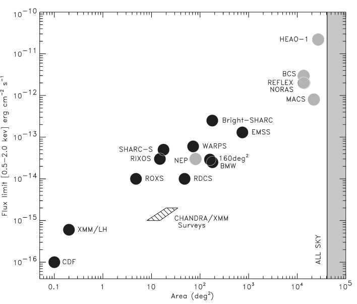
Figure 5: Solid angles and flux limits of X-ray cluster surveys carried out over the last two decades. Dark filled circles represent serendipitous surveys constructed from a collection of pointed observations. Light shaded circles represent surveys covering contiguous areas. The hatched region is a predicted locus of current serendipitous surveys with Chandra and Newton-XMM. From 2002ARA&A..40..539R .

In Figure 5, we give an overview of the flux limits and surveyed areas of all major cluster surveys carried out over the last two decades. RASS-based surveys have the advantage of covering contiguous regions of the sky so that the clustering properties of clusters (e.g., 2001A&A…368…86S ) can be investigated. They also have the ability to unveil rare, massive systems albeit over a limited redshift and X-ray luminosity range. Serendipitous surveys which are at least a factor of ten deeper but cover only a few hundreds square degrees, provide complementary information on lower luminosities, more common systems and are well suited for studying cluster evolution on a larger redshift baseline.

A number of systematic studies have been carried out to compare the nature of clusters identified with the optical and the X–ray technique (e.g., Dona02 ; Basil04 ; Plio05 ). The general conclusion of these studies is that optically selected clusters are on average underluminous in the X-ray band. This suggests that optical selection tends to pick up objects which have not yet reached a high enough density to make the ICM lighting up in X–rays.

In order for a survey to be used for cosmological applications, one needs to know not only how many clusters it contains, but also the volume within which each of them is found. In other words, one needs to define the selection function of the survey, which depends on the survey strategy and on the details of the adopted cluster finding algorithm (see 2002ARA&A..40..539R , for a review). An essential ingredient for the evaluation of the selection function of X-ray surveys is the computation of the sky coverage: the effective area covered by the survey as a function of flux. In general, the exposure time, as well as the background and the PSF are not uniform across the field of view of X-ray telescopes, which introduces vignetting and a degradation of the PSF at increasing off-axis angles. As a result, the sensitivity to source detection varies significantly across the survey area so that only bright sources can be detected over the entire solid angle of the survey, whereas at faint fluxes the effective area decreases. An example of survey sky coverage is given in the left panel of Figure 6. By covering different solid angles at varying fluxes, these surveys probe different volumes at increasing redshift and therefore different ranges in X-ray luminosities at varying redshifts.

Once the survey flux–limit and the sky coverage are defined one can compute the maximum search volume, $V_{max}$, within which a cluster of a given luminosity is found in that survey:

$$V_{max}=\int_{0}^{z_{max}}S[f(L,z)]\left({d_{L}(z)\over 1+z}\right)^{2}{c\,dz\over H(z)}\,.$$ (31)

Here $S(f)$ is the survey sky coverage, which depends on the flux $f=L/(4\pi d_{L}^{2})$, $d_{L}(z)$ is the luminosity distance, and $H(z)$ is the Hubble constant at $z$. We define $z_{max}$ as the maximum redshift out to which the flux of an object of luminosity $L$ lies above the flux limit. The corresponding survey volumes are shown in the right panel of Figure 6.

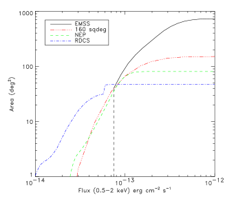
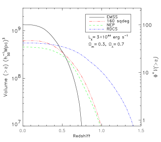
Figure 6: Left panel: sky coverage as a function of X-ray flux of several serendipitous surveys. Right panel: corresponding search volumes, $V(>z)$, for a cluster of given $X$-ray luminosity ($L_{X}=3\times 10^{44}\,[0.5-2\,\rm{keV}]\simeq L_{X}^{*}$). From 2002ARA&A..40..539R .

Once again, I emphasize that one of the main advantages of the X–ray selection lies in the fact that the survey selection function can be precisely computed, thus allowing reliable comparisons between the observed and the predicted evolution of the cluster population.

4.3 Identification through the SZ effect

The Sunyaev–Zeldovich (SZ) effect 1972CoASP…4..173S allows to observe galaxy clusters by measuring the distortion of the CMB spectrum owing to the hot ICM. This method does not depend on redshift and provides in principle a reliable estimate of cluster masses. For these reasons, it is now considered as one of the most powerful means to find distant clusters in the years to come. For a detailed discussion of the SZ technique for cluster identification and for the ongoing and future surveys, I refer to the lectures by Mark Birkinshaw and to the reviews in 1999PhR…310…97B ; 2002ARA&A..40..643C . For the purpose of the present discussion, I show in the left panel of Figure 7 a comparison between the limiting mass as a function of redshift, expected for a X–ray and for a SZ cluster survey (from 2001ApJ…553..545H ). While the standard flux dimming with the luminosity distance, $f_{X}\propto d_{L}^{2}(z)$, causes the limiting mass to quickly increase with distance for the X–ray selection, this limiting mass has a much less sensitive dependence on redshift for the SZ selection. This is the reason why SZ surveys are generally considered as essentially providing mass–limited cluster samples.

It has been recently pointed out 2005ApJ…623L..63M that the integrated SZ flux–decrement has a very tight correlation with the total cluster mass (see also 2005MNRAS.356.1477D ). This fact, joined with the redshift–independence of the SZ selection, makes the SZ identification a promising route toward precision cosmology with galaxy clusters.

A potential problem with the SZ identification of clusters resides in the possible contamination of the signal from foreground/background structures. Diffuse gas, residing in large–scale filaments, are likely to provide a negligible contamination, as a consequence of the comparatively low density and temperature which characterize such structures. However, small halos, which are expected to be present in large number, contain gas at the virial overdensity. Since they are not resolved in current SZ observations, their integrated contribution may provide a significant contamination. Using cosmological hydro-dynamical simulations, White et al. 2002ApJ…579…16W have created SZ sky maps with the aim of correlating the SZ signal seen in projection with the actual mass of clusters.The result of this test is shown in the right panel of Fig. 7. The upper panel shows the relation between the integrated SZ signal contributed only from the gas within $0.5R_{200}$ and $M_{200}$, while the lower panel is when using the actual Compton–$y$ parameter measured from the projected maps. Quite apparently, the scatter in the relation is significantly increased in projection. Part of the scatter is due to the different redshifts at which clusters seen in projection are placed. This contribution to the scatter can be removed once redshifts of clusters are known from follow–up optical observations. However, a significant contribution to the overall scatter is contributed by cluster asphericity and by contamination from fore/background structures. This highlights the relevance of keeping this scatter under control for a full exploitation of the SZ signal as a tracer of the cluster mass.

Figure 7: Left panel: limiting cluster virial mass for detection in an X–ray and in a SZ survey (from 2001ApJ…553..545H ). Each pair of curves show the results for two $\Omega_{m}=0.3$ cosmologies, having $w=-1$ and $w=-0.5$ for the DE equation of state. Right panel: the relation between the Comptonization parameter and $M_{200}$, from 2002ApJ…579…16W . The upper panel shows the decrement contributed from the gas within $0.5R_{200}$. The lower panel indicates the signal from noise–free maps projected on the light cone.

5 Methods to estimate cluster masses

5.1 The hydrostatic equilibrium

The condition of hydrostatic equilibrium determines the balance between the pressure force and the gravitational force: $\nabla P_{\rm gas}=-\rho_{\rm gas}\nabla\phi$, where $P_{\rm gas}$ and $\rho_{\rm gas}$ are the gas pressure and density, respectively, while $\phi$ is the underlying gravitational potential. Under the assumption of a spherically symmetric gas distribution, the above equations read:

$${dP_{\rm gas}\over dr}=-\rho_{\rm gas}{d\phi\over dr}=-\rho_{\rm gas}{GM(<r)\over r^{2}}\,,$$ (32)

where $r$ is the radial coordinate (clustercentric distance) and $M(<r)$ is the total mass contained within $r$. Using the equation of state of ideal gas to relate pressure to gas density and temperature, the mass is then given by

$$M(<r)=-{r\over G}{k_{B}T\over\mu m_{p}}\left({d\ln\rho_{\rm gas}\over d\ln r}+{d\ln T\over d\ln r}\right)\,,$$ (33)

where $\mu$ is the mean molecular weight of the gas ($\mu\simeq 0.59$ for primordial composition) and $m_{p}$ is the proton mass. An often used mass estimator is based on assuming the $\beta$–model for the gas density profile,

$$\rho_{\rm gas}(r)={\rho_{0}\over\left[1+(r/r_{c})^{2}\right]^{3\beta/2}}$$ (34)

1976A&A….49..137C . In the above equation, $r_{c}$ is the core radius, while $\beta$ is the ratio between the kinetic energy of any tracer of the gravitational potential (e.g. galaxies) and the thermal energy of the gas, $\beta=\mu m_{p}\sigma_{v}^{2}/(k_{B}T)$ ($\sigma_{v}$: one–dimensional velocity dispersion). By further assuming a polytropic equation of state, $\rho_{\rm gas}\propto P_{\rm gas}^{\gamma}$ ($\gamma$: polytropic index), eq.(33) becomes

$$M(<r)\simeq 1.11\times 10^{14}\beta\gamma{T(r)\over{\rm keV}}{r\over\,h^{-1}{\rm Mpc}}{(r/r_{c})^{2}\over 1+(r/r_{c})^{2}}\,h^{-1}M_{\odot}\,,$$ (35)

where $T(r)$ is the temperature at the radius $r$. In its original derivation, the $\beta$–model was aimed at representing the distribution of isothermal gas sitting in hydrostatic equilibrium within a King–like potential. The corresponding mass estimator is recovered from eq.(35) by setting $\gamma=1$ and replacing $T(r)$ with the global ICM temperature, $T_{0}$. In the absence of accurately resolved temperature profiles from X–ray observations, eq.(35) has been used to estimate cluster masses both in its isothermal (e.g., RE02.1 ) and in its polytropic form (e.g., 2000ApJ…532..694N ; 2001A&A…368..749F ; 2002A&A…391..841E ).

Thanks to the much improved sensitivity of the Chandra and XMM–Newton X–ray observatories, temperature profiles are now resolved with high enough accuracy to allow the application of more general methods of mass estimation, not necessarily bound to the assumptions of $\beta$–model and of an overall polytropic form for the equation of state (e.g., 2001MNRAS.328L..37A ; 2002A&A…391..841E ; 2005A&A…441..893A ; 2005astro.ph..7092V ).

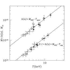
Figure 8: The mass-temperature relation for nearby clusters (from 2005A&A…441..893A ) and for distant clusters (from 2005ApJ…633..781K ), based on a combination of Chandra and XMM–Newton data.

An alternative way of recasting the isothermal version of eq.(35) between temperature and mass is based on expressing the mass according to the virial theorem as $M_{\rm vir}=\sigma_{v}^{2}R_{\rm vir}/G$, so that

$$k_{B}T={1.38\over\beta}\left({M_{\rm vir}\over 10^{15}\,h^{-1}M_{\odot}}\right)^{3/2}\left[\Omega_{m}\Delta_{\rm vir}(z)\right]^{1/3}(1+z)\,{\rm keV}\,.$$ (36)

This expression, originally introduced in 1996MNRAS.282..263E , has been sometimes used to express the $M$–$T$ relation as obtained from hydrodynamical simulations of galaxy clusters (e.g., 1998ApJ…495…80B ; 2002MNRAS.336..409B ).

It is clear that the two crucial assumptions underlying any mass measurements based on the ICM temperature concerns the existence of hydrostatic equilibrium and of spherical symmetry. While effects of non–spherical geometry can be averaged out by performing the analysis over a large enough number of clusters, the former can lead to systematic biases in the mass estimates (e.g., 2005ApJ…618L…1R ) and references therein). So far, ICM temperature measurements have been based on fits of the observed X–ray spectra of clusters to plasma models, which are dominated at high temperatures by thermal bremsstrahlung. However, local deviations from isothermality, e.g. due to the presence of merging cold gas clumps, can bias the spectroscopic temperature with respect to the actual electron temperature (e.g., 2001ApJ…546..100M ; 2004MNRAS.354…10M ; 2005astro.ph..4098V ). This bias directly translates into a comparable bias in the mass estimate through hydrostatic equilibrium (see Section 7, below).

5.2 The dynamics of member galaxies

From a historical point of view, the dynamics traced by member galaxies, has been the first method applied to measure masses of galaxy clusters 1936ApJ….83…23S ; 1937ApJ….86..217Z . Under the assumption of virial equilibrium, the mass of the cluster can be estimated by knowing position and redshift for a high enough number of member galaxies:

$$M={\pi\over 2}{3\sigma_{v}^{2}R_{V}\over G}$$ (37)

(e.g., 1960ApJ…132..286L ), where the first factor accounts for the geometry of projection, $\sigma_{r}$ is the line-of-sight velocity dispersion and $R_{V}$ is the virialization radius, which depends on the positions of the galaxies with measured redshifts and recognized as true cluster members:

$$R_{V}=N^{2}\left(\sum_{i>j}r_{ij}^{-1}\right)^{-1}\,,$$ (38)

where $N$ is the total number of galaxies, and $r_{ij}$ the projected separation between the $i$-th and $j$-th galaxies. This method has been extensively applied to measure masses for statistical samples of both nearby (e.g., 1993ApJ…411L..13B ; 1998ApJ…505…74G ; 2003ApJ…585..205B ; 2003AJ….126.2152R ; 2005A&A…433..431P ) and distant (e.g., 1997ApJ…476L…7C ; 2001ApJ…548…79G ) clusters.

Besides the assumption of virial equilibrium, which may be fulfilled to different degrees by different populations of galaxies (e.g., late vs. early type), a crucial aspect in the application of the dynamical mass estimator concerns the rejection of interlopers, i.e. of back/foreground galaxies which lie along the line-of-sight of the cluster without belonging to it. A spurious inclusion of non–member galaxies in the analysis leads in general to an overestimate of the velocity dispersion and, therefore, of the resulting mass. A number of algorithms have been developed for interlopers rejection, whose reliability must be judged on a case-by-case basis (e.g., 1993ApJ…404…38G ; 1997MNRAS.287..817V ). A further potential problem of this analysis concerns the possibility of realizing a uniform sampling of the cluster potential using galaxies with measured redshifts. For instance, the technical difficulty of packing slits or fibers in optical spectroscopic observations may lead to an undersampling of the cluster central regions. In turn, this leads to an overestimate of $R_{V}$ and, again, of the collapsed mass.

Tests of the accuracy of mess estimates based on the dynamical virial method have been performed by using hydrodynamical simulations of galaxy clusters, in which galaxies are identified from gas cooling and star formation (1996ApJ…472..460F ; Biviano06 ). For instance, Biviano06 have shown that galaxies identified in the simulations are fair tracers of the underlying dynamics, with no systematic bias in the estimate of cluster masses, although a rather large scatter between true and recovered masses is induced mostly by projection effects.

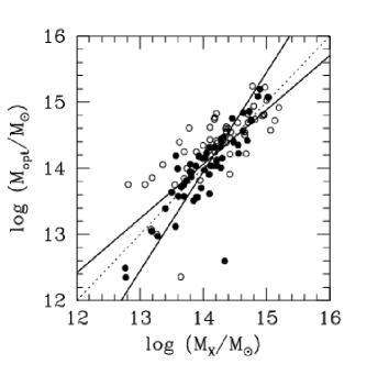
Figure 9: The relation between dynamical optical masses and masses derived from the X–ray temperature by assuming hydrostatic equilibrium (from 1998ApJ…505…74G , left panel, and from 2005A&A…433..431P , right panel, based on SDSS spectroscopic data).

Quite reassuringly, despite all the assumptions and possible systematics affecting both dynamical optical and X–ray mass estimates, these two methods provide in general fairly consistent results for both nearby (e.g., 1998ApJ…505…74G ; 2005A&A…433..431P ) and distant (e.g., 1999ApJ…517..587L ) clusters. Two examples of such comparisons are shown in Figure 9. In the left panel, we report the comparison between X–ray and optical dynamical masses 1998ApJ…505…74G . This plot shows a reasonable agreement among the two mass estimates, although with some scatter. The right panel reports the comparison presented in 2005A&A…433..431P . In this plot, the triangles indicates the cluster with clear evidences of complex dynamics. Quite interestingly, the agreement between the two mass estimates is acceptable, with a few outliers which are generally identified with non–relaxed clusters.

5.3 The self–similar scaling

The simplest model to explain the physics of the ICM is based on the assumption that gravity only determines the thermodynamical properties of the hot diffuse gas 1986MNRAS.222..323K . Since gravity does not have a preferred scale, we expect clusters of different sizes to be the scaled version of each other as long as gravity only determines the ICM evolution and there are no preferred scales in the underlying cosmological model. This is the reason why the ICM model based on the effect of gravity only is said to be self-similar.

If we define $M_{\Delta_{c}}$ as the mass contained within the radius $R_{\Delta_{c}}$, encompassing a mean density $\Delta_{c}$ times the critical density, then $M_{\Delta_{c}}\propto\rho_{c}(z)\Delta_{c}R_{\Delta_{c}}^{3}$. Here $\rho_{c}(z)$ is the critical density of the universe which scales with redshift as $\rho_{c}(z)=\rho_{c,0}E^{2}(z)$, where $E(z)$ is given by eq.(12). On the other hand, the cluster size $R$ scales with $z$ and $M_{\Delta_{c}}$ as $R\propto M^{1/3}E^{-2/3}(z)$. Therefore, assuming hydrostatic equilibrium, the cluster mass scales with the temperature $T$ as

$$M_{\Delta_{c}}\,\propto\,T^{3/2}E^{-1}(z)\,.$$ (39)

If $\rho_{\rm gas}$ is the gas density, the corresponding X–ray luminosity for pure thermal bremsstrahlung emission is

$$L_{X}\,=\,\int_{V}\left({\rho_{\rm gas}\over\mu m_{p}}\right)^{2}\Lambda(T)\,dV\,,$$ (40)

where $\Lambda(T)\propto T^{1/2}$. Further assuming that the gas distribution traces the dark matter distribution, $\rho_{\rm gas}(r)\propto\rho_{DM}(r)$, then

$$L_{X}\,\propto\,M_{\Delta_{c}}\rho_{c}T^{1/2}\,\propto\,T^{2}E(z)\,.$$ (41)

As for the CMB intensity decrement due to the thermal SZ effect we have

$$\Delta S\,\propto\,\int y(\theta){\rm d}\Omega\,\propto\,d_{A}^{-2}\int Tn_{e}{\rm d}^{3}r\propto d_{A}^{-2}T^{5/2}E^{-1}(z)\,,$$ (42)

where $y$ is the Comptonization parameter, $d_{A}$ is the angular size distance and $n_{e}$ is the electron number density. We can also write $\Delta S$ in a different way to get the explicit dependence on $y_{0}$:

$$\Delta S\,\propto\,y_{0}d_{A}^{-2}\int{\rm d}\Omega\propto y_{0}d_{A}^{-2}M^{2/3}E^{-4/3}(z)\,\propto\,y_{0}d_{A}^{-2}TE^{-2}(z)\,.$$ (43)

In this way, we obtain the following scalings for the central value of the Comptonization parameter:

$$y_{0}\,\propto\,T^{3/2}E(z)\,\propto\,L_{X}^{3/4}E^{1/4}(z)\,.$$ (44)

Eqs.(39), (41) and (44) are unique predictions for the scaling relations among ICM physical quantities and, in principle, they provide a way to relate the cluster masses to observables at different redshifts. As we shall discuss in the following, deviations with respect to these relations witness the presence of more complex physical processes, beyond gravitational dynamics only, which affect the thermodynamical properties of the diffuse baryons and, therefore, the relation between observables and cluster masses.

5.4 Phenomenological scaling relations

Using the X–ray luminosity

The relation between X–ray luminosity and temperature of nearby clusters is considered as one of the most robust observational facts against the self–similar model of the ICM. A number of observational determinations now exist, pointing toward a relation $L_{X}\propto T^{\alpha}$, with $\alpha\simeq 2.5$–3 (e.g., 2000ApJ…538…65X ), possibly flattening towards the self–similar scaling only for the very hot systems with $T\raise-2.0pt\hbox{\hbox to0.0pt{\hbox{$\sim$}\hss}\raise 5.0pt\hbox{$>$}\ }10$ keV Allen98 . While in general the scatter around the best–fitting relation is non negligible, it has been shown to be significantly reduced after excising the contribution to the luminosity from the cluster cooling regions 1998ApJ…504…27M or by removing from the sample clusters with evidence of cooling flows 1999MNRAS.305..631A . As for the behaviour of this relation at the scale of groups, $T\raise-2.0pt\hbox{\hbox to0.0pt{\hbox{$\sim$}\hss}\raise 5.0pt\hbox{$<$}\ }1$ keV, the emerging picture now is that it lies on the extension of the $L_{X}$–$T$ relation of clusters, with no evidence for a steepening 1998ApJ…496…73M , although with a significant increase of the scatter 2004MNRAS.350.1511O , possibly caused by a larger diversity of the groups population when compared to the cluster population. This result is reported in the left panel of Figure 10 (from 2004MNRAS.350.1511O ), which shows the $L_{X}$–$T$ relation for a set of clusters with measured ASCA temperatures and for a set of groups.

Figure 10: Left panel: the $L_{X}$–$T$ relation for nearby clusters and groups (from 2004MNRAS.350.1511O ). The star symbols are the for the sample of clusters, with temperature measured from ASCA, while the filled squares and open circles are for a sample of groups, also with ASCA temperatures. Right panel: the evolution of the $L_{X}$–$T$ relation, normalized to the local relation (from 2006MNRAS.365..509M ), using Chandra temperatures of clusters at $z>0.4$.

As for the evolution of the $L_{X}$–$T$ relation, a number of analyses have been performed, using Chandra 2002AJ….124…33H ; 2002ApJ…578L.107V ; 2004A&A…417…13E ; 2006MNRAS.365..509M and XMM–Newton 2005ApJ…633..781K ; 2004A&A…420..853L data. Although some differences exist between the results obtained from different authors, such differences are most likely due to the convention adopted for the radii within which luminosity and temperature are estimated. In general, the emerging picture is that clusters at high redshift are relatively brighter, at fixed temperature. The resulting evolution for a cosmology with $\Omega_{m}=0.3$ and $\Omega_{\Lambda}=0.7$ is consistent with the predictions of the self–similar scaling, although the slope of the high–$z$ $L_{X}$–$T$ relation is steeper than predicted by self–similar scaling, in keeping with results for nearby clusters. The left panel of Fig. 10 shows the evolution of the $L_{X}$–$T$ relation from 2006MNRAS.365..509M , where Chandra and XMM–Newton observations of 11 clusters with redshift $0.6<z<1.0$ were analyzed. The vertical axis reports the quantity $L_{X}/T^{B}$, where $B$ is the slope of the local relation. Quite apparently, distant clusters are systematically brighter relatively to the local ones. However, the uncertainties are still large enough not to allow the determination of a precise redshift dependence of the $L_{X}$–$T$ normalization.

As for the relation between X–ray luminosity and mass, its first calibration has been presented in RE02.1 , for a sample of bright clusters extracted from the ROSAT All Sky Survey (RASS). In their analysis, these authors derived masses by using temperatures derived from ASCA observations and applying the equation of hydrostatic equilibrium, eq.(33), for an isothermal $\beta$–model. The resulting $M$–$L_{X}$ relation is shown in Figure 11. From the one hand, this relation demonstrates that a well defined relation between X–ray luminosity and mass indeed exist, although with some scatter, thus confirming that $L_{X}$ can indeed be used as a proxy of the cluster mass. From the other hand, the slope of the relation is found to be steeper than the self–similar scaling, thus consistent with the observed $L_{X}$–$T$ relation.

Figure 11: The $L_{X}$–$M$ relation for nearby clusters (from RE02.1 ). $X$–ray luminosities are from the RASS, while masses are estimated using ASCA temperatures and assuming hydrostatic equilibrium for isothermal gas.

Using the optical luminosity

The classical definition of optical richness of clusters is known to be a poor tracer of the cluster mass (e.g., 2001Natur.409…39B ). However, the increasing quality of photometric data for the cluster galaxy population and the ever improving capability of removing fore/background galaxies thanks to larger spectroscopic galaxy samples have recently allowed different authors to demonstrate the optical/near–IR luminosities to be as reliable tracers of the cluster mass as the X–ray luminosity.

Two examples of recent calibrations between optical/near–IR luminosity and mass are shown in Figure 12. In the left panel we report the result presented in 2003ApJ…591..749L , based on K–band luminosites from the 2MASS and masses obtained by applying the $M$–$T$ relation by 2001A&A…368..749F . Although the data points are rather scattered, they define a clear correlation. Quite interestingly, the best–fitting relation has a slope shallower than unity, thus indicating the K–band mass-to-light ratio is a (slightly) increasing function of the cluster mass. This result is in line with previous results using optical luminosities (e.g., 2002ApJ…569..720G ) who found an increasing $M/L$ when passing from galaxy groups to clusters of increasing richness.

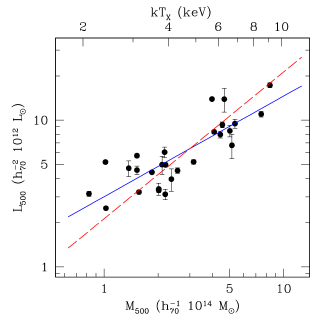
Figure 12: The relation between cluster masses and optical/near-IR luminosities. Left panel: $M_{500}$–$L_{500}$ relation from 2003ApJ…591..749L , using K–band data from the 2MASS survey and masses from X–ray data. The solid line is the best–fit power law, while the dashed line marks the unity slope. Right panel: the same relation, but in the $i$Sloan band. Open and filled points corresponds to mass estimates based on the SDSS spectroscopic data and on the $M$–$T_{X}$ relation, respectively.

Popesso et al. 2005A&A…433..431P analysed SDSS data for a set of clusters which have been identified in the RASS. Their mass estimates come from both X–ray temperature RE02.1 and from the velocity dispersions as estimated from the SDSS spectroscopic data. The results of their analysis for the $i$ band are shown in the right panel of Fig. 12. Again, the optical luminosity correlates quite tightly with the cluster mass, with an intrinsic scatter which is comparable to, or even smaller than that of the correlation between X–ray luminosity and mass.

These results highlight how cluster samples with precisely measured optical luminosities can in principle be usefully employed to constrain cosmological parameters. However, while X-ray luminosity provides at the same time a tracer of cluster mass and a criterion to precisely determine the sample selection function, the latter quantity can be extracted from an optically selected sample only in a rather indirect way.

6 Constraints on cosmological parameters

In this section we will review critically results on cosmological constraints derived from different ways of tracing the cosmological mass function of galaxy clusters.

6.1 The distribution of velocity dispersions

A first determination of the mass function from velocity dispersions, $\sigma_{v}$, of member galaxies has been attempted in 1993ApJ…411L..13B . Girardi et al. 1998ApJ…506…45G used a much larger sample of nearby clusters with measured velocity dispersions to compare the resulting mass function with predictions from cosmological models. The resulting relation between $\sigma_{8}$ and $\Omega_{m}$ was such that $\sigma_{8}\simeq 1$ for a fiducial value of the density parameter $\Omega_{m}=0.3$. More recently, data for nearby clusters, identified in the SDSS, have been used to calibrate a relation between richness and velocity dispersion 2003ApJ…585..182B . They compared the resulting $\sigma_{v}$–distribution to the prediction of cosmological models and found a significantly lower normalization of the power spectrum, $\sigma_{8}\simeq 0.7$ for $\Omega_{m}=0.3$. Such differences from different analyses highlight the presence of systematic uncertainties in the relation between mass and observables (i.e., velocity dispersion and richness).

The application of this method to distant clusters has been applied so far only to the CNOC sample 1997ApJ…479L..19C , which comprises 17 clusters selected from the EMSS out to $z\simeq 0.6$. Still to date, this is the only sample of distant clusters, with calibrated selection function, for which velocity dispersions have been reliably measured. Bahcall et al. 1997ApJ…485L..53B pointed out that the resulting evolution of the mass function is consistent with a low–density Universe. Borgani et al. 1999ApJ…527..561B reanalysed this same sample and emphasised that the uncertainties in the local normalization of the mass function are large enough to make any constraints on $\Omega_{m}$ not significant.

6.2 The temperature function

The X-ray Temperature Function (XTF) is defined as the number density of clusters with given temperature, $n(T)$. As long as a one-to-one relation exist between temperature and mass, the XTF can be related to the mass function, $n(M)$, by the relation

$$n(T)\,=\,n[M(T)]\,{dM\over dT}\,.$$ (45)

In this equation, the ratio $dM/dT$ is provided by the relation between ICM temperature and cluster mass.

Measurements of cluster temperatures for flux-limited samples of nearby clusters were first presented in 1991ApJ…372..410H . These results have been subsequently refined and extended to larger samples with the advent of ROSAT, Beppo–SAX and, especially, ASCA. XTFs have been computed for both nearby (e.g., 1998ApJ…504…27M ; 2001MNRAS.325…77P ; 2003MNRAS.342..163P ; 2002A&A…383..773I ) and distant (e.g., 1998MNRAS.298.1145E ; 1999ApJ…523L.137D ; 2000ApJ…534..565H ; 2004ApJ…609..603H ) clusters, and used to constrain cosmological models. The starting point in the computation of the XTF is inevitably a flux-limited sample for which the searching volume of each cluster can be computed. Then the $L_{X}-T_{X}$ relation and its scatter is used to derive a temperature limit from the sample flux limit.

Once the XTF is measured from observations, eq.(45) is used to infer the mass function and, therefore, to constrain cosmological models. A slightly different but conceptually identical approach, has been followed in RE02.1 , where masses for a flux–limited sample of nearby bright RASS clusters have been computed by applying the assumption of hydrostatic equilibrium, thereby expressing their results directly in terms of mass function, rather than of XTF.

Oukbir and Blanchard 1992A&A…262L..21O first suggested to use the evolution of the XTF as a way to constrain the value of $\Omega_{m}$. Several independent analyses converge now towards a mild evolution of the XTF, which is interpreted as a case for a low–density Universe, with $0.2\raise-2.0pt\hbox{\hbox to0.0pt{\hbox{$\sim$}\hss}\raise 5.0pt\hbox{$<$}\ }\Omega_{m}\raise-2.0pt\hbox{\hbox to0.0pt{\hbox{$\sim$}\hss}\raise 5.0pt\hbox{$<$}\ }0.6$. An example is reported in the right panel of Figure 13 (from 2004ApJ…609..603H ), which shows the comparison between the XTFs of the sample of nearby clusters 1991ApJ…372..410H and a sample of EMSS clusters with ASCA temperatures.

A limitation of the XTFs presented so far is the limited sample size (with only a few $z\raise-2.0pt\hbox{\hbox to0.0pt{\hbox{$\sim$}\hss}\raise 5.0pt\hbox{$>$}\ }0.5$ measurements), as well as the lack of a homogeneous sample selection for local and distant clusters. By combining samples with different selection criteria one runs the risk of altering the inferred evolutionary pattern of the cluster population. This can even give results consistent with a critical–density Universe 1997ApJ…488..566C ; 1999MNRAS.303..535V ; 2000A&A…362..809B .

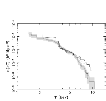
Figure 13: Left panel: a comparison between the XTF for nearby clusters from 2002A&A…383..773I (shaded area), 1998ApJ…504…27M (solid line)and 2000ApJ…534..565H (dotted line). Right panel: the evolution of the XTF from 2004ApJ…609..603H . Open and filled circles are for the local and the distant cluster sample, respectively.

Besides the determination of the matter density parameter, the observational determination of the XTF also allows one to measure the normalization of the power spectrum, $\sigma_{8}$. Assuming a fiducial value of $\Omega_{m}=0.3$, different (sometimes discrepant) determinations of $\sigma_{8}$ have been reported by different authors, ranging from $\sigma_{8}\simeq 0.7$–0.8 (e.g., 1998MNRAS.298.1145E ; RE02.1 ; 2004ApJ…609..603H ) to $\sigma_{8}\simeq 1$ (e.g., 1998ApJ…504…27M ; 2001MNRAS.325…77P ). Ikebe et al. 2002A&A…383..773I compared different observational determinations of the XTF for nearby clusters (see left panel of Fig. 13) and established that they all agree with each other reasonably well. Although quite comfortable, this result highlights that the discrepant results on the normalization of the $\sigma_{8}$–$\Omega_{m}$ relation comes from the cosmological interpretation of the observed XTF, and not from observational uncertainties in its calibration. While the different model mass functions (i.e., whether Press–Schechter, Jenkins et al. or Sheth–Tormen) can in some cases account for part of the difference, more in general the different results are interpreted in terms of the different normalization of the $M$–$T$ relation to be used in eq.(45) or to the way in which the intrinsic scatter and the statistical uncertainties in this relation are included in the analysis. We shall critically discuss these issues in Section 6.5 below.

Substantially improved observational determinations of the XTF, and correspondingly tighter cosmological constraints, are expected to emerge with the accumulations of data on the ICM temperature from the Chandra and XMM–Newton satellites. Thanks to the much improved sensitivity of these X–ray telescopes with respect to ASCA, temperature gradients can be measured for fairly large sets of nearby and medium–distant ($z\raise-2.0pt\hbox{\hbox to0.0pt{\hbox{$\sim$}\hss}\raise 5.0pt\hbox{$<$}\ }0.4$) clusters, thus allowing more precise determinations of cluster masses. At the same time, reliable measurements of global temperatures are now emerging for clusters out to the highest redshifts where they have been secured (e.g., 2004AJ….127..230R ). At the time of writing, several years after the advent of the new generation of X–ray telescopes, no determinations of the XTF from Chandra and XMM–Newton data have been presented, a situation that is expected to change quite soon.

6.3 The luminosity function

Another method to trace the evolution of the cluster number density is based on the X–ray luminosity function (XLF), $\phi(L_{X})$, which is defined as the number density of galaxy clusters having a given X–ray luminosity. Similarly to eq.(45), the XLF can be related to the cosmological mass function of collapsed halos as

$$\phi(L_{X})\,=\,n[M(L_{X})]\,{dM\over dL_{X}}\,,$$ (46)

where $M(L_{X})$ provides the relation between the observable $L_{X}$ and the cluster mass. The above relation needs to be suitably modified in case an intrinsic scatter exists in the relation between mass and temperature (see Section 6.5, here below).

A useful observational quantity, that is related to the XLF, is given by the flux number–counts, $n(S)$, which is defined as the number of clusters per steradian, having measured flux $S$:

$$n(S)\,=\,\left({c\over H_{0}}\right)^{3}\int_{0}^{\infty}dz\,{r^{2}(z)\over E(z)}\,n[M(S,z);z]\,{dM\over dS}$$ (47)

(e.g., 1997ApJ…490..557K ) where $r(z)$ is the radial coordinate appearing in the Friedmann–Robertson–Walker metric:

$$r(z) \!=\! \int_{0}^{z}dz\,E^{-1}(z)~{}~{}~{}~{}~{};~{}~{}~{}~{}~{}\Omega_{\Lambda}=1-\Omega_{m}$$

$$r(z) \!=\! {2\left[\Omega_{m}z+(2-\Omega_{m})\,(1-\sqrt{1+\Omega_{m}z})\right]\over\Omega_{m}^{2}(1+z)}~{}~{}~{};~{}~{}~{}\Omega_{\Lambda}=0\,.$$ (48)

The flux $S$ is related to the luminosity according to

$$S\,=\,{L_{X}\over 4\pi d_{L}^{2}(z)}\,,$$ (49)

where $d_{L}(z)=r(z)(1+z)$ is the luminosity distance at redshift $z$.

This quantity can be measured for a flux–limited samples without having information on cluster redshift and provides useful cosmological information in the absence of any spectroscopic optical follow–up. A comparison between different observational determinations of the flux number counts for both nearby and distant cluster samples (e.g., 2002ARA&A..40..539R ) show indeed a quite good agreement.

Another quantity, which has been used to derive cosmological constraints from flux–limited surveys, is the redshift distribution, $n(z)$, which is defined as the number of clusters found in a survey at a given redshift $z$:

$$n(z)=\left({c\over H_{0}}\right)^{3}\,{r^{2}(z)\over E(z)}\,\int_{S_{lim}}^{\infty}dS\,f_{sky}(S)\,n[M(S,z);z]\,{dM\over dS}\,.$$ (50)

In the above expression $S_{lim}$ is the limiting completeness flux of the survey, while $f_{sky}(S)$ is the effective flux–dependent sky–coverage appropriate for the considered survey. Convolving the mass function with the sky coverage inside the integral in the above equation is essential to properly account for the different effective area covered at different fluxes, an aspect which is apparently overlooked in some analyses (e.g., 2003A&A…412L..37V ).

In general, the advantage of using X-ray luminosity as a tracer of the mass is that $L_{X}$ is measured for a much larger number of clusters in samples with well-defined selection properties. As discussed in Section 4.2, the most recent flux–limited cluster samples contain now a fairly large ($\sim\!100$) number of objects, which are homogeneously identified over a broad redshift baseline, out to $z\simeq 1.3$. This allows nearby and distant clusters to be compared within the same sample, i.e. with a single selection function. However, since the X–ray emissivity depends on the square of the gas density, the relation between $L_{X}$ and $M_{\rm vir}$, which is based on additional physical assumptions, is more uncertain than the $M_{\rm vir}$–$\sigma_{v}$ or the $M_{\rm vir}$–$T$ relations.

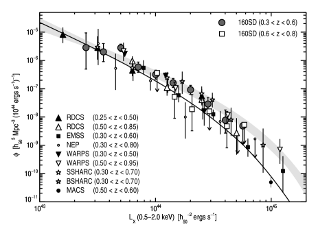
Figure 14: A compilation of XLF within different redshift intervals for independent X–ray flux–limited surveys (from 2004ApJ…607..175M ). The shaded area shows the range of determinations of the local XLF, while the solid curve is the best–fitting evolving XLF from 2004ApJ…607..175M .

A useful parametrization for the relation between temperature and bolometric luminosity can be casted in the form

$$L_{bol}\,=\,L_{6}\,\left({T_{X}\over 6{\rm keV}}\right)^{\alpha}(1+z)^{A}\left({d_{L}(z)\over d_{L,EdS}(z)}\right)^{2}\,10^{44}h^{-2}\,{\rm erg\,s^{-1}}\,,$$ (51)

with $L_{6}$ defining the normalization of the relation and $d_{L}(z)$ the luminosity–distance at redshift $z$ for a given cosmology.

Analyses of the number counts from different X-ray flux–limited cluster surveys showed that the resulting constraints on $\Omega_{m}$ are rather sensitive to the evolution of the mass–luminosity relation 1997ApJ…490..557K ; 1998MNRAS.295..769M ; 1999ApJ…527..561B . On the other hand, other authors 1998A&A…329…21S ; 1999ApJ…518..521R ; 2003A&A…412L..37V analysed different flux–limited surveys and found results consistent with $\Omega_{m}=1$. Quite intriguingly, this conclusion is common to analyses which combine a normalization of the local mass function, using nearby clusters, and to the evolution of the mass function using deep surveys. Clearly, any uncertainty in the calibration of the selection functions when combining different surveys may induce a spurious signal of evolution of the cluster population, possibly misinterpreted as an indication for high $\Omega_{m}$.

In order to overcome this potential problem, Borgani et al. 2001ApJ…561…13B analyzed the RDCS sample to trace the cluster evolution over the entire redshift range, $0.05\raise-2.0pt\hbox{\hbox to0.0pt{\hbox{$\sim$}\hss}\raise 5.0pt\hbox{$<$}\ }z\raise-2.0pt\hbox{\hbox to0.0pt{\hbox{$\sim$}\hss}\raise 5.0pt\hbox{$<$}\ }1.3$, probed by this survey, without resorting to any external normalization from a different survey of nearby clusters 1999ApJ…517…40B . They found $0.1\raise-2.0pt\hbox{\hbox to0.0pt{\hbox{$\sim$}\hss}\raise 5.0pt\hbox{$<$}\ }\Omega_{m}\raise-2.0pt\hbox{\hbox to0.0pt{\hbox{$\sim$}\hss}\raise 5.0pt\hbox{$<$}\ }0.6$ at the $3\sigma$ confidence level, by allowing the $M$–$L_{X}$ relation to change within both the observational and the theoretical uncertainties. In Figure 15 we show the resulting constraints on the $\sigma_{8}$–$\Omega_{m}$ plane (from 2002ARA&A..40..539R ) and how they vary by changing the parameters defining the $M$–$L_{X}$ relation: the slope $\alpha$ and the evolution $A$ of the $L_{X}$–$T$ relation (see Equation 51), the normalization $\beta$ of the $M$–$T$ relation (see Equation 36), and the overall scatter $\Delta_{M-L_{X}}$. Flat geometry is assumed here, i.e. $\Omega_{m}+\Omega_{\Lambda}=1$.

Similar results have been obtained by combining information on clustering properties and the redshift distribution from the the REFLEX cluster survey 2002MNRAS.335..807S , thus providing $\sigma_{8}\simeq 0.7$ and $\Omega_{m}\simeq 0.35$. One should however notice that, since these constraints are derived from nearby clusters, the corresponding estimate of $\Omega_{m}$ comes from the shape of the CDM power spectrum, rather than from the growth rate of perturbations. It is rather reassuring that dynamical and geometrical constraints on $\Omega_{m}$ are in fact consistent with each other.

Constraints on $\Omega_{m}$ from the cluster X–ray luminosity and temperature distribution are thus in line with the completely independent constraints derived from the baryon fraction in clusters, $f_{\rm bar}$ (e.g., 1993Natur.366..429W ; 2003A&A…398..879E ; 2004MNRAS.353..457A ).

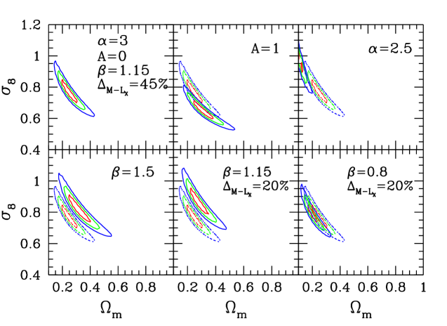
Figure 15: Probability contours in the $\sigma_{8}$–$\Omega_{m}$ plane from the evolution of the X-ray luminosity distribution of RDCS clusters. The shape of the power spectrum is fixed to $\Gamma=0.2$ 2002ARA&A..40..539R . Different panels refer to different ways of changing the relation between cluster virial mass, $M$, and X-ray luminosity, $L_{X}$, within theoretical and observational uncertainties (see also 2001ApJ…561…13B ). The upper left panel shows the analysis corresponding to the choice of a reference parameter set. In each panel, we indicate the parameters which are varied, with the dotted contours always showing the reference analysis.

6.4 The gas mass function

An alternative way of tracing the mass function of galaxy clusters is based on using as its proxy the mass function of the cluster gas content 2003ApJ…590…15V . This method is based on the assumption that galaxy clusters are fair containers of cosmic baryons. Similarly to the method based on the baryon fraction, it relies on the knowledge of the cosmic baryon fraction, either provided by data on the deuterium abundance in high–redshift absorption systems (e.g., 2003ApJS..149….1K ) combined with predictions of primordial nucleosynthesis, or from the spectrum of CMB anisotropies (e.g., 2005astro.ph..7503M ; 2006astro.ph..3449S ). This method has the potential advantage that cluster gas mass is an easier quantity to measure than the total collapsed mass, since it is essentially related to the total cluster emissivity.

If we define $n_{b}(M_{b})$ to be the baryonic mass function and $n(M)$ the total mass function, by definition we have $n_{b}(M_{b})=n(\Omega_{m}M_{b}/\Omega_{b})$. Therefore, once $n_{b}(M_{b})$ and $\Omega_{b}$ are known from observations, the total mass function can be computed as a function of $\Omega_{m}$, thereby treated as a fitting parameter.

While this method has the remarkable advantage of avoiding the uncertainties related to direct estimates of the total collapsed mass, it is affected by possible violations of the assumption of universality of the baryon content of clusters. Indeed, while this assumption should be valid for suitably relaxed and massive clusters, it may be less so when considering all objects belonging to a flux–limited sample, thus including also relatively small clusters and structures with a complex non–relaxed dynamics.

This method was applied 2004ApJ…601..610V to a set of bright clusters selected from the RASS RE02.1 and found $\sigma_{8}=0.72\pm 0.04$ with $\Omega_{m}h=0.13\pm 0.07$. Chandra observations were included in the analysis for a set of clusters extracted from the 160 deg² survey 2003ApJ…590…15V . They found an evolution of the gas mass function, which is consistent with a flat cosmological model with $\Omega_{m}=0.3$.

We emphasize here that the above different methods used to reconstruct the mass function of galaxy clusters consistently prefer relatively low values of $\sigma_{8}$, in the range 0.7–0.8. Quite remarkably, such values have been shown now to be required by the 3–years WMAP data release (2006astro.ph..3449S ).

6.5 Including uncertainties in the analysis

As we have discussed in the previous sections, most of the analyses of the cluster populations converge toward a low–density model, with $\Omega_{m}\sim 0.3$. However, significant differences exist between different determinations of the normalization of the power spectrum, $\sigma_{8}$, which amount to up to $\sim 20$ per cent. These differences are much larger that the statistical uncertainties associated to the finite number of clusters included in the samples, thus indicating that they arise from unaccounted sources of error, which affects the analyses.

For instance, the role of the uncertain normalization of the mass–temperature relation in the determination of $\sigma_{8}$ (at fixed $\Omega_{m}$) from the XTF analysis has been emphasized by different authors (e.g., 2002A&A…383..773I ; 2003MNRAS.342..163P ; 2002MNRAS.337..769S ). Increasing the normalization of the $M$–$T$ relation implies that a larger mass corresponds to a fixed temperature value. As a consequence, an observed XTF translates into a larger mass function, therefore implying a larger $\sigma_{8}$ (at fixed $\Omega_{m}$). Since results from hydrodynamical simulations generally imply a larger $M$–$T$ normalization, a larger $\sigma_{8}$ is expected when using in the analysis the simulation predictions. The left panel of Figure 16 (from 2002A&A…383..773I ) shows how the best fitting values of $\sigma_{8}$ and $\Omega_{m}$ from the local XTF change as one uses different mass–temperature relations, taken from both observations and simulations. The right panel of Fig.16 (from 2003MNRAS.342..163P ) show the dependence of $\sigma_{8}$ on the normalization of the mass–temperature relation. Note that this normalization is allowed here to vary over the range encompassed by observational and simulation results. The range of variation of $\sigma_{8}$ induced by the uncertainty in the $M$–$T$ relation is at least comparable to the purely statistical uncertainty, as indicated by the errorbars.

One may wonder why not relying only on the observational determination of the $M$–$T$ relation, instead of considering also simulation results. As we shall discuss in Section 7, observational results can not necessarily provide the most reliable determination of the $M$–$T$ scaling.

Figure 16: Left panel: the dependence of the best–fitting values of $\Omega_{m}$ and $\sigma_{8}$, from the XTF of 2002A&A…383..773I , upon different determinations of the mass–temperature relation, from both observational data and from hydrodynamical simulations of galaxy clusters. Right panel: the dependence of $\sigma_{8}$ on the normalization of the mass–temperature relation, in the XTF analysis by 2003MNRAS.342..163P .

The effect of changing the normalization of the $M$–$T$ relation on the analysis of flux–limited samples through the XLF evolution is shown in the lower left panel of Fig.15. If this normalization is reduced by $\sim\!30\%$, the resulting $\sigma_{8}$ decreases by $\sim\!20\%$.

It is clear that, any uncertainty, both statistical and systematic, in the fitting parameters describing the scaling relations between mass and observable, must be included in the analysis by marginalizing over the probability distribution function of these parameters. Let ${\bf\Omega}$ be the set of cosmological parameters that we want to constrain, and ${\bf W}$ the set of parameters which define a scaling relation between mass $M$ and an observable $X$ (i.e., $\sigma_{v}$, $L_{X}$ or $T$). Let us also call $P({\bf W})$ the prior distribution for the uncertainties in the $M$–$X$ relation. If $\chi^{2}({\bf\Omega},{\bf W})$ gives the goodness of fit provided by the choice ${\bf\Omega}$ of the cosmological parameters, for a given $M$–$X$ relation, then the goodness of fit after marginalizing over the uncertainties in $M$–$X$ reads

$$\chi^{2}({\bf\Omega})\,=\,{\int\chi^{2}({\bf\Omega},{\bf W})\,P({\bf W})\,d{\bf W}\over\int P({\bf W})\,d{\bf W}}\,.$$ (52)

Of course, the marginalization generally induces an increase of the uncertainties in the cosmological parameters. Furthermore, one needs to have a reliable modeling of both size and distribution of the errors (i.e. whether they have a uniform, a Gaussian, or a more peculiar distribution).

Besides the errors in the parameters defining the scaling relations, a different source of uncertainty is provided by the intrinsic scatter in these relations. Intrinsic scatter has the effect of widening the range of possible masses which correspond to a given value of the observable quantity. This effect can be included in the analysis by convolving the theoretical mass function with the distribution of the scatter itself (e.g., 2001ApJ…561…13B ; 2005PhRvD..72d3006L ). Let $\Psi$ be an observable quantity and $\phi(\Psi)$ its distribution (i.e., XLF or XTF), to be compared with observations. Also, let $P(M_{\Psi}|M;z)$ be the probability of assigning a mass $M_{\Psi}$ to a cluster of true mass $M$, at redshift $z$, from the observable $\Psi$, for a given $M$–$\Psi$ relation. Therefore, the model prediction for the distribution $\phi(\Psi)$, to be compared with its observational determination, is given by the convolution of the cosmological mass function with the distribution of the intrinsic scatter:

$$\phi(\Psi)d\Psi\,=\,\int dM_{\Psi}n(M_{\Psi},z)\,P(M_{\Psi}|M;z)\,{dM\over d\Psi}\,d\Psi$$ (53)

where $n(M,z)$ is the cosmological mass function at redshift $z$. If one makes the standard assumption of Gaussian scatter in the log–log plane, then

$$P(M_{\Psi}|M)\,=\,\left(2\pi\sigma_{\ln M}^{2}\right)^{-1/2}\exp\left[-x^{2}(M_{\Psi})\right]\,,$$ (54)

where $x(M_{\Psi})=(\ln M_{\Psi}-\ln M)/(\sqrt{2}\sigma_{\ln M})$ and $\sigma_{\ln M}$ is the r.m.s. intrinsic scatter. The effect of this convolution is that of increasing $\phi(\Psi)$, for a fixed $n(M)$, as the scatter increases. Therefore, assuming a progressively larger scatter in the $M$–$\Psi$ relation implies a progressively lower $\sigma_{8}$ (at fixed $\Omega_{m}$). An illustrative example of the effect of intrinsic scatter on the determination of $\sigma_{8}$ is reported in Figure 17. In the left panel we show the REFLEX XLF 2002ApJ…566…93B along with the prediction of the best fitting cosmological model for a given choice of the $M$–$L_{X}$ relation, after assuming vanishing intrinsic scatter in this relation. In the left panel, we show the same comparison, but assuming an Gaussian–distributed intrinsic scatter of 40 per cent in the $M$–$L_{X}$ scaling. As expected, adding the scatter has the effect of increasing the predicted luminosity function, so that $\sigma_{8}$ has to be lowered from 0.8 to 0.65 to recover the agreement with observations.

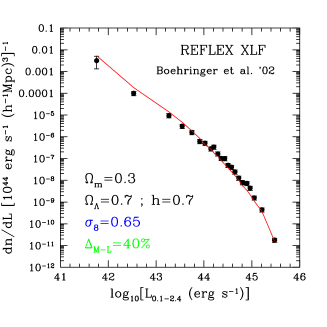
Figure 17: The dependence of $\sigma_{8}$ on the intrinsic scatter assumed in the relation between X–ray luminosity and mass. The two panels show the comparison between model predictions and the observed XLF from the REFLEX sample 2002ApJ…566…93B . The left panel assumes vanishing scatter while the right panel assumes a 40 per cent intrinsic scatter. The best fitting values of $\sigma_{8}$ are reported in both cases.

This example highlights that a good calibration of the intrinsic scatter in the scaling relations can be as important as determining the best–fitting amplitude and slope of these relations.

7 The future

A new era for cosmology with galaxy clusters is now starting. High sensitivity surveys for blind SZ identification over fairly large contiguous area, $\sim 100$ deg², have have already started or are planned in the coming years (see the lectures by M. Birkinshaw in this volume). Also, the Planck satellite will survey the whole sky, although at a much lower sensitivity, and provide a large set of clusters identified through the SZ effect. These surveys promise to identify several thousands clusters, with a fair number of objects expected to be found at $z>1$. In the optical/near-IR bands, imaging with dedicated telescopes with large field of view will also allow to secure a large number of distant clusters. At the same time, X–ray observations over contiguous area (e.g., 2005MNRAS.363..675W and “serendipitous” searches from XMM–Newton (e.g., 2005ApJ…623L..85M ) and Chandra (e.g., 2002A&A…396..397B ) archives will ultimately cover several hundreds deg² down to flux limits fainter than those reached by the deepest ROSAT pointings. Preliminary results suggest that identification of $z>1$ clusters may eventually become routine 2005ApJ…623L..85M . Ultimately, they will lead to the identification of several thousands clusters.

Optimized optics for wide–field X–ray imaging have been originally described in a far-reaching paper by Burrows et al. 1992ApJ…392..760B and proposed for the first time to be implemented in a dedicated satellite mission in the mid 90’s. There is no doubt that this would be the right time to plan a dedicated wide–field X–ray telescope, which should survey the sky over an area of several thousands deg², with a relatively good, XMM–like or better, point spread function and a low background. This instrument would be invaluable for studies of galaxy clusters, thanks to its ability of both identifying extended sources with low surface brightness. Several missions with a similar profile have been proposed, although none has been approved so far. Still, the community working on galaxy clusters is regularly proposing this idea of satellite to different Space Agencies (e.g., 2005astro.ph..7013H ).

The samples of galaxy clusters obtainable from large–area SZ and X–ray surveys contain in principle so much information to allow one to constrain not only $\Omega_{m}$ and $\sigma_{8}$, but also the Dark Energy (DE) content of the Universe (see, e.g., 2003RSPTA.361.2497S ; 2005LNP…653..141S for introductory reviews on Dark Energy). The equation of state of DE is written in the form $p=w\rho$, where $p$ and $\rho$ are the pressure and density terms, respectively. The parameter $w$ must take values in the range $-1/3>w\geq-1$ for the DE to provide an accelerated cosmic expansion. Constraining the value of $w$ and its redshift evolution is currently considered one of the most ambitious targets of modern cosmology. Ones hope is to unveil the nature of the energy term which dominates the overall dynamics of the Universe at the present time.

As we have mentioned, the limited statistics prevents current cluster surveys to place significant constraints on $\Omega_{\Lambda}$. Although this limitation will be overcome with future cluster surveys, the question remains as to whether the systematic effects, discussed in Section 6.5, can be sufficiently understood. Different lines of attack have been proposed in the literature, which should not considered as alternative to each other.

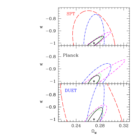
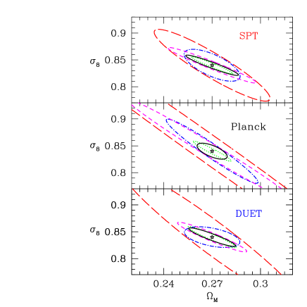
Figure 18: Constraints on cosmological parameters from the SZ SPT survey, from the SZ Planck survey and from a wide–area deep X–ray survey (from top to bottom panels; from 2004ApJ…613…41M ). Dotted lines: no uncertainty in the relation between cluster mass and observables, using only the $dn/dz$ information; long–dashed line: using self–calibration on the $dn/dz$; dot–dashed line: as before, but also including the information on the cluster power spectrum; short–dashed line: using $dn/dz$ and a calibration of the mass–observable relation for 100 clusters; solid line: all the information combined together.

Majumdar and Mohr 2004ApJ…613…41M have proposed the approach based on the so–called self–calibration (see also 2003ApJ…585..603M ; 2004PhRvD..70d3504L ; 2005PhRvD..72d3006L ). The idea underlying this approach is that of parametrizing in a sensible way the scaling relations between cluster observables and mass, including the corresponding intrinsic scatter and its distribution. In this way, the parameters describing these relations can be considered as fitting parameter to be added to the cosmological parameters. As long as the cluster samples are large enough, one should be able to fit at the same time both cosmological parameters and those parameters related to the physical properties of clusters. Figure 18 (from 2004ApJ…613…41M ) shows the constraints that one can place on the $w$–$\Omega_{m}$ (left panel) and on the $\sigma_{8}$–$\Omega_{m}$ planes, after marginalizing over the other fitting parameters, from different SZ and X–ray surveys. In each panel different contours indicate the constraints that one can place by progressively adding information in the analysis. The main message here is that combining information on the evolution of the cluster population and on its clustering can place precision constraints on cosmological parameters. These constraints can be further tightened if follow up observations are available to precisely measure masses for 100 clusters.

These forecasts nicely illustrates the potentiality of the self–calibration approach for precision cosmology with future surveys of galaxy clusters. Clearly, the robustness of these predictions is inextricably linked to the possibility of accurately modeling the relations between mass and observables.

A line of attack to this problem is based on using detailed hydrodynamical simulations of galaxy clusters. The great advantages of using simulations is that both cluster mass and observable quantities can be exactly computed. Furthermore, the effect of observational set–ups (e.g., response functions of detectors, etc.) can be included in the analysis and their effect on the scaling relations quantified. This approach has been applied by different groups in the case of X–ray observations 2004MNRAS.351..505G to understand the relation between the ICM temperature, as measured from the fitting of the observed spectrum, and the “true” mass–weighted temperature (e.g., 2001ApJ…546..100M ; 2004MNRAS.354…10M ; 2005astro.ph..4098V ). Furthermore, simulations can also be used to verify in detail the validity of assumptions on which the mass estimators, applied to observations, are based. The typical example is represented by the assumption of hydrostatic equilibrium, discussed in Sect.5.1, for which violations in simulations at the 10–20 per cent level have been found (e.g., 1996MNRAS.283..431B ; 2004MNRAS.351..237R ; 2004MNRAS.348.1078B ; 2004MNRAS.355.1091K ).

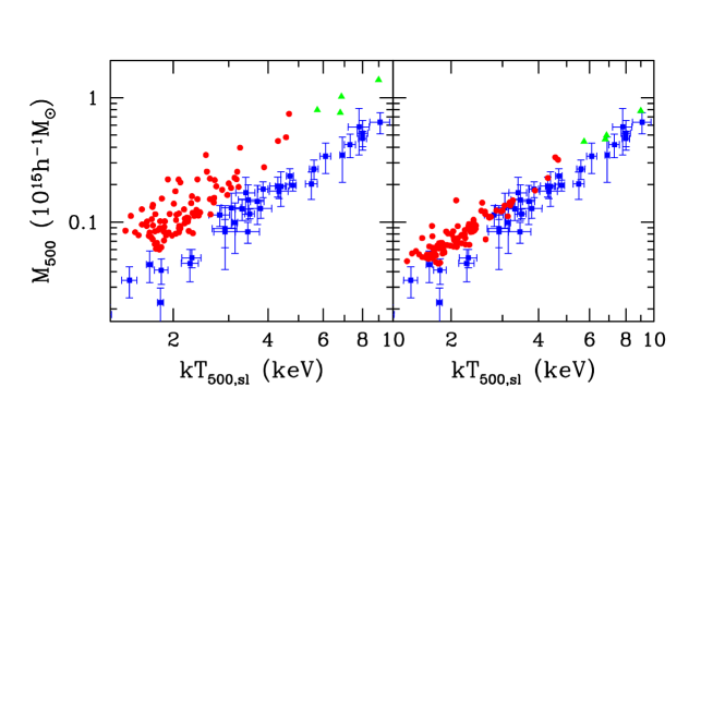
Figure 19: The mass–temperature relation at $\bar{\rho}/\rho_{\rm cr}=500$, in simulations (filled circles and triangles) and for the observational data (squares with errorbars, 2001A&A…368..749F ). The left panel is for the true masses of simulated clusters; the right panel is for masses of simulated clusters estimated by adopting the same procedure applied by Finoguenov et al. to observational data (from 2005ApJ…618L…1R ).

An example of calibration of observational biases in the mass–temperature relation, using hydrodynamical simulations, is shown in Figure 19 (from 2005ApJ…618L…1R ), which provides a comparison between the observed and the simulated $M$–$T$ relation. Simulations here include radiative cooling, star formation and the effect of galactic winds powered by supernovae, and, as such, provide a realistic description of the relevant physical processes. The observational results, which are taken from 2001A&A…368..749F , corresponds to mass estimates based on the hydrostatic equilibrium for a polytropic $\beta$–model of the gas distribution [eq.(33)]. In both panels, the temperature has been computed by using a proxy to the actual spectroscopic temperature, the so–called spectroscopic–like temperature 2004MNRAS.354…10M . The left panel shows the results when exact masses of simulated clusters are used for the comparison. Based on this result only, the conclusion would be that simulations do indeed produce too high a $M$–$T$ relation, even in the presence of a realistic description of gas physics. In the left panel, masses of simulated clusters are computed instead by using the same procedure as for observed clusters, i.e. by applying eq.(34) for the hydrostatic equilibrium of a polytropic $\beta$–model. Quite remarkably, the effect of applying the observational mass estimator has two effects. First, the overall normalization of the $M$–$T$ relation is decreased by the amount required to attain a reasonable agreement with observations. Second, the scatter in the simulated $M$–$T$ relation is substantially suppressed. This is the consequence of the fact that eq.(34) provides a one-to-one correspondence between mass and temperature, while only the cluster-by-cluster variations of $\beta$ and $\gamma$ account for the intrinsic diversity of the cluster thermal structure.

This example illustrates how simulations can be usefully employed as guidelines to study possible biases on observational mass estimates. However, it is worth reminding that the reliability of simulation results depends on our capability to correctly provide a numerical description of all the relevant physical process. In this sense, understanding in detail the (astro)physics of clusters is mandatory in order to calibrate them as tools in the era of precision cosmology.

As a concluding remark, we emphasize once more that a number of independent analysesof the cluster mass function, which have been realized so far, favor a relatively low normalization of the power spectrum, with $\sigma_{8}\simeq 0.7$–0.8 for $\Omega_{m}\simeq 0.3$, thus in agreement with the most recent WMAP results (2006astro.ph..3449S ). This agreement must be considered as a success for cluster cosmology and a strong encourgement for future applications to large cluster surveys of the next generation.

Acknowledgments. I would like to thank the organizers of the GH2005 School, David Hughes, Omar Lopez–Cruz and Manolis Plionis for having provided an enjoyable and stimulating environment. I also warmly thank Manolis Plionis and Piero Rosati for a careful reading of the manuscript and useful suggestions to improve it.

References

- (1) Abell G. O., 1958, ApJS, 3, 211
- (2) Abell G. O., Corwin H. G., Olowin R. P., 1989, ApJS, 70, 1
- (3) Allen S. W., Fabian A. C., 1998, MNRAS, 297, L57
- (4) Allen S. W., Schmidt R. W., Ebeling H., Fabian A. C., van Speybroeck L., 2004, MNRAS, 353, 457
- (5) Allen S. W., Schmidt R. W., Fabian A. C., 2001, MNRAS, 328, L37
- (6) Allen S. W., Schmidt R. W., Fabian A. C., 2002, MNRAS, 334, L11
- (7) Arnaud M., Evrard A. E., 1999, MNRAS, 305, 631
- (8) Arnaud M., Pointecouteau E., Pratt G. W., 2005, A&A, 441, 893
- (9) Bahcall N. A., Cen R., Dav é R., Ostriker J. P., Yu Q., 2000, ApJ, 541, 1
- (10) Bahcall N. A., Dong F., Bode P., Kim R., Annis J., McKay T. A., Hansen S., Schroeder J., Gunn J., Ostriker J. P., Postman M., Nichol R. C., Miller C., Goto T., Brinkmann J., Knapp G. R., Lamb D. O., Schneider D. P., Vogeley M. S., York D. G., 2003, ApJ, 585, 182
- (11) Bahcall N. A., Fan X., Cen R., 1997, ApJ, 485, L53+
- (12) Bartelmann M., Steinmetz M., 1996, MNRAS, 283, 431
- (13) Basilakos, S., Plionis, M., Georgakakis, A., Georgantopoulos, I., Gaga, T., Kolokotronis, V., Stewart, G., 2004, MNRAS, 351, 989
- (14) Binney J., Tremaine S., 1987, Galactic dynamics . Princeton, NJ, Princeton University Press, 1987, 747 p.
- (15) Birkinshaw M., 1999, Phys. Rep., 310, 97
- (16) Biviano A., Girardi M., 2003, ApJ, 585, 205
- (17) Biviano A., Girardi M., Giuricin G., Mardirossian F., Mezzetti M., 1993, ApJ, 411, L13
- (18) Biviano A., Murante G., Borgani S., Diaferio A., Dolag K., Girardi M., 2006, ArXiv Astrophysics e-prints
- (19) Blanchard A., Sadat R., Bartlett J. G., Le Dour M., 2000, A&A, 362, 809
- (20) B ö hringer H., Collins C. A., Guzzo L., Schuecker P., Voges W., Neumann D. M., Schindler S., Chincarini G., De Grandi S., Cruddace R. G., Edge A. C., Reiprich T. H., Shaver P., 2002, ApJ, 566, 93
- (21) B ö hringer H., Schuecker P., Guzzo L., Collins C. A., Voges W., Cruddace R. G., Ortiz-Gil A., Chincarini G., De Grandi S., Edge A. C., MacGillivray H. T., Neumann D. M., Schindler S., Shaver P., 2004, A&A, 425, 367
- (22) B ö hringer H., Voges W., Huchra J. P., McLean B., Giacconi R., Rosati P., Burg R., Mader J., Schuecker P., Simi ç D., Komossa S., Reiprich T. H., Retzlaff J., Tr ü mper J., 2000, ApJS, 129, 435
- (23) Bond J. R., Cole S., Efstathiou G., Kaiser N., 1991, ApJ, 379, 440
- (24) Borgani S., Girardi M., Carlberg R. G., Yee H. K. C., Ellingson E., 1999, ApJ, 527, 561
- (25) Borgani S., Governato F., Wadsley J., Menci N., Tozzi P., Quinn T., Stadel J., Lake G., 2002, MNRAS, 336, 409
- (26) Borgani S., Guzzo L., 2001, Nature, 409, 39
- (27) Borgani S., Murante G., Springel V., Diaferio A., Dolag K., Moscardini L., Tormen G., Tornatore L., Tozzi P., 2004, MNRAS, 348, 1078
- (28) Borgani S., Rosati P., Tozzi P., Norman C., 1999, ApJ, 517, 40
- (29) Borgani S., Rosati P., Tozzi P., Stanford S. A., Eisenhardt P. R., Lidman C., Holden B., Della Ceca R., Norman C., Squires G., 2001, ApJ, 561, 13
- (30) Boschin W., 2002, A&A, 396, 397
- (31) Bryan G. L., Norman M. L., 1998, ApJ, 495, 80
- (32) Burke D. J., Collins C. A., Sharples R. M., Romer A. K., Holden B. P., Nichol R. C., 1997, ApJ, 488, L83+
- (33) Burrows C. J., Burg R., Giacconi R., 1992, ApJ, 392, 760
- (34) Carlberg R. G., Morris S. L., Yee H. K. C., Ellingson E., 1997, ApJ, 479, L19+
- (35) Carlberg R. G., Yee H. K. C., Ellingson E., Abraham R., Gravel P., Morris S., Pritchet C. J., 1996, ApJ, 462, 32
- (36) Carlberg R. G., Yee H. K. C., Ellingson E., Morris S. L., Abraham R., Gravel P., Pritchet C. J., Smecker-Hane T., Hartwick F. D. A., Hesser J. E., Hutchings J. B., Oke J. B., 1997, ApJ, 476, L7+
- (37) Carlstrom J. E., Holder G. P., Reese E. D., 2002, ARAA, 40, 643
- (38) Castander F. J., Bower R. G., Ellis R. S., Aragon-Salamanca A., Mason K. O., Hasinger G., McMahon R. G., Carrera F. J., Mittaz J. P. D., Perez-Fournon I., Lehto H. J., 1995, Nature, 377, 39
- (39) Cavaliere A., Fusco-Femiano R., 1976, A&A, 49, 137
- (40) Cavaliere A., Gursky H., Tucker W., 1971, Nature, 231, 437
- (41) Colafrancesco S., Mazzotta P., Vittorio N., 1997, ApJ, 488, 566
- (42) Coles P., Lucchin F., 2002, Cosmology: The Origin and Evolution of Cosmic Structure, Second Edition . Cosmology: The Origin and Evolution of Cosmic Structure, Second Edition, by Peter Coles, Francesco Lucchin, pp. 512. ISBN 0-471-48909-3. Wiley-VCH , July 2002.
- (43) Couch W. J., Ellis R. S., MacLaren I., Malin D. F., 1991, MNRAS, 249, 606
- (44) Dalcanton J. J., 1996, ApJ, 466, 92
- (45) Dalton G. B., Maddox S. J., Sutherland W. J., Efstathiou G., 1997, MNRAS, 289, 263
- (46) Davis M., Peebles P. J. E., 1983, ApJ, 267, 465
- (47) Diaferio A., Borgani S., Moscardini L., Murante G., Dolag K., Springel V., Tormen G., Tornatore L., Tozzi P., 2005, MNRAS, 356, 1477
- (48) Donahue, Megan, Scharf, Caleb A., Mack, Jennifer, Lee, Y. Paul, Postman, Marc, Rosati, Piero, Dickinson, Mark, Voit, G. Mark, Stocke, John T., 2002, ApJ, 569, 689
- (49) Donahue M., Mack J., Scharf C., Lee P., Postman M., Rosati P., Dickinson M., Voit G. M., Stocke J. T., 2001, ApJ, 552, L93
- (50) Donahue M., Voit G. M., 1999, ApJ, 523, L137
- (51) Ebeling H., Edge A. C., Allen S. W., Crawford C. S., Fabian A. C., Huchra J. P., 2000, MNRAS, 318, 333
- (52) Ebeling H., Edge A. C., Henry J. P., 2001, ApJ, 553, 668
- (53) Eisenstein D. J., Hu W., 1999, ApJ, 511, 5
- (54) Eke V. R., Cole S., Frenk C. S., 1996, MNRAS, 282, 263
- (55) Eke V. R., Cole S., Frenk C. S., Patrick Henry J., 1998, MNRAS, 298, 1145
- (56) Ettori S., De Grandi S., Molendi S., 2002, A&A, 391, 841
- (57) Ettori S., Tozzi P., Borgani S., Rosati P., 2004, A&A, 417, 13
- (58) Ettori S., Tozzi P., Rosati P., 2003, A&A, 398, 879
- (59) Evrard A. E., MacFarland T. J., Couchman H. M. P., Colberg J. M., Yoshida N., White S. D. M., Jenkins A., Frenk C. S., Pearce F. R., Peacock J. A., Thomas P. A., 2002, ApJ, 573, 7
- (60) Fabian A. C., 1991, MNRAS, 253, 29P
- (61) Felten J. E., Gould R. J., Stein W. A., Woolf N. J., 1966, ApJ, 146, 955
- (62) Finoguenov A., Reiprich T. H., B ö hringer H., 2001, A&A, 368, 749
- (63) Frenk C. S., Evrard A. E., White S. D. M., Summers F. J., 1996, ApJ, 472, 460
- (64) Gardini A., Rasia E., Mazzotta P., Tormen G., De Grandi S., Moscardini L., 2004, MNRAS, 351, 505
- (65) Giacconi R., Branduardi G., Briel U., et al. 1979, ApJ, 230, 540
- (66) Giacconi R., Murray S., Gursky H., Kellogg E., Schreier E., Tananbaum H., 1972, ApJ, 178, 281
- (67) Gioia I. M., Henry J. P., Maccacaro T., Morris S. L., Stocke J. T., Wolter A., 1990, ApJ, 356, L35
- (68) Girardi M., Biviano A., Giuricin G., Mardirossian F., Mezzetti M., 1993, ApJ, 404, 38
- (69) Girardi M., Borgani S., Giuricin G., Mardirossian F., Mezzetti M., 1998, ApJ, 506, 45
- (70) Girardi M., Borgani S., Giuricin G., Mardirossian F., Mezzetti M., 2000, ApJ, 530, 62
- (71) Girardi M., Giuricin G., Mardirossian F., Mezzetti M., Boschin W., 1998, ApJ, 505, 74
- (72) Girardi M., Manzato P., Mezzetti M., Giuricin G., Limboz F., 2002, ApJ, 569, 720
- (73) Girardi M., Mezzetti M., 2001, ApJ, 548, 79
- (74) Gladders M. D., Yee H. K. C., 2005, ApJS, 157, 1
- (75) Gonzalez A. H., Zaritsky D., Dalcanton J. J., Nelson A., 2001, ApJS, 137, 117
- (76) Governato F., Babul A., Quinn T., Tozzi P., Baugh C. M., Katz N., Lake G., 1999, MNRAS, 307, 949
- (77) Gross M. A. K., Somerville R. S., Primack J. R., Holtzman J., Klypin A., 1998, MNRAS, 301, 81
- (78) Gunn J. E., Hoessel J. G., Oke J. B., 1986, ApJ, 306, 30
- (79) Haiman Z., Allen S., Bahcall N., et al. 2005, ArXiv Astrophysics e-prints
- (80) Haiman Z., Mohr J. J., Holder G. P., 2001, ApJ, 553, 545
- (81) Henry J. P., 2000, ApJ, 534, 565
- (82) Henry J. P., 2004, ApJ, 609, 603
- (83) Henry J. P., Arnaud K. A., 1991, ApJ, 372, 410
- (84) Henry J. P., Gioia I. M., Maccacaro T., Morris S. L., Stocke J. T., Wolter A., 1992, ApJ, 386, 408
- (85) Henry J. P., Gioia I. M., Mullis C. R., Voges W., Briel U. G., B ö hringer H., Huchra J. P., 2001, ApJ, 553, L109
- (86) Holden B. P., Stanford S. A., Squires G. K., Rosati P., Tozzi P., Eisenhardt P., Spinrad H., 2002, AJ, 124, 33
- (87) Hu W., Kravtsov A. V., 2003, ApJ, 584, 702
- (88) Ikebe Y., Reiprich T. H., B ö hringer H., Tanaka Y., Kitayama T., 2002, A&A, 383, 773
- (89) Jenkins A., Frenk C., White S., Colberg J., Cole S., Evrard A., Couchman H., Yoshida N., 2001, MNRAS, 321, 372
- (90) Kaiser N., 1986, MNRAS, 222, 323
- (91) Kay S. T., Thomas P. A., Jenkins A., Pearce F. R., 2004, MNRAS, 355, 1091
- (92) Kirkman D., Tytler D., Suzuki N., O’Meara J. M., Lubin D., 2003, ApJS, 149, 1
- (93) Kitayama T., Suto Y., 1996, ApJ, 469, 480
- (94) Kitayama T., Suto Y., 1997, ApJ, 490, 557
- (95) Kotov O., Vikhlinin A., 2005, ApJ, 633, 781
- (96) Lewis A. D., Ellingson E., Morris S. L., Carlberg R. G., 1999, ApJ, 517, 587
- (97) Lima M., Hu W., 2004, Phys. Rev. D, 70, 043504
- (98) Lima M., Hu W., 2005, Phys. Rev. D, 72, 043006
- (99) Limber D. N., Mathews W. G., 1960, ApJ, 132, 286
- (100) Lin Y.-T., Mohr J. J., Stanford S. A., 2003, ApJ, 591, 749
- (101) Lumb D. H., Bartlett J. G., Romer A. K., Blanchard A., Burke D. J., Collins C. A., Nichol R. C., Giard M., Marty P. B., Nevalainen J., Sadat R., Vauclair S. C., 2004, A&A, 420, 853
- (102) Lumsden S. L., Nichol R. C., Collins C. A., Guzzo L., 1992, MNRAS, 258, 1
- (103) MacTavish C., Ade P. A. R., Bock J. J., et al. 2005, ArXiv Astrophysics e-prints
- (104) Majumdar S., Mohr J. J., 2003, ApJ, 585, 603
- (105) Majumdar S., Mohr J. J., 2004, ApJ, 613, 41
- (106) Markevitch M., 1998, ApJ, 504, 27
- (107) Mathiesen B., Evrard A. E., 1998, MNRAS, 295, 769
- (108) Mathiesen B. F., Evrard A. E., 2001, ApJ, 546, 100
- (109) Maughan B. J., Jones L. R., Ebeling H., Scharf C., 2006, MNRAS, 365, 509
- (110) Mazzotta P., Rasia E., Moscardini L., Tormen G., 2004, MNRAS, 354, 10
- (111) Miller C. J., Nichol R. C., Reichart D., et al. 2005, AJ, 130, 968
- (112) Monaco P., 1998, Fundamentals of Cosmic Physics, 19, 157
- (113) Moretti A., Guzzo L., Campana S., Lazzati D., Panzera M. R., Tagliaferri G., Arena S., Braglia F., Dell’Antonio I., Longhetti M., 2004, A&A, 428, 21
- (114) Moscardini L., Matarrese S., Mo H. J., 2001, MNRAS, 327, 422
- (115) Motl P. M., Hallman E. J., Burns J. O., Norman M. L., 2005, ApJ, 623, L63
- (116) Mulchaey J. S., Zabludoff A. I., 1998, ApJ, 496, 73
- (117) Mullis C. R., McNamara B. R., Quintana H., Vikhlinin A., Henry J. P., Gioia I. M., Hornstrup A., Forman W., Jones C., 2003, ApJ, 594, 154
- (118) Mullis C. R., Rosati P., Lamer G., B ö hringer H., Schwope A., Schuecker P., Fassbender R., 2005, ApJ, 623, L85
- (119) Mullis C. R., Vikhlinin A., Henry J. P., Forman W., Gioia I. M., Hornstrup A., Jones C., McNamara B. R., Quintana H., 2004, ApJ, 607, 175
- (120) Nevalainen J., Markevitch M., Forman W., 2000, ApJ, 532, 694
- (121) Osmond J. P. F., Ponman T. J., 2004, MNRAS, 350, 1511
- (122) Oukbir J., Blanchard A., 1992, A&A, 262, L21
- (123) Peacock J. A., 1999, Cosmological Physics . Cosmological Physics, by John A. Peacock, pp. 704. ISBN 052141072X. Cambridge, UK: Cambridge University Press, January 1999.
- (124) Peebles P. J. E., 1993, Principles of physical cosmology . Princeton Series in Physics, Princeton, NJ: Princeton University Press, —c1993
- (125) Perlman E. S., Horner D. J., Jones L. R., Scharf C. A., Ebeling H., Wegner G., Malkan M., 2002, ApJS, 140, 265
- (126) Piccinotti G., Mushotzky R. F., Boldt E. A., Holt S. S., Marshall F. E., Serlemitsos P. J., Shafer R. A., 1982, ApJ, 253, 485
- (127) Pierpaoli E., Borgani S., Scott D., White M., 2003, MNRAS, 342, 163
- (128) Pierpaoli E., Scott D., White M., 2001, MNRAS, 325, 77
- (129) Plionis, M., Basilakos, S., Georgantopoulos, I., Georgakakis, A., 2005, ApJ, 622, L17
- (130) Popesso P., Biviano A., B ö hringer H., Romaniello M., Voges W., 2005, A&A, 433, 431
- (131) Postman M., Lubin L. M., Gunn J. E., Oke J. B., Hoessel J. G., Schneider D. P., Christensen J. A., 1996, AJ, 111, 615
- (132) Press W., Schechter P., 1974, ApJ, 187, 425
- (133) Rasia E., Mazzotta P., Borgani S., Moscardini L., Dolag K., Tormen G., Diaferio A., Murante G., 2005, ApJ, 618, L1
- (134) Rasia E., Tormen G., Moscardini L., 2004, MNRAS, 351, 237
- (135) Reichart D. E., Nichol R. C., Castander F. J., Burke D. J., Romer A. K., Holden B. P., Collins C. A., Ulmer M. P., 1999, ApJ, 518, 521
- (136) Reiprich T., B ö hringer H., 2002, ApJ, 567, 716
- (137) Rines K., Geller M. J., Kurtz M. J., Diaferio A., 2003, AJ, 126, 2152
- (138) Rosati P., Borgani S., Norman C., 2002, ARAA, 40, 539
- (139) Rosati P., della Ceca R., Norman C., Giacconi R., 1998, ApJ, 492, L21+
- (140) Rosati P., Tozzi P., Ettori S., Mainieri V., Demarco R., Stanford S. A., Lidman C., Nonino M., Borgani S., Della Ceca R., Eisenhardt P., Holden B. P., Norman C., 2004, AJ, 127, 230
- (141) Sadat R., Blanchard A., Oukbir J., 1998, A&A, 329, 21
- (142) Sahni V., 2005, LNP Vol. 653: The Physics of the Early Universe, 653, 141
- (143) Schuecker P., B ö hringer H., Guzzo L., Collins C. A., Neumann D. M., Schindler S., Voges W., De Grandi S., Chincarini G., Cruddace R., M ü ller V., Reiprich T. H., Retzlaff J., Shaver P., 2001, A&A, 368, 86
- (144) Schuecker P., Guzzo L., Collins C. A., B ö hringer H., 2002, MNRAS, 335, 807
- (145) Seljak U., 2002, MNRAS, 337, 769
- (146) Sheth R., Tormen G., 1999, MNRAS, 308, 119
- (147) Sheth R. K., Tormen G., 2002, MNRAS, 329, 61
- (148) Smith S., 1936, ApJ, 83, 23
- (149) Spergel D. N., Bean R., Doré O., Nolta M. R., Bennett, C. L., Hinshaw G., Jarosik N., Komatsu E., Page L., Peiris H. V., Verde L., Barnes C., Halpern M., Hill R. S., Kogut A., Limon M., Meyer S. S., Odegard N., Tucker G. S., Weiland J. L., Wollack E., Wright E. L., 2006, ArXiv Astrophysics e-prints
- (150) Springel V., White S. D. M., Jenkins A., Frenk C. S., Yoshida N., Gao L., Navarro J., Thacker R., Croton D., Helly J., Peacock J. A., Cole S., Thomas P., Couchman H., Evrard A., Colberg J., Pearce F., 2005, Nature, 435, 629
- (151) Stanford S. A., Holden B., Rosati P., Eisenhardt P. R., Stern D., Squires G., Spinrad H., 2002, AJ, 123, 619
- (152) Stanford S. A., et al., 2005, ApJ, 634, L129
- (153) Steinhardt P. J., 2003, Royal Society of London Philosophical Transactions Series A, 361, 2497
- (154) Stoughton C., Lupton R. H., Bernardi M., et al. 2002, AJ, 123, 485
- (155) Sunyaev R. A., Zeldovich Y. B., 1972, Comments on Astrophysics and Space Physics, 4, 173
- (156) Truemper J., 1993, Science, 260, 1769
- (157) van Haarlem M. P., Frenk C. S., White S. D. M., 1997, MNRAS, 287, 817
- (158) Vauclair S. C., Blanchard A., Sadat R., Bartlett J. G., Bernard J.-P., Boer M., Giard M., Lumb D. H., Marty P., Nevalainen J., 2003, A&A, 412, L37
- (159) Viana P. T. P., Liddle A. R., 1999, MNRAS, 303, 535
- (160) Vikhlinin A., 2006, ApJ, 640, 710
- (161) Vikhlinin A., Kravtsov A., Forman W., Jones C., Markevitch M., Murray S. S., Van Speybroeck L., 2005, ApJ, 640, 691
- (162) Vikhlinin A., VanSpeybroeck L., Markevitch M., Forman W. R., Grego L., 2002, ApJ, 578, L107
- (163) Vikhlinin A., Voevodkin A., Mullis C. R., VanSpeybroeck L., Quintana H., McNamara B. R., Gioia I., Hornstrup A., Henry J. P., Forman W. R., Jones C., 2003, ApJ, 590, 15
- (164) Voevodkin A., Vikhlinin A., 2004, ApJ, 601, 610
- (165) Voit G. M., 2005, Reviews of Modern Physics, 77, 207
- (166) Warren M. S., Abazajian K., Holz D. E., Teodoro L., 2005, ArXiv Astrophysics e-prints
- (167) White M., 2002, ApJS, 143, 241
- (168) White M., Hernquist L., Springel V., 2002, ApJ, 579, 16
- (169) White S. D. M., Navarro J. F., Evrard A. E., Frenk C. S., 1993, Nature, 366, 429
- (170) Willis J. P., Pacaud F., Valtchanov I., Pierre M., Ponman T., Read A., Andreon S., Altieri B., Quintana H., Dos Santos S., Birkinshaw M., Bremer M., Duc P.-A., Galaz G., Gosset E., Jones L., Surdej J., 2005, MNRAS, 363, 675
- (171) Xue Y.-J., Wu X.-P., 2000, ApJ, 538, 65
- (172) Zwicky F., 1937, ApJ, 86, 217