The Sloan Digital Sky Survey Quasar Lens Search. I.
Candidate Selection Algorithm

Abstract

We present an algorithm for selecting an uniform sample of gravitationally lensed quasar candidates from low-redshift ($0.6<z<2.2$) quasars brighter than $i=19.1$ that have been spectroscopically identified in the Sloan Digital Sky Survey (SDSS). Our algorithm uses morphological and color selections that are intended to identify small- and large-separation lenses, respectively. Our selection algorithm only relies on parameters that the SDSS standard image processing pipeline generates, allowing easy and fast selection of lens candidates. The algorithm has been tested against simulated SDSS images, which adopt distributions of field and quasar parameters taken from the real SDSS data as input. Furthermore, we take differential reddening into account. We find that our selection algorithm is almost complete down to separations of $1^{\prime\prime}$ and flux ratios of $10^{-0.5}$. The algorithm selects both double and quadruple lenses. At a separation of $2^{\prime\prime}$, doubles and quads are selected with similar completeness, and above (below) $2^{\prime\prime}$ the selection of quads is better (worse) than for doubles. Our morphological selection identifies a non-negligible fraction of single quasars: To remove these we fit images of candidates with a model of two point sources and reject those with unusually small image separations and/or large magnitude differences between the two point sources. We estimate the efficiency of our selection algorithm to be at least 8% at image separations smaller than $2^{\prime\prime}$, comparable to that of radio surveys. The efficiency declines as the image separation increases, because of larger contamination from stars. We also present the magnification factor of lensed images as a function of the image separation, which is needed for accurate computation of magnification bias.

I. Introduction

Gravitational lensing is a unique tool for exploring cosmology and the structures of astronomical objects. The well-understood physics of lensing makes it straightforward to use as a cosmological probe. Moreover, it is the only method that probes distributions of dark matter directly, since gravitational lensing is a purely gravitational phenomenon.

While detailed investigations of single intriguing lens systems are useful for cosmological and astrophysical applications, for some studies it is essential to do statistical analyses of a complete sample of lenses that are selected from a well-understood source population. For instance, strong lens probabilities are sensitive to the volume element of the universe, and thus the amplitude of the cosmological constant, thus we can constrain cosmological models by comparing the observed lensed fraction in a catalog of distant sources to theoretical expectations (Turner, 1990; Fukugita et al., 1990; Kochanek, 1996; Chiba & Yoshii, 1999). Strong lensing probabilities at the cluster mass scale probe the abundance and mass distribution of clusters (Narayan & White, 1988; Maoz et al., 1997). The lens image separation distribution from galaxy to cluster mass scales can be used to study baryon cooling in dark halos (Kochanek & White, 2001) and the connection between galaxy luminosities and masses of host halos (Oguri, 2006).

A statistical sample is important not only for studies of lensing rates, but also for interpretations of the results of individual lens modeling. It has been argued that lensing objects may be more or less atypical in their shapes, orientations (Hennawi et al., 2006b), and environments (Oguri et al., 2005b) because of strong dependences of lensing probabilities on these quantities. Therefore we must take proper account of lensing biases to make a fair comparison between theory and observed results, which can only be accomplished for a well-defined statistical lens sample. A similar argument holds for constraints from stacked samples of strong lenses, including the structure and evolution of early-type galaxies (Treu & Koopmans, 2004; Rusin & Kochanek, 2005) and the fraction of substructures in lens galaxies (Dalal & Kochanek, 2002). It is quite hard to estimate the degree of the lensing biases if one adopts a heterogeneous sample of lenses that have been discovered in a variety of ways.

The current largest complete sample of strong lenses was selected from a radio survey: The Cosmic-Lens All Sky Survey (CLASS; Myers et al., 2003; Browne et al., 2003) has discovered 22 gravitational lenses from $\sim$16,000 radio sources. 13 of these lenses out of $\sim$9,000 flat-spectrum radio sources constitute a statistically well-defined sample. Recent progress on large-scale optical surveys has made it possible to construct comparable or even larger lens samples in the optical band. In particular, the Sloan Digital Sky Survey (SDSS; York et al., 2000) is expected to identify $\sim$100,000 confirmed quasars (Schneider et al., 2005) and $\sim$500,000 photometrically selected quasars (Richards et al., 2004) when completed. In addition to the large number of sources, the optical lens survey has the advantage of a source population whose redshift and magnitude distributions are well understood, which is important when doing statistical analyses. On the other hand, optical lensed quasars are sometimes significantly affected by the light from foreground lens galaxies and dust reddening. Therefore, optical and radio lens surveys contain different systematics, and it is thus of great importance to compare the results from these two complementary lens samples.

We are searching for optical gravitationally lensed quasars from the imaging and spectroscopic data of the SDSS to construct a statistical sample of lensed quasars. Indeed, this project, the SDSS Quasar Lens Search (SQLS), has already discovered 14 new lensed quasars, and has recovered several ($\sim 7$) previously known lensed quasars (Inada et al., 2003a, b, c, 2005, 2006; Johnston et al., 2003; Morgan et al., 2003; Pindor et al., 2004, 2006; Oguri et al., 2004b, 2005a; Burles et al., 2006). Although these lenses do not constitute a statistically well-defined sample, these discoveries give promise that we can create a large complete sample of lensed quasars. In order to construct a statistical sample, we need (i) to select lens candidates by a homogeneous method, and (ii) to understand the completeness of the method. In reality, we must also keep the efficiency reasonably high to assure the feasibility of follow-up observations. We can take advantage of the deep SDSS imaging data in five broad bands for the efficient identification of lensed quasar candidates. Pindor et al. (2003, hereafter P03) presented a selection method for lensed quasars from the SDSS, and quantified its selection function. Their selection algorithm compares the chi-square value of a two-component point-spread function (PSF) model of spectroscopically confirmed SDSS quasars with that of a one-component PSF model. From simulated SDSS images, they found that the algorithm recovers quasar pairs of similar fluxes down to separations of $\sim 0\farcs 7$.

In this paper, we present another efficient algorithm to identify low-redshift ($z\lesssim 2.2$) lensed quasar candidates from the spectroscopic sample of SDSS quasars. Our selection algorithm uses both morphological and color selection. The former aims to select quasars that are extended and are not well fitted by a PSF; it is designed to identify small-separation ($\sim 1^{\prime\prime}$) lens candidates. The latter algorithm simply compares colors of close pairs of objects with those of source quasars, and is focused on lenses whose image separations are large enough to be deblended in the SDSS imaging data reduction pipeline. Our selection algorithm relies only on the outputs of the SDSS imaging pipeline and therefore does not require independent analysis of the imaging data themselves. This allows easy and fast identification of lensed quasar candidates. We apply our algorithm to realistically simulated SDSS images to quantify the completeness in detail. For the simulation of lenses, we follow the methodology developed by P03. We adopt observed distributions of sky levels and seeing sizes, as well as the observed SDSS source quasar population in a real SDSS quasar catalog, to estimate the completeness of our algorithm in a realistic manner. The algorithm will be applied to the SDSS data in Paper II (N. Inada et al., in preparation).

This paper is organized as follows. In §II, we discuss the source quasar sample suitable for lens statistics. Our lens selection algorithms are presented in §III, and are tested against simulations in §IV. Section V is devoted to study an additional selection that is intended to remove any point-source like candidates. The efficiency of our algorithms is briefly discussed in §VI, and we summarize our results in §VII.

II. Source Quasar Sample

The SDSS is a survey to image $10^{4}$ ${\rm deg^{2}}$ of the sky, and also to conduct spectroscopy of galaxies, quasars, and stars that are selected from the imaging data (Eisenstein et al., 2001; Strauss et al., 2002; Richards et al., 2002). The tiling algorithm (Blanton et al., 2003) assigns targets to fibers. A dedicated 2.5-meter telescope (Gunn et al., 2006) at Apache Point Observatory (APO) is equipped with a multi-CCD camera (Gunn et al., 1998) with five optical broad bands centered at $3551$, $4686$, $6166$, $7480$, and $8932$ Å (Fukugita et al., 1996; Stoughton et al., 2002). The imaging data are automatically reduced by the photometric pipeline PHOTO (Lupton et al., 2001). The astrometric positions are accurate to about $0\farcs 1$ for sources brighter than $r=20.5$ (Pier et al., 2003), and the photometric calibration errors are typically less than 0.03 magnitude (Hogg et al., 2001; Smith et al., 2002; Ivezić et al., 2004). All data are being released on a regular schedule (Stoughton et al., 2002; Abazajian et al., 2003, 2004, 2005; Adelman-McCarthy et al., 2006).

We construct a statistical sample of lensed quasars from the spectroscopic SDSS quasar catalog (Schneider et al., 2002, 2003, 2005). The quasar sample is quite heterogeneous in the sense that the quasars are selected with several different methods and the completeness is strongly dependent on the properties of quasars (e.g., magnitudes, redshifts, morphologies; see Richards et al., 2006b). We make a subsample of source quasars, which are suitable for lens statistics, by posing the following restrictions.

Figure 1.— The completeness of the quasar spectroscopic target selection for point and extended quasars, computed from the simulation done by Richards et al. (2006b). We show completeness averaged over $15<i<19.1$. The ratio of the two completenesses is shown in the lower panel.

1. We consider only quasars in the redshift range $0.6\leq z\leq 2.2$. Lower-redshift quasars are often extended in the SDSS images, which makes the morphological selection (§III.1) quite difficult; in any case, these quasars have low lensing probabilities. At low redshift most quasars are targeted by UV excess which can select both point and extended quasars efficiently, while at higher redshifts outliers from the $griz$ stellar locus are targeted as quasar candidates, for which we had to restrict our attention to point sources because of large contamination from galaxies. This is clearly shown in Figure 1, which plots the completeness obtained from the simulation by Richards et al. (2006b). The completenesses are different at $z\geq 2.2$ between point and extended quasars, which introduces a non-negligible anti-lens bias. In particular, extended quasars at $z\gtrsim 3$ are not selected by the quasar target selection algorithm, which significantly reduces the number of $\sim 1^{\prime\prime}$ separation high-redshift lenses in the SDSS spectroscopic quasar catalog (see also Appendix A). In addition, at $z>2.2$ it becomes more difficult to use colors to distinguish quasars from stars, thus the efficiency of lens candidate selections is significantly degraded, particularly at the large-separation region where contamination from stars are quite large.

2. We adopt quasars with Galactic extinction corrected (Schlegel et al., 1998) $i$-band magnitudes $15.0\leq i_{\rm cor}\leq 19.1$. This is because at $i_{\rm cor}\leq 19.1$ the low-redshift ($z\lesssim 2.2$) quasar target selection is almost complete (Richards et al., 2002, 2006b), while fainter quasars are selected mainly with various “serendipity” algorithms (Stoughton et al., 2002) which are very incomplete and may introduce biases in estimating lensing rates. Moreover, the faint quasars have several disadvantages, including large photometric errors that reduce the efficiency of lens selection algorithms, and contamination by lens galaxies that become more important for less luminous quasars (e.g., Kochanek, 1996). Fainter lenses are identified as lens candidates with lower efficiency because of their lower signal-to-noise ratios (see §IV.3).

3. Close lens pairs are difficult to distinguish from single PSFs if the seeing is poor. Therefore we reject quasars in fields if the $i$-band image has the SDSS imaging parameter PSF_WIDTH (effective PSF width based on 2-Gaussian fit) $>1\farcs 8$. This criterion rejects roughly $2\%$ of quasars.

As a specific example, we adopt the 46,420 quasars in the DR3 quasar sample (Schneider et al., 2005) as our parent sample. By restricting the range of $i$-band magnitudes and redshifts, the number of quasars decreases to 23,316 ($\sim 50\%$). The final number of quasars, after rejecting poor seeing fields, is 22,682 ($\sim 49\%$).

III. Selection Algorithm

In this section, we present our two selection algorithms, using morphological and color selection criteria, respectively. The algorithms are intended to identify low-redshift ($z\lesssim 2.2$) lensed quasars, though their extension to higher-redshift lenses is rather straightforward (besides the inefficiency and imcompleteness of high-redshift lenses). Lens candidates are identified using imaging data; we do not use any spectroscopic information, although in some cases spectra offer a powerful way to locate gravitational lensing (e.g., Johnston et al., 2003; Bolton et al., 2005, 2006). We determine the selection criteria described below mostly in an empirical manner; we choose criteria to keep the completeness high, for both known lenses and simulations done in §IV, and at the same time have reasonable efficiency when applied to the SDSS data.

III.1. Morphological Selection

When the image separation between multiple images is small ($\theta\lesssim 2\farcs 5$), PHOTO cannot deblend the system into two components, and the objects are classified as single extended objects. Thus small-separation lenses can be identified as lens candidates by searching for objects that are poorly fitted with the local PSF. To do so, we use the following two SDSS imaging parameters. One is objc_type which describes the classification of the object as stars or galaxies, determined from the differences of magnitudes obtained by fitting PSF and galaxy profiles to the images in each band (e.g., Stoughton et al., 2002); objc_type $=6$ indicates the object is a point source, while objc_type $=3$ means the object is extended. The other parameter, star_L (available in each band), is the probability that an object would have at least the measured value of $\chi^{2}$ of a fit of the image to the PSF, if it really is well represented by a PSF. Put another way, the higher the value of star_L, the more likely it is fitted by a PSF.

The specific selection criteria of this morphology selection are as follows. First, even if a quasar is classified as a point source, we select it as a lens candidate if the PSF likelihood is small. Specifically we select objects that satisfy all of the following four conditions:

(M1): $${\tt objc\_type}=6,$$ (1)

$${\tt star\_L}(u)\leq 0.03,$$

$${\tt star\_L}(g)\leq 0.04,$$

$${\tt star\_L}(r)\leq 0.07\;\;{\rm OR}\;\;{\tt star\_L}(i)\leq 0.07.$$

We do not use the $z$-band star_L parameter because of the relatively low signal-to-noise ratio (S/N) of $z$-band images. Although the S/N of $u$-band images are also low, we use the $u$-band parameter because quasars are UV-excess sources and thus the $u$-band is quite effective in discriminating quasar-quasar pairs from quasar-star pairs. However, we find that the condition on the $u$-band parameter is sometimes too strong, resulting in missing some lens candidates. As a separate cut, we adopt a relaxed range of $u$-band star likelihood, but slightly tighter conditions on other parameters:

(M2): $${\tt objc\_type}=6,$$ (2)

$${\tt star\_L}(u)\leq 0.06,$$

$${\tt star\_L}(g)\leq 0.04,$$

$${\tt star\_L}(r)\leq 0.04\;\;{\rm OR}\;\;{\tt star\_L}(i)\leq 0.04.$$

When a quasar image is classified as extended, we use a similar but relaxed, criterion to identify a lens candidate; an object is selected when all the following three conditions are met:

(M3): $${\tt objc\_type}=3,$$ (3)

$${\tt star\_L}(u)\leq 0.45\;\;{\rm OR}\;\;{\tt star\_L}(g)\leq 0.35,$$

$${\tt star\_L}(r)\leq 0.60\;\;{\rm OR}\;\;{\tt star\_L}(i)\leq 0.60.$$

We select quasars that satisfy one or more of the criteria (M1)-(M3) as lens candidates. In practice, approximately half of small-separation gravitational lenses are classified as extended objects and selected by the condition (M3). Lenses that are classified as point-sources tend to satisfy both conditions (M1) and (M2); the difference between (M1) and (M2) becomes important only for limiting cases in which lenses are close to the magnitude limit ($i\sim 19.1$) and/or have very small image separations ($\theta\lesssim 1^{\prime\prime}$). These conditions are designed using both real SDSS data and simulations presented in §IV.

III.2. Color Selection

When the image separation is large enough for PHOTO to deblend two components, we can select lens candidates by comparing the colors between spectroscopically confirmed quasars and candidate companions. At $\theta>7^{\prime\prime}$ the candidates’ companions must be point sources, but for smaller separations we also allow extended sources to be candidate companions, because for such small separations lensing galaxies may be superposed on the fainter components (e.g., Q 0957+561). The selection method presented here is somewhat similar to those given by Oguri et al. (2004a) and Hennawi et al. (2006a), but we follow P03 to extend the methods to select differentially reddened lenses.

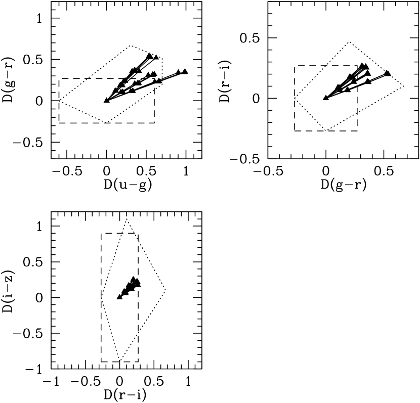
Figure 2.— Reddening vectors in color difference-color difference space are shown by solid lines plus filled triangles. We compute the vectors for the quasar redshift $z_{s}=0.7$, $1.2$, $1.7$, $2.2$, and the lens redshift $z_{s}=0.2$, $0.4$, $0.6$, $0.8$. The differential extinction $\Delta E(B-V)$ is changed from 0 to 0.3 (triangles are plotted every 0.1 increment). The color selections (C1) and (C2) are shown by dashed and dotted boxes, respectively.

We conduct the color selection on the basis of the color difference:

$$D(i-j) = (i-j)_{\rm quasar}-(i-j)_{\rm companion}$$ (4)

$$\;\;{\rm OR}\;\;(i-j)_{\rm companion}-(i-j)_{\rm quasar},$$

where ($i$, $j$)$=$($u$, $g$), ($g$, $r$), ($r$, $i$), ($i$, $z$), and quasar and companion indicate the SDSS spectroscopic quasar in the source quasar sample and candidate companion, respectively. We use PSF magnitudes and their errors throughout the paper. Although the definition of $D(i-j)$ contains a sign ambiguity, we regard candidate pairs as lens candidates if they pass the criteria below using either one of the above definitions: This becomes important when we consider differential reddening, because at first sight we do not know which object is reddened more. When the color difference comes from reddening, $D(i-j)$ for all set of ($i$, $j$) must have the same sign. On the other hand, the color difference of two unrelated objects could have both positive and negative signs for different ($i$, $j$). This is the reason we do not define $D(i-j)$ as the absolute value of the color difference.

Since gravitational lensing does not change the color of objects, the color difference should be small if two components are lensed images of a single quasar. This criterion can be written as follows:

(C1): $$|D(i-j)|<\Delta D(i-j),$$ (5)

which must be met for all four colors. The limit $\Delta D(i-j)$ describes an acceptable error of the color difference, which we adopt the following fixed values

$$\Delta D(u-g) = 3\times 0.20,$$

$$\Delta D(g-r) = 3\times 0.09,$$

$$\Delta D(r-i) = 3\times 0.09,$$

$$\Delta D(i-z) = 3\times 0.30.$$ (6)

These values correspond to typical 3-$\sigma$ errors of the color differences of faint ($\sim 19-20$ mag) objects in the SDSS images. We find that color differences contain very large errors when image separations are small because of the SDSS deblending algorithm. To account for this, we replace $\Delta D(i-j)$ with $3\times\sigma_{D(i-j)}$ for $2^{\prime\prime}\leq\theta<3\farcs 5$, and with $6\times\sigma_{D(i-j)}$ for $\theta\leq 2^{\prime\prime}$, where $\sigma_{D(i-j)}$ is defined by

$$\sigma_{D(i-j)}=\sqrt{(\sigma_{i}^{2}+\sigma_{j}^{2})_{\rm quasar}+(\sigma_{i}^{2}+\sigma_{j}^{2})_{\rm companion}},$$ (7)

where $\sigma_{i}$ are PSF magnitude errors estimated by PHOTO. Since it is quite rare that objects lie at so close to the quasar, the large errors have little effect on the efficiency of our lens selection algorithm.

While gravitational lensing is independent of wavelength, significant color differences between lensed components may be caused by reddening. For instance, Falco et al. (1999) measured the distribution of differential reddening $\Delta E(B-V)$ from a number of gravitationally lensed quasar systems and found that is well described by a Gaussian with a zero mean and standard deviation of $0.1$ mag. We estimate how the differential reddening affects the color difference $D(i-j)$ as follows (see also P03). First, we use the composite quasar spectrum of Vanden Berk et al. (2001) as an input quasar spectral energy distribution. Next we adopt the Galactic extinction law of Cardelli et al. (1989) and compute the color difference as a function of quasar and lens redshifts and $\Delta E(B-V)$, assuming $R_{V}=3.1$. We show estimated reddening vectors for several sets of quasar and lens redshifts in Figure 2. As expected, the effect of the differential reddening is more significant for bluer bands. From this estimation, we prepare another color selection algorithm in color-color space that is designed to select lens systems with large differential reddening:

(C2): $$y>-\frac{\Delta y}{\Delta x}x-\Delta y,$$ (8)

$$y<\frac{y_{2}-y_{1}-\Delta y}{x_{2}-x_{1}+\Delta x}(x-x_{1})+y_{1}+\Delta y,$$

$$y>\frac{y_{2}+\Delta y}{x_{2}+\Delta x}x-\Delta y,$$

$$y<\frac{y_{1}+\Delta y}{x_{1}+\Delta x}(x+\Delta x),$$

$$x<0.2+\Delta x\;\;\;\mbox{IF}\;\;x=D(u-g),$$

where the condition must be satisfied for all set of ($x$, $y$)$=$($D(u-g)$, $D(g-r)$), ($D(g-r)$, $D(r-i)$), ($D(r-i)$, $D(i-z)$), and

$$(x_{1},y_{1},x_{2},y_{2})$$ (12)

$$=\left\{\begin{array}[]{ll}(0.3,0.4,0.4,0.4)&(x,y)=(D(u-g),D(g-r)),\\ (0.2,0.2,0.4,0.1)&(x,y)=(D(g-r),D(r-i)),\\ (0.1,0.2,0.4,0.1)&(x,y)=(D(r-i),D(i-z)).\end{array}\right.$$

The color difference errors, $\Delta x$ and $\Delta y$, were defined in equation (6) and the text that follows it. Figure 2 shows the color selection regions defined by (C1) and (C2). In particular, Figure 2 indicates that the condition (C2) can identify lens systems with very large differential reddening, $\Delta E(B-V)\sim 0.3$. The cut at $D(u-g)=0.2+\Delta D(u-g)$ is added to reduce the contamination of quasar-star pairs. We select quasars that satisfy one or both the criteria (C1) or (C2) as lens candidates.

IV. Testing Selection Algorithm

Figure 3.— The width of PDFs versus sky levels for 1000 randomly selected fields in the SDSS for each band. Open circles indicate those fields that are rejected because of poor seeing.

IV.1. Simulation Method

To quantify the completeness of our selection algorithm, we perform a series of simulations that mimic SDSS observations. We follow the methodology developed by P03, but in this paper we implement multicolor ($ugriz$) simulations to test our selection based both on the morphology and color match.

First, we prepare object fields in which simulated lensed images are placed. We assign the characteristics of each field (sky level, seeing, and magnitude zero-point) from a randomly selected field in the real SDSS data. Figure 3 shows the sky counts and seeing sizes (PSF_WIDTH) of 1000 random fields. Following the discussion in §II, we reject fields with PSF_WIDTH $>1\farcs 8$ in $i$-band in our simulations.

For each field, we also choose a quasar randomly from the subset of the DR3 quasar catalog with $0.6\leq z\leq 2.2$ and $15.0\leq i_{\rm cor}\leq 19.1$, and adopt its redshift and magnitudes in the simulation. However, the redshift and magnitude distributions of the lensed population are quite different from those of the original unlensed population, because the lensing probability is a strong function of redshift and magnitude (e.g., Turner et al., 1984). We account for this difference by assigning to each object a weight proportional to its lensing probability, computed from a singular isothermal sphere model for the mass distribution of lensing galaxies and the velocity function of early-type galaxies derived from the SDSS (Sheth et al., 2003; Mitchell et al., 2005). The velocity function in comoving units is assumed to be constant with redshift. The magnification bias is computed by assuming the luminosity function of quasars obtained from the combination of the Two-Degree Field and SDSS results (Richards et al., 2005, “2SLAQ+Croom et al.” model). Although the lensing probability is sensitive to cosmological parameters, their main effect is to change the overall amplitude of the lensing probability and to have little effect on the dependence of lensing probability on the source redshift and magnitude, on which we are focusing. Figure 4 plots redshifts versus $i$-band magnitudes for randomly selected quasars with and without lensing probability weighting. Because of magnification bias, gravitational lensing preferentially chooses brighter and higher-redshift quasars.

Figure 4.— Redshifts versus $i$-band magnitudes of randomly selected quasars at $0.6\leq z\leq 2.2$ and $15.0\leq i_{\rm cor}\leq 19.1$ are plotted. Open circles are selected from the quasar sample without any weight, and filled triangles used a lensing probability weight.

We convert magnitude to the number of counts with the following equations (Lupton et al., 1999):

$$m=-\frac{2.5}{\ln(10)}\left[{\rm asinh}\left(\frac{F/F_{0}}{2b}\right)+\ln(b)\right],$$ (13)

$$\frac{F}{F_{0}}=\frac{{\rm counts}}{{\rm exptime[sec]}}10^{0.4(Z+kX)},$$ (14)

where $b$ is the softening parameter, $Z$ is the magnitude zero-point, $k$ is the extinction coefficient, $X$ is airmass, and the exposure time is 53.91 sec. Gravitationally lensed images are created in the simulated image by placing two point-source objects that are separated by an angle $\theta$ and have a flux ratio $f_{i}$. For the point-spread function (PSF), we use an analytic PSF composed of two Moffat functions with $\beta_{1}=7$ and $\beta_{2}=2$ and widths given for each field (Racine 1996; P03). The PSF magnitude of each system is normalized to that of the input quasar PSF magnitude in each band. With this procedure, we can simulate lensed quasars with realistic colors and field conditions.

Figure 5.— The distributions of star likelihood star_L for lensed and single quasars, estimated from our simulations. For lensed quasars, we consider only those with objc_type $=6$, image separations $\theta=1^{\prime\prime}-1.4^{\prime\prime}$, and flux ratios $f_{i}>10^{-0.5}$. Vertical dashed lines indicate the limits used in our morphological selection (M1) and (M2) (see §III.1).

We also include differential reddening in our simulation. The value of differential extinction $\Delta E(B-V)$ is randomly distributed as a Gaussian with a standard deviation of $0.1$ mag (Falco et al., 1999). Again, the reddening vectors are computed from the composite quasar spectrum of Vanden Berk et al. (2001) and the extinction curve of Cardelli et al. (1989) assuming $R_{V}=3.1$. The lens redshifts are also assigned randomly in the range $[0.2,z_{\rm max}]$ with $z_{\rm max}={\rm min}(0.8,z_{s}-0.2)$, where $z_{s}$ is the redshift of the source quasar. The distribution has the average redshift $z=0.5$, which is consistent with the value $z\sim 0.51$, the mean of 30 existing gravitationally lensed quasar systems with known lens redshifts. We note the flux ratio $f_{i}$ depends on the band when reddening is included; hereafter we refer to $f_{i}$ as the flux ratio of the $i$-band image.

We next pass these simulated fields through the PHOTO pipeline. Here we briefly summarize the procedure; for more details, see P03. We begin by preparing a PSF frame in which bright PSF stars (constructed from two Moffat functions) are displayed. This PSF field is passed through the fake stamp pipeline and postage stamp pipeline to generate a psField file in which the result of the PSF fit is stored. The object field is passed through the fake stamp pipeline and frames pipeline; this produces tables of the measured object parameters (fpObjc) as well as the cropped atlas images (fpAtlas). We do not need to pass the result through the photometric calibration pipeline, since we can convert counts to magnitudes again by using equations (13) and (14). The magnitude error is estimated from that of the counts as

$$\Delta m=-\frac{2.5}{\ln(10)}\frac{\Delta({\rm counts})}{{\rm exptime[sec]}}\frac{1}{2b}\frac{10^{0.4(Z+kX)}}{\sqrt{1+\left[(F/F_{0})/2b\right]^{2}}}.$$ (15)

The image parameters used to select the lens candidates are extracted from the fpObjc file. When PHOTO deblends two images, we regard the brighter image as targeted by the quasar spectroscopic target selection, and use the image parameters of the brighter image.

We repeat the simulation for different sets of field parameters, redshifts and magnitudes of quasars, and reddening, and compute the completeness of our selection algorithm as a function of the image separation $\theta$ and flux ratio $f_{i}$. Each simulation run consists of simulations of $25\times 21$ quasars; the separation is changed from $0^{\prime\prime}$ to $4\farcs 8$ with a step of $0\farcs 2$ and the flux ratio from $10^{-1}$ to $1$ with a step of a factor of $10^{0.05}$. Since the maximum image separation $\theta=4\farcs 8$ is large enough compare with the seeing sizes of the SDSS images, we think the completenesses of larger-separation lenses can be approximated by those of $\theta=4\farcs 8$. We note that only a few known lensed quasars have the flux ratios $f_{i}<0.1$. We simulate 1000 runs to make an accurate estimation of the completeness.

We note that our simulations differ from those of P03 in several ways. In P03, the selection algorithm was tested for a few choices of seeing sizes and magnitudes of quasars, while in this paper we distributed them in a realistic way. We also simulated images in all five bands, while P03 did not consider differences between different bands.

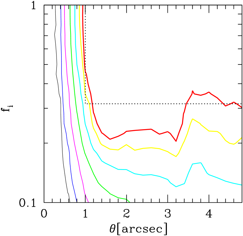
Figure 6.— The completeness of our lens selection algorithm in the image separation $\theta$-flux ratio $f_{i}$ plane, computed from the simulation described in §IV.1. From thick to thin lines, we plot completeness contours of $0.95$, $0.9$, $0.75$, $0.5$, $0.25$, $0.1$, and $0.05$. The dotted lines indicates the limit above which the selection is almost complete.

IV.2. Star Likelihood

Before showing the completeness, we check the distribution of star_L to see the validity of using this parameter to identify lens candidates. All single quasars should be classified as point sources (objc_type $=6$), thus we can choose quite loose conditions for selecting lens candidates, without a significant decrease of efficiency, when they are classified as extended objects (objc_type $=3$; see (M3) in §III.1). Therefore, in this section we concentrate our attention on lenses with objc_type $=6$, for which we need to adopt a good discriminator between lenses and single quasars.

In Figure 5, we show the distributions of star_L in $u$, $g$, $r$, and $i$ for both lensed and single quasars from our simulations. For lensed quasars, we only consider the image separation range of $\theta=1^{\prime\prime}-1.4^{\prime\prime}$ and the flux ratio $f_{i}>10^{-0.5}$. It is clear that the distribution of star_L for lensed quasars is markedly different from that for single quasars. We find that lensed quasars have quite small star likelihoods star_L $\sim 0$ even when lenses are classified as point sources. On the other hand, the distribution of star likelihoods for single quasars peaks at star_L $\sim 1$ and rapidly decreases as star_L decreases. This Figure assures that the conditions (M1) and (M2) presented in §III.1 serve as an excellent method to distinguish gravitational lenses from normal quasars.

IV.3. Completeness

We show the completeness in the $\theta$-$f_{i}$ plane in Figure 6. As expected, lenses with larger image separations and flux ratios closer to unity are more likely to be selected. In particular, our selection algorithm is $\gtrsim 95\%$ complete at $\theta\geq 1^{\prime\prime}$ and $f_{i}\geq 10^{-0.5}$ (indicated by dotted lines). Therefore, we propose to construct a statistical sample within this region of parameter space.

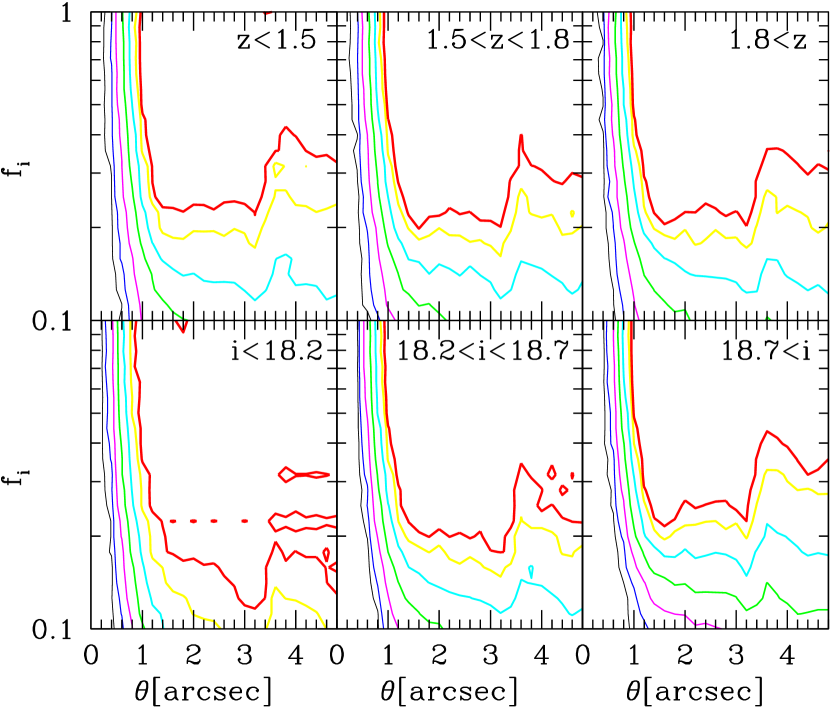
Figure 7.— The completeness of our lens selection algorithm for different redshift and magnitude bins. The definition of lines is same as Figure 6. Upper panels: The completenesses for restricted redshift ranges of $z<1.5$ (left), $1.5<z<1.8$ (center), and $1.8<z$ (right). Lower panels: The completenesses for restricted $i$-band magnitude ranges of $i<18.2$ (left), $18.2<i<18.7$ (center), and $18.7<i$ (right). In both cases, the sizes of bins are determined such that the (lensing probability weighted) number of quasars in each bin becomes roughly equal.

Figure 7 shows the completenesses for three different ranges of redshifts/magnitudes. We find that the completeness is almost independent of the quasar redshift. On the other hand, the completeness shows a weak but significant trend with magnitude, in the sense that brighter quasars are more complete. In particular, the completeness at small $f_{i}$ is larger for brighter quasars. This is reasonable since companion pairs, which are often hidden when $f_{i}$ is small, are more easily detected for brighter quasars. However, even for faintest quasars ($i>18.7$) the completeness at $\theta\geq 1^{\prime\prime}$ and $f_{i}\geq 10^{-0.5}$ is very high. Therefore we conclude that our selection does not affect the distributions of redshifts and magnitudes of lensed quasars very much.

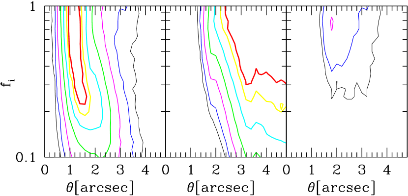
Figure 8.— Left: The completeness of the morphological selection only. Center: The completeness of the color selection only. Right: The fraction of lenses selected from both morphological and color selections. The definition of lines is same as Figure 6.

Table 1Completeness for double lenses

$\log(f_{i})$	$\theta$	Completeness
	[arcsec]	total	morph	color	both
$-1.00$	0.0	0.036	0.036	0.000	0.000
$-1.00$	0.2	0.031	0.031	0.000	0.000
$-1.00$	0.4	0.032	0.032	0.000	0.000
$-1.00$	0.6	0.041	0.041	0.000	0.000
$-1.00$	0.8	0.100	0.100	0.000	0.000
$-1.00$	1.0	0.213	0.213	0.000	0.000
$-1.00$	1.2	0.304	0.304	0.000	0.000
$-1.00$	1.4	0.378	0.378	0.000	0.000
$-1.00$	1.6	0.415	0.415	0.001	0.001
$-1.00$	1.8	0.461	0.459	0.005	0.003
$-1.00$	2.0	0.472	0.463	0.011	0.002

Note. — Full table to appear in the on-line edition.

Figure 6 does not make it clear if lenses are mainly chosen by the morphological or color selection at each point in the $\theta$-$f_{i}$ plane. Figure 8 shows the completeness from the two selection algorithms separately. We also show the overlap of these two selections. At $\theta\lesssim 2^{\prime\prime}$ lenses are mostly selected morphologically, and at $\theta\gtrsim 2^{\prime\prime}$ the color selection dominates. The overlap of these two selections is quite small. The completeness from the two selection algorithms as well as total completeness are listed in Table 1.

IV.4. Magnification Factor

The magnification bias is one of the most important elements in predicting lensing probabilities. The SDSS quasar target selection (Richards et al., 2002) uses PSF magnitudes for the magnitude limit, therefore we examine those of simulated lensed quasars with various image separations. Basically, when the image separation is quite large and two images are deblended successfully by PHOTO, the PSF magnitude of the targeted quasar should be roughly equal to that of the brighter image. However, when the image separation is too small to be distinguished from a point source, the PSF magnitude is that of the sum of the two images. Bearing this in mind, we define the following parameter:

$$\bar{\mu}\equiv\frac{\mu-\mu_{\rm bri}}{\mu_{\rm fai}},$$ (16)

where $\mu_{\rm bri}$ and $\mu_{\rm fai}$ are the magnification factors for the brighter and fainter images, respectively. The magnification factor $\mu$ indicates the one measured in the SDSS (i.e., the PSF magnitude of the lens system divided by the original magnitude of the source quasar). The definition indicates that $\mu=\mu_{\rm tot}\equiv\mu_{\rm bri}+\mu_{\rm fai}$ and $\mu=\mu_{\rm bri}$ correspond to $\bar{\mu}=1$ and $\bar{\mu}=0$, respectively. Therefore, the parameter should approach zero at large separations, and $\bar{\mu}\rightarrow 1$ for $\theta\rightarrow 0$.

Figure 9.— The magnification factor of lensed quasars. The parameter $\bar{\mu}$ (eq. [16]) is plotted as a function of image separation $\theta$. For each image separation the mean and its standard deviation are shown. The dashed line indicates the analytic fit (eq. [17]).

We derive $\bar{\mu}$ as a function of the image separation from our simulation runs. We only consider simulated lens systems with flux ratio $f_{i}\geq 10^{-0.5}$, because the derived $\bar{\mu}$ contains large errors when flux ratios are very large $\mu_{\rm bri}\gg\mu_{\rm fai}$, and also because the completeness is low for large flux ratio systems. Moreover, $\mu_{\rm tot}\sim\mu_{\rm bri}$ at $f_{i}\ll 1$ implies that the magnification factors do not change as a function of the image separation in any case. Figure 9 plots the result. As expected, $\bar{\mu}$ changes from $\bar{\mu}\sim 1$ to $\sim 0$ with increasing image separations. We find that the curve is fitted roughly by the following form:

$$\bar{\mu}=\frac{1}{2}\left[1+\tanh\left(1.76-1.78\theta\right)\right],$$ (17)

where the image separation $\theta$ is in units of arcsec.

We note that for a given image separation the magnification bias can be written as

$$B=\bar{\mu}B_{\rm tot}+(1-\bar{\mu})B_{\rm bri},$$ (18)

where $B_{\rm tot}$ and $B_{\rm bri}$ are the magnification bias from the total magnification and magnification of the brighter image, respectively.

IV.5. Quadruple Lens Systems

Table 2Quadruply lensed quasars used in the simulation

Name	Typea	$\theta$b	$f_{\rm quad}$c	Referenced
PG 1115+080	fold	$2\farcs 43$	0.17	CASTLESe
SDSS J0924+0129	fold	$1\farcs 81$	0.47	Keeton et al. (2006)
SDSS J1004+4112	fold	$14\farcs 6$	0.23	Oguri et al. (2004a)
WFI2026$-$4536	fold	$1\farcs 44$	0.31	Morgan et al. (2004)
WFI2033$-$4723	fold	$2\farcs 53$	0.56	Morgan et al. (2004)
HE0230$-$2130	fold	$2\farcs 19$	0.59	CASTLESe
MG0414+0534	fold	$2\farcs 13$	0.47	CASTLESe
B0712+472	fold	$1\farcs 29$	0.20	CASTLESe
B1555+375	fold	$0\farcs 42$	0.49	Marlow et al. (1999)
B1608+656	fold	$2\farcs 10$	0.49	Fassnacht et al. (2002)
H1413+117	cross	$1\farcs 35$	0.71	CASTLESe
HE0435$-$1223	cross	$2\farcs 56$	0.62	Wisotzki et al. (2002)
HST12531$-$2914	cross	$1\farcs 38$	0.92	CASTLESe
HST14113+5211	cross	$2\farcs 26$	0.82	CASTLESe
HST14176+5226	cross	$3\farcs 26$	0.79	CASTLESe
Q2237+030	cross	$1\farcs 83$	0.31	CASTLESe
RX J0911+0551	cusp	$3\farcs 25$	0.31	CASTLESe
RX J1131$-$1231	cusp	$3\farcs 24$	0.09	Sluse et al. (2003)
B0128+437	cusp	$0\farcs 55$	0.53	Phillips et al. (2000)
B1422+231	cusp	$1\farcs 29$	0.03	CASTLESe

Based on visual inspection. The maximum separation between multiple images. The flux ratio between the brightest image and the image farthest from the brightest image. The reference from which we adopt the image positions and fluxes for the simulation. For fluxes, we use those of the $i$-band (F814W for the Hubble Space Telescope data) image when the optical data are available. If not, we adopt those of the radio band image. C. S. Kochanek, E. E. Falco, C. Impey, J. Lehar, B. McLeod, H.-W. Rix, CASTLES survey, http://cfa-www.harvard.edu/castles/

Thus far we have concentrated our attention on two-component lenses, but in reality a non-negligible fraction of gravitationally lensed quasars have four components. In this subsection we consider our selection algorithm’s effectiveness for such quadruple lenses.

The difficulty in studying the selection of quadruple lenses lies in their complexity; while double lenses are parameterized by flux ratio and image separation, we require 8 parameters to characterize a quadruple lens, making a full exploration almost impossible. Instead, in this paper we adopt the image configurations and flux ratios from 20 known quadruple lenses taken from the CASTLES webpage (see Table 2). We apply a similarity transformation to the quadruple lenses in order to derive the completeness as a function of the image separation. We define the image separation to be the maximum distance between multiple images. The differential reddening is included, again using the distribution of Falco et al. (1999). As in the case of double lenses, we simulate 1000 runs to make an accurate estimate of the completeness.

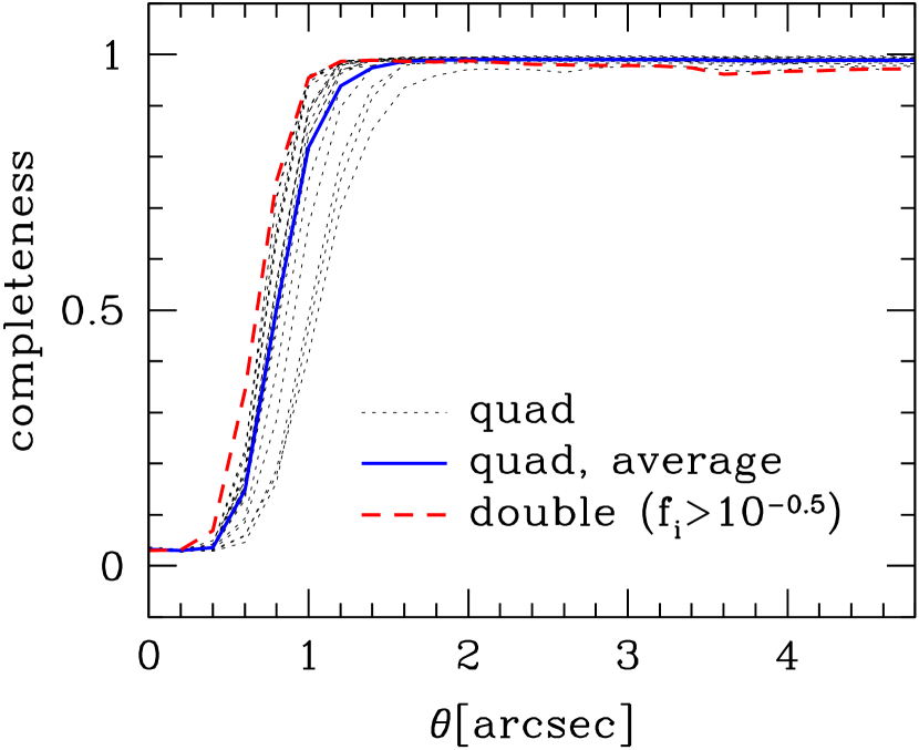
Figure 10.— The completeness for quadruple lenses as a function of the image separation. The dotted line shows the completeness of each quadruple lens image configuration and flux ratios taken from real observational data (see Table 2). The thick solid line indicates the completeness averaged over the 20 dotted lines. The completeness of double lenses, averaged over the flux ratios in the range $10^{-0.5}<f_{i}<1$, is also shown for reference.

Figure 10 plots the completeness of each of the 20 quadruple lens configurations as a function of the image separation, as well as the average of them. We find that our algorithm can select quadruple lenses reasonably well: Even in the limiting case, $\theta=1^{\prime\prime}$, the completeness is $82\%$ on average, and at $\theta>2^{\prime\prime}$ it is almost unity. We note that in both cases the completenesses vary most rapidly at $\theta\sim 1^{\prime\prime}$ where the number of lensed quasars peaks. There is a systematic difference of the completeness between double and quadruple lenses: At $\theta<2^{\prime\prime}$ the completeness for double lenses is larger than that for quadruple lenses, while at $\theta>2^{\prime\prime}$ the quadruple lenses are more complete. The differences are small, but they might become important when discussing the relative number of quadruple and double lenses (Keeton et al., 1997; Rusin & Tegmark, 2001; Chae, 2003; Oguri & Keeton, 2004).

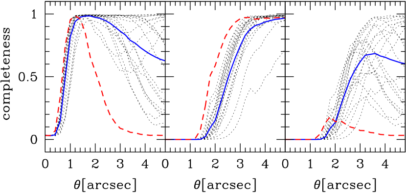
Figure 11.— The completeness for quadruple lenses, with the morphological selection only (left), the color selection only (center), and both morphological and color selections (right). The definition of lines is same as in Figure 10.

Figure 11 shows the completeness for morphological and color selections separately. Unlike double lenses, quadruple lenses are effectively chosen by the morphological selection even at large image separations, $\theta>3^{\prime\prime}$. In addition, it is quite common that lenses are selected by both criteria This is because quadruple lenses are more complex than double lenses. In particular, the complexity and larger number of images for quadruple lenses make the completeness at $\theta>2^{\prime\prime}$ quite large. Again, the completeness from the two selection algorithms as well as total completeness are listed in Table 3.

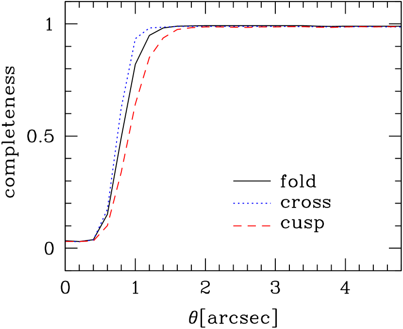
Figure 12.— The completeness for quadruple lenses of different image configuration types: fold (solid) , cross (dotted), and cusp (dashed).

We also study the completeness for different image configuration types: fold (two of the images lie close together), cross (almost symmetric), and cusp (three of the images lie close together). To do so, we divide the 20 quadruple lenses into these three categories by visual inspection, and compute the average completeness for each category. The categorization is summarized in Table 2, and the results are shown in Figure 12. Our algorithm selects cross lenses very well, but is less effective for cusp lenses; this is because the fourth image of a cusp lens, which lies far from the critical curve, is usually much fainter than the other images near the critical curve and therefore the effective “flux ratio” of cusp lenses becomes small. To pursue this further, we consider the flux ratio between the brightest image and the image farthest from the brightest image (denoted by $f_{\rm quad}$), and see its correlation with the completeness. Figure 13 plots $f_{\rm quad}$ and the completeness at $\theta=1^{\prime\prime}$ for all 20 quadruple lenses listed in Table 2. As expected, we see a clear correlation: All quadruple lenses with completeness $<0.8$ have $f_{\rm quad}<0.4$. Therefore, despite the complexity and large number of parameters involved in quadruple lenses, $f_{\rm quad}$ gives a rough criterion of how well our selection algorithm can identify quadruple lenses.

Figure 13.— The completeness at $\theta=1^{\prime\prime}$ and $f_{\rm quad}$ (the flux ratio between the brightest image and the image farthest from the brightest image) for 20 known quadruple lenses. The values of $f_{\rm quad}$ are listed in Table 2.

Table 3Completeness for quadruple lenses

Name	$\theta$	Completeness
	[arcsec]	total	morph	color	both
PG1115+080	0.0	0.035	0.035	0.000	0.000
PG1115+080	0.2	0.030	0.030	0.000	0.000
PG1115+080	0.4	0.029	0.029	0.000	0.000
PG1115+080	0.6	0.059	0.059	0.000	0.000
PG1115+080	0.8	0.188	0.188	0.000	0.000
PG1115+080	1.0	0.490	0.490	0.000	0.000
PG1115+080	1.2	0.796	0.796	0.000	0.000
PG1115+080	1.4	0.937	0.937	0.000	0.000
PG1115+080	1.6	0.978	0.978	0.001	0.001
PG1115+080	1.8	0.987	0.987	0.007	0.007
PG1115+080	2.0	0.992	0.991	0.016	0.015

Note. — Full table to appear in the on-line edition.

V. Removing Single Quasars

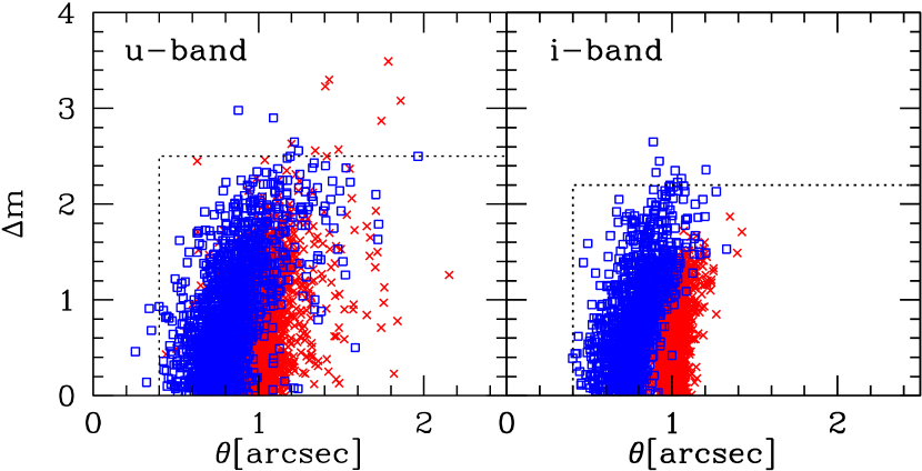
Figure 14.— The distribution of inferred magnification differences ($\Delta m$) and image separation ($\theta$) of simulated images, derived from fitting by two PSFs with GALFIT software (Peng et al., 2002). The true image separation and the $i$-band flux ratio are set to $\theta=1^{\prime\prime}$ and $f_{i}=[10^{-0.5},1]$ (for double lenses), respectively. Crosses indicate double lenses, and open squares are quadruple lenses. The left and right panels show the results of $u$-band and $i$-band images, respectively. The dotted lines indicate our proposed limit in the image separation-flux ratio space (S1) defined in equation (19).

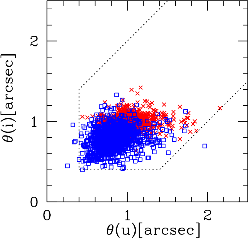
Figure 15.— The distribution of $u$- and $i$-band image separations ($\theta$) of simulated images with $\theta=1^{\prime\prime}$ and the $i$-band flux ratio $f_{i}=[10^{-0.5},1]$ (for double lenses), derived from fitting by two PSFs with GALFIT software (Peng et al., 2002). Crosses indicate double lenses, and open squares are quadruple lenses. The dotted lines indicate our proposed limit in the image separation space (S1) defined in equation (19).

The nonzero completeness at $\theta\rightarrow 0$ implies that our morphological selection algorithm falsely identifies “normal” quasars as lenses. Indeed, when we apply our algorithm to DR3 quasar catalog, we find many lens candidates, many of which appear to be point sources (see §VI), although most normal single quasars are removed by our morphological selection. Therefore, in this section, we present an additional selection which is aimed to exclude such point sources.

To do so, we fit systems selected by our morphological selection algorithm with two PSFs using the GALFIT package (Peng et al., 2002), and derive the image separation and flux ratio. We use stars in the same field as a PSF template in fitting. The fitting of any single object with two PSFs should result in either too large magnitude differences or too small image separations. Here we only consider gravitational lenses included in the proposed statistical sample, i.e., those with $\theta>1^{\prime\prime}$ and $f_{i}>10^{-0.5}$. The point sources should have significantly smaller image separation and/or larger flux ratios than the above limit. Therefore we can reject such point sources by making a cut in image separation-flux ratio space. We do this fit on both the $u$- and $i$-band images: We use the $i$-band image because the flux ratio is defined by that of the $i$-band image. The $u$-band is used because it is a powerful discriminator between lensed pairs and superpositions of quasars and stars or quasars and galaxies.

To determine the region of parameter space we should exclude, we perform fitting of simulated images (see §IV.1). We consider only the extreme image separation, $\theta=1^{\prime\prime}$, for which fitting by two PSFs will be most difficult. The flux ratio varied over the range $f_{i}=[10^{-0.5},1]$. We show the results for both $u$- and $i$-band simulated images in Figures 14 (distribution in image separation-flux ratio space for each band) and 15 (distribution in $u$- and $i$-band image separation space). It is seen that quadruple lenses show smaller image separations on average than double lenses; this is clearly because GALFIT tends to fit the two brightest images that are not necessarily the two separated farthest from each other. From this result, we determine the selection criterion to be the following:

(S1): $$\theta(u)\geq 0\farcs 4,$$ (19)

$$\theta(i)\geq 0\farcs 4,$$

$$\Delta m(u)\leq 2.5,$$

$$\Delta m(i)\leq 2.2,$$

$$\left|\theta(u)-\theta(i)\right|\leq 1^{\prime\prime},$$

where $\theta$ and $\Delta m$ are the separation and magnitude difference between fitted two PSF components. We select candidates that meet all of the above criteria. In our simulation, more than 99% of double and quadruple lenses with $\theta=1^{\prime\prime}$ pass the condition, thus we conclude that this additional selection hardly changes the high completeness of our statistical lens sample estimated in §IV. The condition (S1) rejects $\sim 85\%$ of candidates selected by the morphological selection (see §VI).

VI. Efficiency

A definitive estimate of the efficiency requires follow-up observations of all candidates which is still in progress. Nevertheless, in this section we discuss the efficiency of our selection algorithm in light of the follow-up observations that we have performed thus far.

Table 4Preliminary efficiency of our selection algorithm

$\theta$	$N_{\rm mor}$a	$N_{\rm mor+}$b	$N_{\rm col}$c	$N_{\rm cand}$d	$N_{\rm obs}$e	$N_{\rm lens}$f	$N_{\rm lens}/N_{\rm cand}$
$<2^{\prime\prime}$	568	88	9	96	77	8	0.083
$2^{\prime\prime}-7^{\prime\prime}$	74	8	59	66	62	2	0.030
$7^{\prime\prime}-20^{\prime\prime}$	6	0	155	155	141	1	0.006
$<20^{\prime\prime}$	648	96	223	317	280	11	0.035

Number of candidates selected by the morphological selection. Number of candidates selected by the morphological selection plus additional selection presented in §V. Number of candidates selected by the color selection. Total number of candidates selected by the morphological and color selection. It does not necessarily coincide with the sum of $N_{\rm mor+}$ and $N_{\rm col}$, because some of candidates are selected by both algorithms. Number of candidates for which judgement of lens/nonlens was made on the basis of follow-up observations and/or various survey data. Current number of confirmed lenses included among the candidates.

To do so, we again adopt the DR3 quasar sample (Schneider et al., 2005). As discussed in §II, we use 22,682 quasars at $0.6\leq z\leq 2.2$ and $15.0\leq i_{\rm cor}\leq 19.1$ as our source quasar sample. We apply our algorithms to the quasar sample, and select $648$ candidates from the morphological selection and $228$ candidates from the color selection. By applying the additional cut described in §V to morphologically selected candidates, the number of candidates from the morphological selection reduces to $97$, only $\sim 15$% of the original. For color selection, we only selected candidates with image separations smaller than $20\farcs 1$ and magnitude differences smaller than $1.3$, since we concentrate our attention to the lens sample in the range $1^{\prime\prime}\leq\theta\leq 20^{\prime\prime}$ and $f_{i}\geq 10^{-0.5}$. It is expected that the efficiency is a strong function of the image separation, thus we consider the three image separation ranges, $\theta<2^{\prime\prime}$, $2^{\prime\prime}<\theta<7^{\prime\prime}$, and $7^{\prime\prime}<\theta$, and derive the efficiency for each image separation range separately. The image separations of morphologically selected candidates we used are those obtained by fitting $i$-band SDSS images with two PSFs using GALFIT (see §V). The result is summarized in Table 4. We note that the algorithm successfully identified all known lenses included in the subset of the DR3 quasar catalog, thereby confirming the high completeness shown in §IV. Since we still have candidates that are to be observed, the efficiency shown in Table 4 should in principle be regarded as the lower limit. However, we believe that this is close to the true value because of the “observation bias” whereby we preferentially observe better candidates. As expected, the efficiency is dependent on the image separation: The efficiencies are 8%, 3%, and 0.6% for $\theta<2^{\prime\prime}$, $2^{\prime\prime}<\theta<7^{\prime\prime}$, and $7^{\prime\prime}<\theta$, respectively. Most false positives, which have been revealed by follow-up observations, were quasar-star pairs or quasar pairs (see also Hennawi et al., 2006a). For the smallest image separation bin, the efficiency is comparable to that of the CLASS, which discovered 13 gravitational lenses out of 149 candidates (Browne et al., 2003). We note that the candidates can be restricted further by comparing with other existing observations (see Paper II) such as Faint Images of the Radio Sky at Twenty-cm (Becker et al., 1995), which should increase the efficiency.

VII. Conclusion

We have presented the SQLS lens candidate selection algorithm from the SDSS spectroscopic quasar catalog. Our algorithm consists of two selection methods, a morphological selection that identifies “extended” quasars, and a color selection that picks up adjacent objects with similar colors. Both selection methods rely only on imaging parameters that the SDSS reduction pipeline generates, thereby allowing easy and fast selection of lens candidates. To reduce the number of candidates further, we fit the images of morphologically selected candidates with two PSFs, deriving the image separations and magnitude differences, and applying cuts in the image separation-magnitude difference space. This allows us to remove most single quasars that are otherwise selected by the morphological selection.

We have performed simulations of lensed quasar images in the SDSS to determine the effectiveness of the selection algorithm. In the simulations, distributions of field parameters (i.e., seeings and sky levels) as well as those of source quasars are taken from the real SDSS data. We have also taken differential reddening by lens galaxies into account. The simulated SDSS images are then passed through the imaging data processing pipeline used in the SDSS. This allows a reliable estimate of the completeness of the algorithm to be made. We have found that our selection algorithm is almost complete at image separations larger than $1^{\prime\prime}$ and flux ratios larger than $10^{-0.5}$. We have also quantified the magnification factor of lensed images as a function of the image separation, which is important for accurate computation of magnification bias. The algorithm successfully identifies both double and quadruple lenses, although there is a systematic difference of completenesses between double and quadruple lenses. The efficiency depends strongly on the image separation; at separations less than $2^{\prime\prime}$ the preliminary efficiency of our selection algorithm is about 8%, comparable to that of the CLASS.

An important effect we have neglected in our simulation is fluxes from lens galaxies. Although for quasars with $i\lesssim 19.1$ and redshifts above $0.6$ lens galaxies tend to be fainter than lensed quasars, they could affect quantitative results. An important point is that lensed quasars are not selected by the quasar spectroscopic target selection if the fluxes of lens galaxies dominate: A good example is the high-redshift lens SDSS J0903+5028 (Johnston et al., 2003) that was targeted for SDSS spectroscopy as a luminous red galaxy, rather than a quasar, because the lensing galaxy is brighter than the lensed quasar images. Therefore such systems will not be included in SDSS spectroscopic quasar catalogs. This means that we need to simulate quasar spectroscopic target selection for lensed systems, as well as lens selection algorithms, to address the effect of lens galaxy fluxes. This is beyond the scope of this paper.

The well-understood selection function, together with the knowledge of redshift and magnitude distributions of source quasars, is very important to control possible systematic effects. We plan to construct a first SQLS complete lens sample from the DR3 quasar catalog, which will be presented in Paper II.

Appendix A Object types of lensed quasar systems

Gravitationally lensed quasars are sometimes classified as extended objects (objc_type $=3$) by PHOTO. This is very important for lensing of high-redshift ($z\gtrsim 3$) quasars because extended high-redshift quasars are not targeted by the quasar target selection pipeline (see Figure 1). Therefore, we need to take this bias into account when we constrain the shape of the high-redshift quasar luminosity function from the absence of strong gravitational lensing (e.g., Richards et al., 2006a). In addition, this bias strongly affects the search for lenses using a photometrically selected quasar sample (Richards et al., 2004), because extended quasars are not included in the photometric sample, again in order to enhance the efficiency. In this appendix, we derive the fraction of lens systems that are classified as extended objects from our simulations of lensed quasar images (§IV). Although we focused our attention on bright ($i<19.1$) low-redshift quasars and therefore the result may not be applied to high-redshift quasars that are fainter and have quite different colors, the result is still useful to understand how PHOTO classifies lensed quasar images.

Figure 16 shows the fraction of double lenses that are classified as extended objects in the $\theta$-$f_{i}$ plane. As expected, the fraction is a strong function of the image separation: The lenses with $\theta\sim 1\farcs 2$ are most likely judged as extended objects. The fraction depends on the flux ratio; lenses with larger $f_{i}$ are more likely to be classified as extended objects. In Figure 17 we plot the same fraction for quadruple lenses. Although the system-by-system difference is large, at $\theta\gtrsim 1\farcs 5$ quadruple lenses are more likely to be classified as extended objects on average than double lenses, which is clearly because the existence of close fold/cusp image pairs.

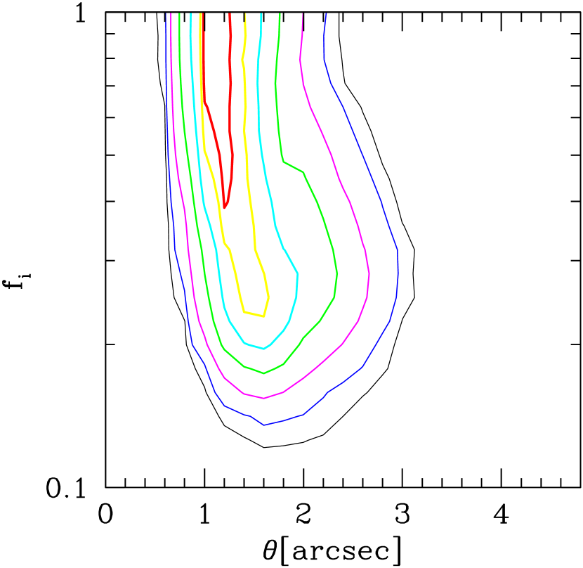
Figure 16.— Contours of the fraction of simulated double lenses that are classified as extended objects (objc_type $=3$). The definition of lines is same as in Figure 6.

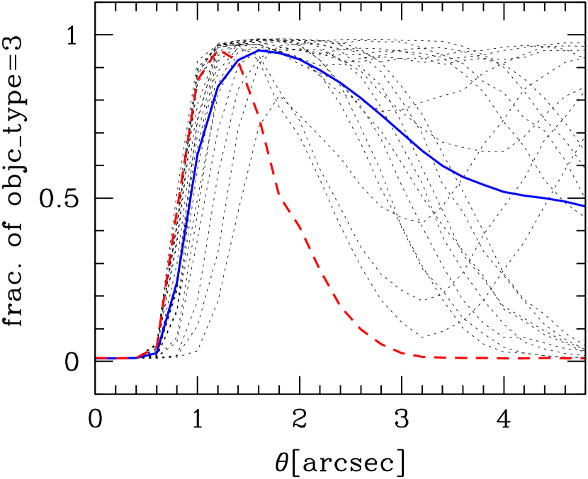
Figure 17.— The fraction of quadruple lenses that are classified as extended objects (objc_type $=3$). The dotted line shows the fraction of each quadruple lens image configuration and flux ratios taken from real observational data (see Table 2), while the thick solid line indicates the fraction averaged over the 20 dotted lines. The fraction for double lenses, averaged over the flux ratios in the range $10^{-0.5}<f_{i}<1$, is also shown by a dashed line for reference.

References

- Abazajian et al. (2003) Abazajian, K., et al. 2003, AJ, 126, 2081
- Abazajian et al. (2004) Abazajian, K., et al. 2004, AJ, 128, 502
- Abazajian et al. (2005) Abazajian, K., et al. 2005, AJ, 129, 1755
- Adelman-McCarthy et al. (2006) Adelman-McCarthy, J. K., et al. 2006, ApJS, 162, 38
- Becker et al. (1995) Becker, R. H., White, R. L., & Helfand, D. J. 1995, Astrophys. J. , 450, 559
- Blanton et al. (2003) Blanton, M. R., Lin, H., Lupton, R. H., Maley, F. M., Young, N., Zehavi, I., & Loveday, J. 2003, AJ, 125, 2276
- Bolton et al. (2005) Bolton, A. S., Burles, S., Koopmans, L. V. E., Treu, T., & Moustakas, L. A. 2005, ApJ, 624, L21
- Bolton et al. (2006) Bolton, A. S., Burles, S., Koopmans, L. V. E., Treu, T., & Moustakas, L. A. 2006, Astrophys. J. , 638, 703
- Browne et al. (2003) Browne, I. W. A., et al. 2003, MNRAS, 341, 13
- Burles et al. (2006) Burles, S., et al. 2006, AJ, in preparation
- Cardelli et al. (1989) Cardelli, J. A., Clayton, G. C., & Mathis, J. S. 1989, Astrophys. J. , 345, 245
- Chae (2003) Chae, K.-H. 2003, MNRAS, 346, 746
- Chiba & Yoshii (1999) Chiba, M., & Yoshii, Y. 1999, Astrophys. J. , 510, 42
- Dalal & Kochanek (2002) Dalal, N., & Kochanek, C. S. 2002, Astrophys. J. , 572, 25
- Eisenstein et al. (2001) Eisenstein, D. J., et al. 2001, AJ, 122, 2267
- Falco et al. (1999) Falco, E. E., et al. 1999, Astrophys. J. , 523, 617
- Fassnacht et al. (2002) Fassnacht, C. D., Xanthopoulos, E., Koopmans, L. V. E., & Rusin, D. 2002, Astrophys. J. , 581, 823
- Fukugita et al. (1990) Fukugita, M., Futamase, T., & Kasai, M. 1990, MNRAS, 246, 24P
- Fukugita et al. (1996) Fukugita, M., Ichikawa, T., Gunn, J. E., Doi, M., Shimasaku, K., & Schneider, D. P. 1996, AJ, 111, 1748
- Gunn et al. (1998) Gunn, J. E., et al. 1998, AJ, 116, 3040
- Gunn et al. (2006) Gunn, J. E., et al. 2006, AJ, 131, 2332
- Hennawi et al. (2006a) Hennawi, J. F., et al. 2006a, AJ, 131, 1
- Hennawi et al. (2006b) Hennawi, J. F., Dalal, N., Bode, P., & Ostriker, J. P. 2006b, Astrophys. J. , submitted (astro-ph/0506171)
- Hogg et al. (2001) Hogg, D. W., Finkbeiner, D. P., Schlegel, D. J., & Gunn, J. E. 2001, AJ, 122, 2129
- Hopkins et al. (2004) Hopkins, P. F., et al. 2004, AJ, 128, 1112
- Inada et al. (2003a) Inada, N., et al. 2003a, AJ, 126, 666
- Inada et al. (2003b) Inada, N., et al. 2003b, AJ, submitted
- Inada et al. (2003c) Inada, N., et al. 2003c, Nature (London), 426, 810
- Inada et al. (2005) Inada, N., et al. 2005, AJ, 130, 1967
- Inada et al. (2006) Inada, N., et al. 2006, AJ, 131, 1934
- Ivezić et al. (2004) Ivezić, Ž., et al. 2004, AN, 325, 583
- Johnston et al. (2003) Johnston, D. E., et al. 2003, AJ, 126, 2281
- Keeton et al. (1997) Keeton, C. R., Kochanek, C. S., & Seljak, U. 1997, Astrophys. J. , 482, 604
- Keeton et al. (2006) Keeton, C. R., Burles, S., Schechter, P. L., & Wambsganss, J. 2006, Astrophys. J. , 639, 1
- Kochanek (1996) Kochanek, C. S. 1996, Astrophys. J. , 466, 638
- Kochanek & White (2001) Kochanek, C. S., & White, M. 2001, Astrophys. J. , 559, 531
- Lupton et al. (1999) Lupton, R. H., Gunn, J. E., & Szalay, A. S. 1999, AJ, 118, 1406
- Lupton et al. (2001) Lupton, R., Gunn, J. E., Ivezić, Z., Knapp, G. R., Kent, S., & Yasuda, N. 2001, in ASP Conf. Ser. 238, Astronomical Data Analysis Software and Systems X, ed. F. R. Harnden, Jr., F. A. Primini, and H. E. Payne (San Francisco: Astr. Soc. Pac.), p. 269 (astro-ph/0101420)
- Maoz et al. (1997) Maoz, D., Rix, H.-W., Gal-Yam, A., & Gould, A. 1997, Astrophys. J. , 486, 75
- Marlow et al. (1999) Marlow, D. R., et al. 1999, AJ, 118, 654
- Mitchell et al. (2005) Mitchell, J. L., Keeton, C. R., Frieman, J. A., & Sheth, R. K. 2005, Astrophys. J. , 622, 81
- Morgan et al. (2003) Morgan, N. D., Snyder, J. A., & Reens, L. H. 2003, AJ, 126, 2145
- Morgan et al. (2004) Morgan, N. D., Caldwell, J. A. R., Schechter, P. L., Dressler, A., Egami, E., & Rix, H.-W. 2004, AJ, 127, 2617
- Myers et al. (2003) Myers, S. T., et al. 2003, MNRAS, 341, 1
- Narayan & White (1988) Narayan, R., & White, S. D. M. 1988, MNRAS, 231, 97P
- Oguri et al. (2004a) Oguri, M., et al. 2004a, Astrophys. J. , 605, 78
- Oguri et al. (2004b) Oguri, M., et al. 2004b, PASJ, 56, 399
- Oguri & Keeton (2004) Oguri, M., & Keeton, C. R. 2004, Astrophys. J. , 610, 663
- Oguri et al. (2005a) Oguri, M., et al. 2005a, Astrophys. J. , 622, 106
- Oguri et al. (2005b) Oguri, M., Keeton, C. R., & Dalal, N. 2005b, MNRAS, 364, 1451
- Oguri (2006) Oguri, M. 2006, MNRAS, 367, 1241
- Peng et al. (2002) Peng, C. Y., Ho, L. C., Impey, C. D., & Rix, H.-W. 2002, AJ, 124, 266
- Phillips et al. (2000) Phillips, P. M., et al. 2000, MNRAS, 319, L7
- Pier et al. (2003) Pier, J. R., Munn, J. A., Hindsley, R. B., Hennessy, G. S., Kent, S. M., Lupton, R. H., & Ivezić, Ž. 2003, AJ, 125, 1559
- Pindor et al. (2003) Pindor, B., Turner, E. L., Lupton, R. H., & Brinkmann, J. 2003, AJ, 125, 2325 (P03)
- Pindor et al. (2004) Pindor, B., et al. 2004, AJ, 127, 1318
- Pindor et al. (2006) Pindor, B., et al. 2006, AJ, 131, 41
- Racine (1996) Racine, R. 1996, PASP, 108, 699
- Richards et al. (2002) Richards, G. T., et al. 2002, AJ, 123, 2945
- Richards et al. (2003) Richards, G. T., et al. 2003, AJ, 126, 1131
- Richards et al. (2004) Richards, G. T., et al. 2004, ApJS, 155, 257
- Richards et al. (2005) Richards, G. T., et al. 2005, MNRAS, 360, 839
- Richards et al. (2006a) Richards, G. T., et al. 2006a, AJ, 131, 49
- Richards et al. (2006b) Richards, G. T., et al. 2006b, AJ, in press (astro-ph/0601434)
- Rusin & Tegmark (2001) Rusin, D., & Tegmark, M. 2001, Astrophys. J. , 553, 709
- Rusin & Kochanek (2005) Rusin, D., & Kochanek, C. S. 2005, Astrophys. J. , 623, 666
- Schlegel et al. (1998) Schlegel, D. J., Finkbeiner, D. P., & Davis, M. 1998, Astrophys. J. , 500, 525
- Schneider et al. (2002) Schneider, D. P., et al. 2002, AJ, 123, 567
- Schneider et al. (2003) Schneider, D. P., et al. 2003, AJ, 126, 2579
- Schneider et al. (2005) Schneider, D. P., et al. 2005, AJ, 130, 367
- Sheth et al. (2003) Sheth, R. K., et al. 2003, Astrophys. J. , 594, 225
- Sluse et al. (2003) Sluse, D., et al. 2003, A&A, 406, L43
- Smith et al. (2002) Smith, J. A., et al. 2002, AJ, 123, 2121
- Stoughton et al. (2002) Stoughton, C., et al. 2002, AJ, 123, 485
- Strauss et al. (2002) Strauss, M. A., et al. 2002, AJ, 124, 1810
- Treu & Koopmans (2004) Treu, T., & Koopmans, L. V. E. 2004, Astrophys. J. , 611, 739
- Turner (1990) Turner, E. L. 1990, ApJ, 365, L43
- Turner et al. (1984) Turner, E. L., Ostriker, J. P., & Gott, J. R. 1984, Astrophys. J. , 284, 1
- Vanden Berk et al. (2001) Vanden Berk, D. E., et al. 2001, AJ, 122, 549
- Wisotzki et al. (2002) Wisotzki, L., Schechter, P. L., Bradt, H. V., Heinmüller, J., & Reimers, D. 2002, A&A, 395, 17
- York et al. (2000) York, D. G., et al. 2000, AJ, 120, 1579