Fast kink modes of longitudinally stratified coronal loops

Abstract

Aims. We investigate the standing kink modes of a cylindrical model of coronal loops. The density is stratified along the loop axis and changes discontinuously at the surface of the cylinder. The periods and mode profiles are studies with their deviation from those of the unstratified loops. The aim is to extract information on the density scale heights prevailing in the solar corona.

Methods. The problem is reduced to solving a single second-order partial differential equation for $\delta B_{z}(r,z)$, the longitudinal component of the Eulerian perturbations of the magnetic field. This equation, in turn, is separated into two second-order ordinary, differential equations in $r$ and $z$ that are, however, connected through a dispersion relation between the frequencies and the longitudinal wave numbers. In the thin tube approximation, the eigensolutions are obtained by a perturbation technique, where the perturbation parameter is the density stratification parameter. Otherwise the problem is solved numerically.

Results. 1) On functional dependencies of the dispersion relation the radial wave number is independent of the longitudinal stratification. 2) We verify the earlier computational finding that the first overtone frequencies increase with increasing stratification and the observational finding (from analysis of TRACE data) that the ratio of the first to the fundamental overtone frequency decreases with increasing stratification. The method we use to arrive at these conclusions, however, is more analytical than computational, and yet our numerical results agree with the earlier results. 3) The mode profiles depart from the sinusoidal mode profiles of the unstratified loops. This departure and its dependence on the scale height is obtained, and might serve to determine scale heights once high resolution data become available.

1 Introduction

Since the earliest identification of the kink oscillations in coronal loops by Aschwanden et al. (1999a) and Nakariakov et al. (1999), a considerable amount of data has been analyzed by Aschwanden et al. (2002), Schrijver et al. (2002), and Wang & Solanki (2004) using the high-resolution observations of TRACE, SoHO, Yohkoh, etc. See Aschwanden (2003) and Nakariakov & Verwichte (2005) for an extended review of observations of coronal oscillations.

Verwichte et al. (2004) report periods, phases, damping times, and mode profiles for nine coronal loops. As expected, the results differ from those based on simplified theoretical models assuming cylindrical geometries, constant cross sections, constant magnetic fields, constant gravitation, isothermal structures, constant densities, no initial flows, etc.

There are numerous attempts to arrive at reasonably realistic models where various effects have been from loop geometry to structuring and damping have to be addressed. Only after these studies can we conclude what may or may not be important in the context of solar magneto-seismology, i.e. for solar coronal oscillations. Both Smith et al. (1997) and Van Doorsslare et al. (2004) have studied the effect of the loop curvature on the oscillations frequencies. Bennett et al. (1999) and Erdélyi & Fedun (2006) studied the twisted magnetic flux tubes in incompressible media and compare their body, surface, and hybrid modes with those of the untwisted cases. Terra-Homem et al. (2003) went on to give a detailed discussion of the frequency shifts caused by field-aligned background flows. Nasiri (1992) simulated a variable cross section by assuming a long narrow-wedge geometry. Ruderman (2003) removed the degeneracy inherent in loops of circular cross sections by assuming elliptical cross sections. Díaz et al. (2001) studied the fast oscillations in the fine structure of prominence fibrils. Erdélyi & Carter (2006) then obtained a full analytical dispersion relation for the propagation of MHD waves in structured magnetic flux tubes embedded within a straight vertical magnetic environment. Mikhalyaev & Solovev (2005) consider the MHD oscillations of double magnetic flux tubes in uniform external fields. De Pontieu et al. (2003a, b) analyze the mechanism of leakage from the photosphere and the chromosphere into the transition regions and the corona. Díaz et al. (2004) introduce photospheric line-tying boundary conditions to emphasize the rate of leakage in damping of the oscillations. This is an extension of the infinite homogenous loops of Edwin & Roberts (1983). Mendoza - Briceño et al. (2004) studied the effect of the gravitational stratification, and find a $10-20\%$ reduction in damping times of oscillations.

Andries et al. (2005a, b) calculate damping rates of longitudinally stratified cylindrical loops and conclude that the ratio of the frequency of the first overtone to that of the fundamental mode is less than 2, the value for the unstratified loops. They use this ratio to estimate the amount of the density-scale height in the solar atmosphere. Dymova & Ruderman (2005) reduce the MHD equations prevailing in a thin and longitudinally stratified magnetic fibrils, into a Sturm-Liouville problem for the eigenvalues and eigenmodes of the fibril. Erdélyi & Verth (2007) use the approach of Dymova & Ruderman (2005) to study the deviations of the mode profiles, i.e. the eigenfunctions, of the stratified loops from the sinusoidal profiles.

In this paper we study the kink modes of a longitudinally density-stratified loop. We reduce the MHD equations to a wave equation with variable Alfvén speed for the $z$- component of the magnetic field. The dispersion relation, relating the frequencies and the longitudinal wave numbers, is similar in form to that for unstratified loops. In the thin-tube approximation, our approach converge to that of Dymova & Ruderman (2005), who have rescaled the MHD equations from the beginning to accommodate thin tubes.

Equation of motions, boundary conditions, and the radial solutions are dealt with in Sects. 2 & 3. The thin tube approximation is treated in Sec 4. Concluding remarks are given in Sect. 5.

2 Equations of motions

A coronal loop, with its ends at the photosphere and with a relatively small curvature ( that is, the radius of curvature of the loop much larger than the loop length ), is idealized as a circular cylinder. The cylinder is assumed to have no initial material flow, to be pervaded by a uniform magnetic field along its axis, $\mathbf{B}=B\hat{z}$, and to have negligible gas pressure ( zero-$\beta$ approximation ). The length and radius of the loop are $L$ and $a$, respectively, (see Fig. 1). The coordinate system is the cylindrical one, $(r,\phi,z)$. The density is assumed to be

$$\begin{array}[]{cccc}\rho(\epsilon,z)&=&\rho_{i}(\epsilon)f(\epsilon,z),\nobreak\leavevmode\nobreak\leavevmode\nobreak\leavevmode&r<a\\ &=&\rho_{e}(\epsilon)f(\epsilon,z),\nobreak\leavevmode\nobreak\leavevmode\nobreak\leavevmode&r>a\\ \end{array}$$ (3)

$$f(\epsilon,z)=exp(-\frac{\epsilon}{\pi}\sin\frac{\pi z}{L}),$$ (4)

where $\rho_{i}(\epsilon)$ and $\rho_{e}(\epsilon)$ are the interior and exterior densities at the footpoints of the loop, $\epsilon=L/H$, where $H$ indicated the scale length ( see bellow ). The density variations for inside and outside of the loop are governed by the same function $f(\epsilon,z)$. The exponential stratification of the density has been pointed out by Aschwanden et al. (1999b) on the basis of their EUV studies in 30 loops from the SoHO/EIT data. The sinusoidal form of the exponent is suggested by Andries et al. (2005b). It ensures the symmetry with respect to the midpoint of the loop. See, however, Erdélyi & Verth (2007) for alternatives to this sinusoidal exponent.

Here, as in most other works, the stratification of the density and its exponential scaling is adopted as an empirical fact. Evidently its source is not a gravitational one, because, a) the gravitational scale height in coronal conditions far exceeds any length scale in solar environments and b) the loops are not, generally, oriented along the gravitational field of the sun.

In the following we consider loops of different scale heights but of constant total column masses $\mu_{i}$ and $\mu_{e}$, independent of $\epsilon$. Thus,

$$\!\!\!\!\frac{\mu_{i}}{\rho_{i}(\epsilon)}=\frac{\mu_{e}}{\rho_{e}(\epsilon)}=\int_{0}^{L}f(\epsilon,z)dz=L[I_{0}(\frac{\epsilon}{\pi})-\bf{L}_{0}(\frac{\epsilon}{\pi})],\leavevmode\nobreak\ \leavevmode\nobreak\ \leavevmode\nobreak\$$ (5)

where $I_{0}$ is the modified Bessel function of the first kind and and $\bf{L}_{0}$ is the modified Struve function (see Gradshteyn & Ryzbik, 2000).

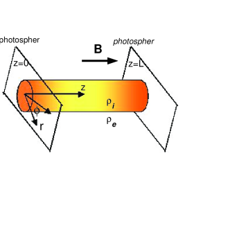
Figure 1: A sketch of the equilibrium model of the flux tube. Density varies along the cylinder axis and is symmetric about the midpoint. The magnetic field is uniform along the $z$-axis.

The linearized ideal MHD equations for the Eulerian perturbation in the velocity and the magnetic fields in a zero-$\beta$ plasma are

$$\frac{\partial\delta\mathbf{v}}{\partial t}=\frac{1}{4\pi\rho}\{(\mathbf{\nabla}\times\delta\mathbf{B})\times\mathbf{B}+(\mathbf{\nabla}\times\mathbf{B})\times\delta\mathbf{B}\},$$ (6)

$$\frac{\partial\delta\mathbf{B}}{\partial t}=\mathbf{\nabla}\times(\delta\mathbf{v}\times\mathbf{B}).$$ (7)

Note that Eq. (7) ensures the Gaussian law, $\nabla.\leavevmode\nobreak\ \delta\mathbf{B}=0$. From Eqs. (6) and (7) one can show, after some straightforward calculations that

$$\!\!\!\!\left(\frac{\omega^{2}}{v_{A}^{2}}+\frac{\partial^{2}}{\partial z^{2}}-\frac{m^{2}}{r^{2}}\right)\frac{\delta B_{z}}{B}=\left(\frac{\omega^{2}}{v_{A}^{2}}+\frac{\partial^{2}}{\partial z^{2}}\right)\frac{1}{r}\frac{\partial}{\partial r}\left(r\frac{\delta v_{r}}{i\omega}\right),$$ (8)

$$\!\!\!\!\left(\frac{\omega^{2}}{v_{A}^{2}}+\frac{\partial^{2}}{\partial z^{2}}\right)\frac{\delta v_{r}}{i\omega}=-\frac{\partial}{\partial r}\frac{\delta B_{z}}{B},$$ (9)

where $v_{A}(z,\epsilon)=B/\sqrt{4\pi\rho(z,\epsilon)}$ is the local Alfvén speed and is different for inside and outside of the loop. The term $\delta v_{r}/i\omega$ appearing in Eqs. (9) and (8) is actually the Lagrangian displacement vector in the loop. The remaining components of $\delta\mathbf{v}$ and $\delta\mathbf{B}$ are given by

$$\delta v_{\phi} = \frac{\omega}{mB_{z}}r\delta B_{z}-\frac{1}{im}\frac{\partial}{\partial r}(r\delta v_{r}),\leavevmode\nobreak\ \leavevmode\nobreak\ \leavevmode\nobreak\ \delta v_{z}=0,$$ (10)

$$\delta B_{r} = -\frac{B_{z}}{i\omega}\frac{\partial\delta v_{r}}{\partial z},\leavevmode\nobreak\ \leavevmode\nobreak\ \leavevmode\nobreak\ \leavevmode\nobreak\ \delta B_{\phi}=-\frac{B_{z}}{i\omega}\frac{\partial\delta v_{\phi}}{\partial z}.$$ (11)

See, e. g., Karami et al (2002) and Safari et al. (2006) for details. Let us also emphasize that the present form of Eq. (9) utilizes the fact that $\rho$ and, consequently, $v_{A}$ depend only on $z$. There is no radial variation except for a step discontinuity at the surface of the tube.

Eliminating $\delta v_{r}$ between Eqs. (9) and 8) gives

$$\left(\frac{1}{r}\frac{\partial}{\partial r}r\frac{\partial}{\partial r}+\frac{\partial^{2}}{\partial z^{2}}-\frac{m^{2}}{r^{2}}\right)\delta B_{z}+\frac{\omega^{2}}{v_{A}^{2}}\delta B_{z}=0.$$ (12)

This is a wave equation for $\delta B_{z}$ with the variable speed $v_{A}(\epsilon,z)$. We solve it by the separation of variables. Let $\delta B_{z}=R(r)Z(z)$. For later convenience, we add and subtract the term $\frac{\omega^{2}}{v_{A}^{2}(\epsilon=0)}\delta B_{z}$ to and from Eq. (12), and follow the usual procedure for the separation of variables. We obtain

$$\!\!\!\!\frac{1}{R}\frac{1}{r}\frac{d^{2}R}{dr^{2}}+\frac{1}{R}\frac{dR}{dr}-\frac{m^{2}}{r^{2}}+\frac{\omega^{2}}{v_{A}^{2}(\epsilon=0)}$$

$$\!\!\!\!\leavevmode\nobreak\ \leavevmode\nobreak\ =-\frac{1}{Z}\frac{d^{2}Z}{dz^{2}}-\omega^{2}\left(\frac{1}{v_{A}^{2}(\epsilon,z)}-\frac{1}{v_{A}^{2}(\epsilon=0)}\right)=\kappa_{z}^{2},$$ (13)

where $\kappa_{z}^{2}(\epsilon)$ is the constant of separation; and in the absence of longitudinal stratification, it reduces to the longitudinal wave number. Equation (13) may now be written as

$$\!\!\!\!\left(\frac{d^{2}}{dr^{2}}+\frac{1}{r}\frac{d}{dr}-\frac{m^{2}}{r^{2}}\right)R(r)+k^{2}R(r)=0,$$ (14)

$$\!\!\!\!\left(\frac{d^{2}}{dz^{2}}-k^{2}\right)Z(z)+\frac{\omega^{2}}{v_{A}^{2}}Z(z)=0,\leavevmode\nobreak\ \leavevmode\nobreak\ k^{2}=\frac{\omega^{2}}{v_{A}^{2}|_{\epsilon=0}}-\kappa_{z}^{2}.$$ (15)

Both Eqs. (14) and (15) are actually a pair for inside, $r<a$, and outside, $r>a$, of the tube. They are to be solved simultaneously for $R$, $Z$, $\kappa_{z}$, and $\omega$.

2.1 Boundary conditions

1. The changes in total pressure should be continuous. On account of the zero-$\beta$ approximation and constancy of $B$, this reduces to the requirement of the continuity of $\delta B_{z}$. Thus

   $$\!\!\!\!R^{\rm{interior}}(a)=R^{\rm{exterior}}(a),$$ (16)

   $$\!\!\!\!Z^{\rm{interior}}=Z^{\rm{exterior}},\leavevmode\nobreak\ \leavevmode\nobreak\ \leavevmode\nobreak\ \leavevmode\nobreak\ {\rm for\leavevmode\nobreak\ all\leavevmode\nobreak\ }z.$$ (17)

2. On account of $\mathbf{\nabla}\cdot\delta\mathbf{B}=0$, $\delta B_{r}$ should be continuous at $r=a$. This, gives (Karami et al 2002)

   $$\left.\frac{1}{k_{i}^{2}}\frac{dR^{\rm{interior}}(k_{i}r)}{dr}\right|_{r=a}=-\left.\frac{1}{k_{e}^{2}}\frac{dR^{\rm{exterior}}(k_{e}r)}{dr}\right|_{r=a}.$$ (18)

3. The footpoints, $z=0\leavevmode\nobreak\ \&\leavevmode\nobreak\ L$, are expected to be nodes. This imposes the conditions

   $$Z(z=0\leavevmode\nobreak\ \&\leavevmode\nobreak\ L)=0.$$ (19)

   Equations (16), (18), and (19) give four boundary conditions for the two second-order differential Eqs. (14) & (15).

3 Solutions of Eqs. (14) and (15)

Interior solutions of Eq. (14) that are regular at $r=0$ are $J_{m}(|k_{i}|r)$ for $k_{i}^{2}>0$ or $I_{m}(|k_{i}|r)$ for $k_{i}^{2}<0$. Exterior solutions that decay with $r\to\infty$ are $K_{m}(|k_{e}|r)$. They occur for $k_{e}^{2}<0$ and are evanescent waves.

Imposing the boundary conditions of Eqs. (16) and (18) gives

$$\frac{1}{k_{i}}\frac{J_{m}^{\prime}(|k_{i}|a)}{J_{m}(|k_{i}|a)}-\frac{1}{k_{e}}\frac{K_{m}^{\prime}(|k_{e}|a)}{K_{m}(|k_{e}|a)}=0,$$ (20)

where ^′ indicates a derivative of a function with respect to its argument. The same relation holds for surface waves with $J_{m}(|k_{i}|r)$ replaced by $I_{m}(|k_{i}|r)$. For unstratified thin and thick tubes Eq. (20) is analyzed by Edwin & Roberts (1983). Here we study Eq. (20) for thin stratified loops by perturbational and numerical techniques.

4 Thin tube approximation

For $a/L\ll 1$ and $m\geq 1$, the dispersion relation of Eq. (20) gives $|k_{i}|\approx|k_{e}|$. From the definition of $k^{2}$ in Eq. (14), one then obtains

$$\omega=\kappa_{z}B(4\pi\bar{\rho}_{0})^{-1/2},\leavevmode\nobreak\ \bar{\rho}_{0}=\frac{1}{2}[\rho_{i}(0)+\rho_{e}(0)].$$ (21)

This is the kink oscillation frequency in the presence of stratification. Edwin & Roberts (1978), Karami et al. (2002), Van Doorsselaere et al. (2004), and Díaz et al. (2004) all obtained a similar result for $\omega$ in unstratified flux tubes. Here, however, $\kappa_{z}$ is given by Eq. (13). It reduces to the longitudinal wave number in the absence of stratification. Substituting Eq. (21) into Eq.(15) (interior with $k_{i}^{2}>0$ and exterior with $k_{e}^{2}<0$) and using the boundary condition of Eq. (17) yield

$$\!\!\!\!\frac{d^{2}Z}{dz^{2}}+\frac{4\pi\omega^{2}}{B^{2}}F(\epsilon,z)Z(z)=0,\leavevmode\nobreak\ \leavevmode\nobreak\ Z=Z^{\rm interior}=Z^{exterior},$$ (22)

$$\!\!\!\!F(\epsilon,z)=\frac{\rho_{i}(\epsilon)+\rho_{e}(\epsilon)}{2}f(\epsilon,z).$$

Equation (22) is an eigenvalue problem weighted by $F(\epsilon,z)$. It is the same as that of Dymova & Ruderman (2005) derived, however, with a different approach.

From Eq. (22) one may write down the following integral expression for $\omega^{2}$

$$\omega^{2}=\frac{B^{2}}{4\pi}\frac{\int|dZ/dz|^{2}dz}{\int F(\epsilon,z)|Z(z)|^{2}dz}.$$ (23)

Some general properties of $\omega^{2}$ can be inferred from Eq. (23). In Fig. 3, $F(\epsilon,z)$ is plotted versus $z$ for three values of $\epsilon$. It has maxima at footpoints and a minimum at the apex. The larger $\epsilon$, the higher the maxima and the lower apex become. This reduces the integral in the denominator of Eq. (23) and causes an increase in $\omega^{2}$. There is even the possibility of the integral, and thereby $\omega^{2}$, becoming infinity.

In the following section, Eq. (22) is solved for small amount of the density scale heights by perturbation, and for arbitrary scale height parameters numerically.

4.1 Perturbation method

The scale height parameter is chosen as the perturbation parameter, and all variables and equations are expanded in powers of $\epsilon$. Thus,

$$\!\!\!\!\omega=\omega^{(0)}+\epsilon\omega^{(1)}+\cdots,$$ (24)

$$\!\!\!\!Z(z)=Z^{(0)}(z)+\epsilon Z^{(1)}(z)+\cdots,$$ (25)

$$\!\!\!\!F(\epsilon,z)=\bar{\rho}_{0}\left[1+\epsilon\left(\frac{2}{\pi^{2}}-\frac{1}{\pi}\sin\pi\frac{z}{L}\right)+\cdots\right].$$ (26)

Equation (22) splits into zeroth and first-order components

$$\!\!\!\!\frac{d^{2}Z^{(0)}}{dz^{2}}+\frac{4\pi\omega^{(0)^{2}}\bar{\rho}_{0}}{B^{2}}Z^{(0)}=0,$$ (27)

$$\!\!\!\!\frac{d^{2}Z^{(1)}}{dz^{2}}+\frac{4\pi\omega^{(0)^{2}}\bar{\rho}_{0}}{B^{2}}Z^{(1)}+\frac{8\pi\omega^{(0)}\omega^{(1)}\bar{\rho}_{0}}{B^{2}}Z^{(0)}$$

$$\!\!\!\!=-\frac{4\pi\omega^{(0)^{2}}\bar{\rho}_{0}}{B^{2}}\left(\frac{2}{\pi^{2}}-\frac{1}{\pi}\sin\frac{\pi z}{L}\right)Z^{(0)}.$$

(28)

Solutions of Eq. (27) for $Z^{(0)}$ and $\omega^{(0)}$ with boundary conditions of Eq. (19) are

$$\!\!\!\!\omega^{(0)}_{l}=\frac{l\pi}{L}B\leavevmode\nobreak\ (4\pi\bar{\rho}_{0})^{-1/2}\leavevmode\nobreak\ \leavevmode\nobreak\ l=1,2,3,...,$$ (29)

$$\!\!\!\!Z_{l}^{(0)}(z)=\sqrt{\frac{2}{L}}\sin\frac{l\pi}{L}z,$$ (30)

where $l$ is the longitudinal mode number, and $\omega^{(0)}_{l}$ the kink mode frequency in the absence of stratification. The right hand side of Eq. (28) is now known. Multiplying it by $Z^{(0)*}$, integrating over $z$, and reducing it by Eq. (27) gives the first-order corrections

$$\!\!\!\!{\omega}^{(1)}_{l}=\omega^{(0)}_{l}\frac{1}{2}(I_{ll}-\frac{2}{\pi^{2}})$$ (31)

$$\!\!\!\!Z_{l}^{(1)}=\sum_{l^{\prime}\neq l}c_{ll^{\prime}}Z^{(0)}_{l^{\prime}},\leavevmode\nobreak\ \leavevmode\nobreak\ c_{ll^{\prime}}=\frac{l^{2}I_{ll^{\prime}}}{l^{2}-l^{\prime 2}},$$ (32)

where

$$I_{ll^{\prime}} = \int_{0}^{L}Z^{(0)*}_{l^{\prime}}\frac{1}{\pi}sin\frac{\pi z}{L}Z^{(0)}_{l}dz$$ (33)

$$= -\frac{4}{\pi^{2}}\frac{ll^{\prime}(1+\cos l\pi\cos l^{\prime}\pi)}{l^{4}+(-1+l^{\prime 2})^{2}-2l^{2}(1+l^{\prime 2})}.$$

Equation (33) agrees with the result of Andries et al. (2005a) ( see $S_{n}$ in their Eqs. (3) and (4)). The Sheffield school maintains that a knowledge of the deviations of the amplitude profile of stratified loops from those of the unstratified one, $Z_{l}-Z_{l}^{(0)}\approx\epsilon Z_{l}^{(1)}$, in our notation can give information on the density stratification of the loop (private communication, see also Erdélyi & Verth 2007). In Fig. 2, $Z^{(1)}_{1}$ and $Z^{(1)}_{2}$ are plotted as functions of $z$. The first, $Z^{(1)}_{1}$, exhibits two maxima at $z/L=1/6\leavevmode\nobreak\ \&\leavevmode\nobreak\ 5/6$ and one minimum at $1/2$. It is zero at $0,\leavevmode\nobreak\ 1/3,\leavevmode\nobreak\ 2/3,\leavevmode\nobreak\$ and $1$. The second, $Z^{(1)}_{2}$, shows two maxima at $z/L=1/8\leavevmode\nobreak\$ and $5/8$, two minima at $3/8$ and $7/8$, and is zero at $0,\leavevmode\nobreak\ 1/4,\leavevmode\nobreak\ 2/4,\leavevmode\nobreak\ 3/4,$ and $1$. The maxima of $Z_{1}^{(1)}/Z_{1}^{(0)}$ and $Z_{2}^{(1)}/Z_{2}^{(0)}$ are 0.02 and 0.04, respectively; see Table 1 column 2 & 4. From the TRACE data, Aschwanden et al. (2002) report a displacement amplitude of 100-8800 km at the apex of the coronal loops. For a loop of $L=$100 Mm, $\epsilon=L/H=2$, the calculated percentages, 0.02-0.04, ${\rm{Max}}(\Delta Z_{1})$ fall in the range 2-176 km. One should be aware of whether the accuracies of observed data allows the detection of such minute effects.

We note that $\omega^{(1)}$ is positive and tends to zero for $l\gg 1$. The ratio of the periods of the fundamental and the first overtone is

$$\frac{P_{1}}{P_{2}} = \frac{\omega_{2}}{\omega_{1}}$$ (34)

$$= 2\frac{1+\epsilon\omega_{2}^{(1)}/\omega_{2}^{(0)}}{1+\epsilon\omega_{1}^{(1)}/\omega_{1}^{(0)}}=2\frac{1+\epsilon\frac{1}{15\pi^{2}}}{1+\epsilon\frac{1}{3\pi^{2}}}<2.$$

Equation (34) is a useful tool to estimate the density scale height of the loops, see also Roberts (2005).

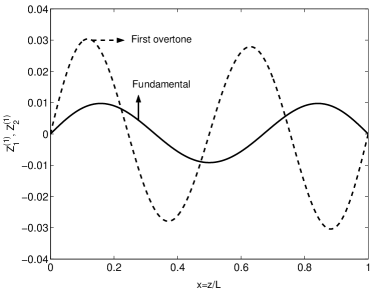
Figure 2: Plot of the first-order perturbations in amplitude profiles of the fundamental and the first overtone modes. See Eqs. (30) and (32).

4.2 Numerical method

Using a numerical code based on shooting method, Eq. (22) is solved for eigenvalues and eigenfunctions. For the unstratified loops, where $\rho_{i}$ and $\rho_{e}$ are constants, the eigenfrequencies and the eigenfunctions are those of Eqs. (29) and (30), respectively. For a range of $0<\epsilon/\pi<25$, we have calculated the fundamental and the first overtone kink frequencies $\omega_{1}$ and $\omega_{2}$, respectively, and the ratio $\omega_{2}/\omega_{1}=P_{1}/P_{2}$. The results are plotted in Fig. 4. As anticipated from Eq. (23) and the behavior of $F(\epsilon,z)$, both frequencies show monotonous increase with increasing $\epsilon$. For small $\epsilon$, $\omega_{1}$ has a steeper slope than $\omega_{2}$, but both approach each other as $\epsilon$ increases. The ratio $P_{1}/P_{2}$ begins at 2 for unstratified loops, $\epsilon=0$, and decreases to one at large $\epsilon$. From the TRACE data, Verwichte et al. (2004) find the ratio 1.64 and 1.81 for two of their observed loops. From Fig. 4, $\epsilon$ corresponding to these ratio are 1.93$\pi$ and 1.07$\pi$, respectively. Assuming typical loop lengths, $L=100-250$ Mm, the density scale height falls in the range of $H\approx$16-41 and 30-74 Mm, respectively. These scale heights agree with the finding of Andries et al. (2005a, b).

The longitudinal part of the eigenfield, $Z(z)$, is plotted in Figs. 5 for $l=$1, 2, 3 and $\epsilon=$0, 2, 5. As $\epsilon$ increases, a) the eigenprofiles depart further from the sinusoidal profiles of the unstratified case, b) the antinodes move towards the footpoints, and c) the central antinode gets flattened in the case of odd $l$.

The differences between the eigenprofiles of the stratified and the unstratified cases, $\Delta Z_{l}=Z_{l}(\epsilon,z)-Z_{l}(\epsilon=0,z)$, are plotted in Fig. 6 for the fundamental and the first overtone modes. Expectedly, the difference increases with increasing $\epsilon$. The maxima rise and move towards the footpoints as $\epsilon$ increases. For example, for $\epsilon=2$ and $5$ ( corresponding to $L=200$Mm, $H=50$ and $20$Mm, say ), the first maximum of $\Delta Z_{1}$ is located at $z=$36Mm and 35Mm, respectively, in agreement with Erdélyi & Verth (2007).

Table 1 shows ${\rm Max}(\Delta Z_{l}/\epsilon Z_{l})$ for $l=$1, 2 and $\epsilon=2$, 5. Columns 2 and 4 are from the first order perturbation calculations. Column 3 and 5 are from the full numerical analysis. The proximity of the two different methods of calculations, even at scale heights as large as $\epsilon=5$, is striking.

Table 1: Maximum amplitude differences between stratified and unstratified loops, 1st-order perturbation ( columns 2 & 4 ), and full numerical calculations ( columns 3 & 5 ).

$\epsilon=\frac{L}{H}$	${\rm Max}\left(\frac{\Delta Z_{1}}{\epsilon Z^{(0)}_{1}}\right)$	${\rm Max}\left(\frac{\Delta Z_{2}}{\epsilon Z^{(0)}_{2}}\right)$
	Perturbation   Numerical	Perturbation   Numerical
2	0.02             0.017	0.04             0.036
5	0.02            0.022	0.04              0.04

Aschwanden et al. (2002) report a displacement amplitude of 100-8800 km at the apex of the kink modes. Combined with the fractional deviations of Table 1, one may calculate actual physical deviations of 2-176 km for $\epsilon=2$ and $6-528$km for $\epsilon=5$. This result also agrees with Erdélyi & Verth (2007). The question remains as to whether the accuracy of the observed data will allow the detection of such small effects.

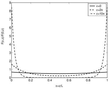
Figure 3: $F(\epsilon,z)$ versus $z/L$. $\epsilon=0.0$ (solid line), $\epsilon=2\pi$ (dashed line), and $\epsilon=10\pi$ (dot dashed line) . As $\epsilon$ increases, $F(\epsilon,z)$ recedes towards the end points and is void around where the mid point widens.

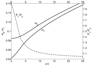
Figure 4: The frequencies, $\omega_{1}$ and $\omega_{2}$, and the ratio $P_{1}/P_{2}=\omega_{2}/\omega_{1}$ versus $\epsilon/\pi$. Auxiliary parameters are the tube length =$100a$, B = 100 G, and $\rho_{e}/\rho_{i}=0.1$.

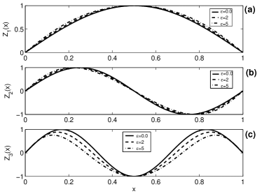
Figure 5: a) The fundamental mode ($l=1$), b) the first overtone mode ($l=2$), and c) the second overtone modes ($l=3$) versus z, for unstratified, $\epsilon=0$, ( corresponding to $H=\infty$, $L$=100Mm , say ) and stratified, $\epsilon=2,\leavevmode\nobreak\ 5$, ( corresponding to $H=50$ & 20Mm and $L=100$Mm, say ).

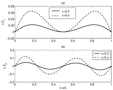
Figure 6: Amplitude differences of the fundamental and first overtone modes from those of the unstratified loops for $\epsilon=2$ & 5, numerical calculations.

5 CONCLUSIONS

We have studied the MHD oscillations of a vertically stratified coronal loop

• Equation (22), for the longitudinal component of the waves, is the same as those of Dymova & Ruderman (2005).

• The oscillations frequencies, obtained from Eq. (22), depend on the stratification parameter $\epsilon$. This in turn, makes the radial wave numbers, $k_{i}$ & $k_{e}$ of Eqs. (15) and (20) $\epsilon$- dependent.

• In the thin tube approximation, the eigenfrequencies are obtained by both perturbational and numerical techniques.

• The effect of stratification is best understood by the behavior of $F(\epsilon,z)$, highlighted in Fig. 3. $F(\epsilon,z)$ is all positive. But at large $\epsilon$ it becomes insignificant in broad neighborhood of $z=L/2$. This reduces the denominator in Eq. (23) and lets $\omega^{2}$ grow. This in turn results in washing-out finite time measurements of the phenomena under study.

• The ratio of the periods of the fundamental and the first overtone modes (2 for unstratified loops) decreases markedly and approaches 1 with an increasing density-scale height parameter. For $\rho_{e}/\rho_{i}=0.1$, $\epsilon/\pi=L/\pi H=1.07$, & $1.94$, the ratio $P_{1}/P_{2}$ is $1.81$ & $1.64$. These are in good agreement with the observational data of Verwichte et al. (2004), $1.81\pm 0.25$ and $1.64\pm 0.23$. The latter are deductions from TRACE observations, assuming the same density contrast and scale height parameter.

• The eigenfunctions of stratified loops deviate from the sinusoidal profiles of the unstratified ones. Relative deviations grow with $\epsilon$ and are of are close to a few percent, in general (see Table 1).

- (1) Andries, J., Goossens, M., Hollweg, J. V., Arregui, I., & Van Doorsselaere, T. 2005a, A&A, 430, 1109
- (2) Andries, J., Arregui, I., & Goossens, M. 2005b, ApJ, 24L, 57
- (3) Aschwanden, M. J. 2003, Coronal MHD Waves and Oscillations: Observations and Quests; in Erdélyi et al. (eds) Turbulence, Waves and Instabilities in the Solar Plasma, NATO Science Series, II. Mathematics, Physics and Chemistry, Vol. 124, Kluwer, pp.1-31
- (4) Aschwanden, M. J., De Pontieu, B., Schrijver, C. J., & Title, A. M. 2002, Sol. Phys., 206, 99
- (5) Aschwanden, M. J., Fletcher, L., Schrijver, C. J., & Alexander, D. 1999a, ApJ, 520, 880
- (6) Aschwanden, M. J., Newmark, J. S., Delaboudiniére, J., Neupert, W. M., Klimchuk, J. A., et al. 1999b, ApJ, 515, 842
- (7) Bennett, K., Roberts, B., & Narain, U. 1998, Sol. Phys., 185, 41
- (8) De Pontieu, B., Erdélyi, & R., de Wijn, A. G. 2003a, ApJ, 595, L63
- (9) De Pontieu, B., Tarbell, T. & Erdélyi, R. 2003b, ApJ, 590, 502
- (10) Díaz, A. J., Oliver, R., Ballester, J. L., & Roberts, B. 2004, A&A, 424, 1055
- (11) Díaz, A. J., Oliver, R., Erdélyi, R., & Ballester, J. L. 2001, A&A, 379, 1083
- (12) Dymova, M.V., & Ruderman, M.S. 2005, Sol. Phys., 229, 79
- (13) Edwin, P. M., & Roberts, B. 1983, Sol. Phys., 88, 179
- (14) Erdélyi, R., & Carter, B. K. 2006, A&A, 455, 361
- (15) Erdélyi, R., & Fedun, V. 2006, Sol. Phys, 238, 41
- (16) Erdélyi, R., & Verth, G. 2007, A&A, 462, 743
- (17) Gradshteyn, I. S., & Ryzbik, I. M. 2000, Academic Press, Table of Integrals, Series, and Products, Edition, 933
- (18) Karami, K., Nasiri, S. & Sobouti, Y. 2002, A&A, 396, 993
- (19) Mendoza-Briceño, César A., Erdélyi, R., & Sigalotti, Leonardo Di G. 2004, ApJ, 605, 493
- (20) Mikhalyaev, B. B., & Solovév, A. A. 2005, Sol. Phys, 227, 249
- (21) Nakariakov, V. M., Ofman, L., Deluca, E. E., Roberts, B., & Davila, J. M. 1999, Science, 285, 862
- (22) Nakariakov, V. M., & Verwichte, E. 2005, LRSP, 2, 3
- (23) Nasiri, S. 1992, A&A, 261, 615
- (24) Roberts, B. 2005, Phil. Trans. R. Soc. A, 364, 447
- (25) Ruderman, M. S. 2003, A&A 409, 287
- (26) Safari, H., Nasiri, S., Karami, K., & Sobouti, Y. 2006, A&A, 448, 375.
- (27) Schrijver, C. J., Aschwanden, M. J., & Title, A. 2002, Sol. Phys., 206, 69
- (28) Smith, J. M., Roberts, B., & Oliver, R. 1997, A&A, 317, 752
- (29) Terra-Homem, M., Erdélyi, R.,& Ballai, I. 2003, Sol. Phys., 217, 199
- Van Doorsselaere et al. (2004) Van Doorsselaere, T., Debosscher, A., Andries, J., & Poedts, S. 2004, A&A, 424, 1065
- (31) Verwichte, E., Nakariakov, V.M., Ofman, L., & DeLuca, E. E. 2004, Sol. Phys., 223, 77
- (32) Wang, T. J., & Solanki, S. K. 2004, A&A, 421, L33