Escape fraction of ionizing photons from galaxies at $z=0$–$6$

Abstract

The escape fraction of ionizing photons from galaxies is a crucial quantity controlling the cosmic ionizing background radiation and the reionization. Various estimates of this parameter can be obtained in the redshift range, $z=0$–6, either from direct observations or from the observed ionizing background intensities. We compare them homogeneously in terms of the observed flux density ratio of ionizing ($\sim 900$ Å rest-frame) to non-ionizing ultraviolet ($\sim 1500$ Å rest-frame) corrected for the intergalactic absorption. The escape fraction is found to increase by an order of magnitude, from a value less than 0.01 at $z\la 1$ to about $0.1$ at $z\ga 4$.

1 Introduction

Although recent observations have revealed the outline of the cosmic reionization (Page et al., 2006; Fan et al., 2006), its detailed history and the nature of ionizing sources are not yet fully understood. Early forming galaxies can be strong ionizing sources, depending on the escape fraction of their ionizing photons ($f_{\rm esc}$). This $f_{\rm esc}$ is therefore a key quantity for understanding the cosmic reionization process but its typical (or effective) value is not yet clearly established (e.g., Inoue et al., 2005).

The goal of this Letter is to put together all existing information on the amount of ionizing photons released by galaxies into the intergalactic medium (IGM), both from direct observations and from indirect estimations based on the effects of the IGM ionization itself. In order to make an homogeneous comparison, we introduce a quantity derived from $f_{\rm esc}$, the escape flux density (Hz^-1) ratio of the Lyman continuum (LyC, $\lambda\sim 900$ Å  rest-frame) to the non-ionizing ultraviolet (UV, $\lambda\sim 1500$ Å  rest-frame), ${\cal R}_{\rm esc}$. This ${\cal R}_{\rm esc}$ is naturally measured by direct observations (e.g., Steidel et al., 2001). We compile all the observations of the LyC from galaxies and derive ${\cal R}_{\rm esc}$ at $z\la 3$. On the other hand, ${\cal R}_{\rm esc}$ can be derived from the ionizing background intensity inferred from IGM absorption measurements via a cosmological radiative transfer model. We derive ${\cal R}_{\rm esc}$ at $z=0$–6 based on the recent reports of the background intensities.

The cosmological parameters assumed in this Letter are $H_{0}=70.0$ km s^-1 Mpc^-1, $\Omega_{\rm m}=0.3$, and $\Omega_{\Lambda}=0.7$.

2 Formulation

The definition of $f_{\rm esc}$ in this Letter is

$$f_{\rm esc}=\frac{F_{\rm LyC}^{\rm esc}}{F_{\rm LyC}^{\rm int}}\,,$$ (1)

where $F_{\rm LyC}^{\rm int}$ and $F_{\rm LyC}^{\rm esc}$ are the intrinsic and escaping LyC flux densities, respectively. To obtain $F_{\rm LyC}^{\rm esc}$, we have to correct the observed LyC flux density $F_{\rm LyC}^{\rm obs}$ for the photoelectric absorption by the neutral hydrogen remained in the IGM:

$$F_{\rm LyC}^{\rm esc}=F_{\rm LyC}^{\rm obs}e^{\tau_{\rm LyC}^{\rm IGM}}\,.$$ (2)

We may estimate $F_{\rm LyC}^{\rm int}$ from the observed UV flux density $F_{\rm UV}^{\rm obs}$ as follows:

$$F_{\rm LyC}^{\rm int}={\cal R}_{\rm int}F_{\rm UV}^{\rm obs}e^{\tau_{\rm UV}^{\rm ISM}}\,,$$ (3)

where ${\cal R}_{\rm int}=F_{\rm LyC}^{\rm int}/F_{\rm UV}^{\rm int}$ is the intrinsic LyC-to-UV flux density ratio and $\tau_{\rm UV}^{\rm ISM}$ is the UV dust opacity in the interstellar medium of a galaxy. Therefore, we have

$$f_{\rm esc}=\frac{{\cal R}_{\rm esc}}{{\cal R}_{\rm int}}e^{-\tau_{\rm UV}^{\rm ISM}}\,,$$ (4)

and

$${\cal R}_{\rm esc}=\frac{F_{\rm LyC}^{\rm obs}}{F_{\rm UV}^{\rm obs}}e^{\tau_{\rm LyC}^{\rm IGM}}\,.$$ (5)

This ${\cal R}_{\rm esc}$ is called the LyC-to-UV escape flux density ratio in this Letter. As found in equation (5), we can obtain ${\cal R}_{\rm esc}$ from the observed LyC-to-UV flux density ratio with a correction for the IGM absorption against the LyC. This is similar to the approach introduced by Steidel et al. (2001).

On the other hand, ${\cal R}_{\rm esc}$ can be obtained from the observed ionizing background intensity through a cosmological radiative transfer model. We describe the different aspects of this estimation in the four following sub-sections.

2.1 Cosmological Lyman continuum transfer

The mean specific intensity at the observed frequency $\nu_{\rm o}$ as seen by an observer at redshift $z_{\rm o}$ is given by (e.g., Peebles, 1993)

$$J(\nu_{\rm o},z_{\rm o})=\frac{(1+z_{\rm o})^{3}}{4\pi}\int_{z_{\rm o}}^{z_{\rm i}}dz\frac{dl}{dz}(z)\rho(\nu,z)e^{-\tau_{\rm eff}(\nu_{\rm o},z_{\rm o},z)}\,,$$ (6)

where the frequency $\nu=\nu_{\rm o}(1+z)/(1+z_{\rm o})$, $dl/dz$ is the line element, $\rho$ is the emissivity per unit comoving volume, and $\tau_{\rm eff}$ is the effective IGM opacity. Although the upper limit of the integral could be infinity, we set it to $z_{\rm i}$. The line element is

$$\frac{dl}{dz}(z)=\frac{c}{H(z)(1+z)}\,,$$ (7)

where $c$ is the speed of light and $H$ is the Hubble parameter. The comoving emissivity can be written as

$$\rho(\nu,z)=\rho_{\rm QSO}(\nu,z)+\rho_{\rm gal}(\nu,z)\,,$$ (8)

where $\rho_{\rm QSO}$ and $\rho_{\rm gal}$ are the QSO and galactic emissivities, respectively. The IGM emissivity can be omitted (see §2.3). The effective IGM opacity is (e.g., Paresce et al., 1980)

$$\tau_{\rm eff}(\nu_{\rm o},z_{\rm o},z)=\int_{z_{\rm o}}^{z}dz^{\prime}\int_{N_{\rm l}}^{N_{\rm u}}dN_{\rm HI}\frac{\partial^{2}{\cal N}}{\partial N_{\rm HI}\partial z}(1-e^{-\tau})\,,$$ (9)

where $\partial^{2}{\cal N}/\partial N_{\rm HI}\partial z$ is the cloud number on a line of sight per unit redshift $z$ interval and per unit H i column density $N_{\rm HI}$ interval, and $N_{\rm l}$ and $N_{\rm u}$ are the lower and upper limits of the column density of the IGM clouds. The cloud optical depth is $\tau=\sigma_{\rm H}(\nu^{\prime})N_{\rm HI}$ with $\sigma_{\rm H}$ the hydrogen cross-section at the frequency $\nu^{\prime}=\nu_{\rm o}(1+z^{\prime})/(1+z_{\rm o})$. The frequency dependence of $\sigma_{\rm H}$ for the LyC is assumed to be $\propto\nu^{-3}$.

2.2 IGM opacity

The effective IGM opacity is determined by the cloud number function which can be expressed as (e.g., Miralda-Escudé & Ostriker, 1990)

$$\frac{\partial^{2}{\cal N}}{\partial N_{\rm HI}\partial z}\propto{N_{\rm HI}}^{-\beta}(1+z)^{\gamma}\,.$$ (10)

If we assume a single index $\beta$ $(1<\beta<2)$ for all $N_{\rm HI}$ and $z$, and $N_{\rm l}\sigma_{\rm H}\ll 1$ and $N_{\rm u}\sigma_{\rm H}\gg 1$, equation (9) can be approximated to (Zuo & Phinney, 1993; Inoue et al., 2005)

$$\tau_{\rm eff}(\nu_{\rm o},z_{\rm o},z)\approx\int_{z_{\rm o}}^{z}\Gamma(2-\beta){\cal A}[N_{\rm l}\sigma_{\rm H}(\nu^{\prime})]^{\beta-1}(1+z^{\prime})^{\gamma}dz^{\prime}\,,$$ (11)

where $\Gamma$ is the usual Gamma function, $\cal A$ is the number of the IGM clouds with the column density between $N_{\rm l}$ and $N_{\rm u}$ on a line of sight per unit redshift interval, and $\nu^{\prime}=\nu_{\rm o}(1+z^{\prime})/(1+z_{\rm o})$. According to Weymann et al. (1998) and Kim et al. (2002), we assume $\beta=1.5$, $({\cal A},\gamma)=(34.5,0.2)$ for $z\leq 1.1$ and $({\cal A},\gamma)=(6.3,2.5)$ for $z>1.1$, and $N_{\rm l}=4.4\times 10^{13}$ cm^-2. Note that we have assumed the same number evolution along the redshift (the index $\gamma$) for the Ly$\alpha$ forest and for the Lyman limit system (and also for the damped Ly$\alpha$ clouds), whereas Madau (1995) adopted different indices for these clouds. As shown in the appendix of Inoue et al. (2005), the same $\gamma$ for all clouds is compatible with the recent observations of the Lyman limit systems by Péroux et al. (2003).

While the IGM opacity model is used in this paper for the LyC, we display in Fig. 1 the opacity predictions at Ly$\alpha$ line where comparisons with observations are possible. The Ly$\alpha$ cross-section is based on Wiese et al. (1966). Note that the same IGM clouds contribute to the LyC and Ly$\alpha$ opacities. Our model (solid line) shows a very good agreement with the data at $z<5$ but a smaller opacity than the data at $z>5$. An explanation is that the parameters of the cloud distribution taken from Kim et al. (2002) who analysed the Ly$\alpha$ forest at $z<4$. If we assume $({\cal A},\gamma)=(1.3,3.5)$ for $z>4$, the model (dashed line) shows a very good agreement with the data.

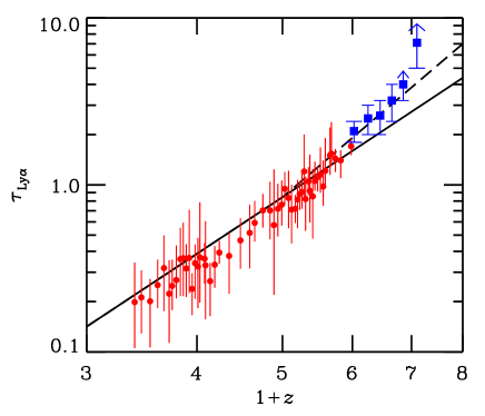
Figure 1: IGM Ly$\alpha$ opacity. The solid and dashed lines are the IGM Ly$\alpha$ opacities calculated by equation (11) (see the text for the detail). The circles and squares with error-bars are the observed opacity taken from Songaila (2004) and Fan et al. (2006), respectively.

2.3 Emissivities

The LyC emissivity from galaxies can be expressed as

$$\rho_{\rm gal}(\nu,z)=f(\nu){\cal R}_{\rm esc}(z)\rho_{\rm UV}^{\rm obs}(z)\,,$$ (12)

where $\rho_{\rm UV}^{\rm obs}$ is the observed galactic UV emissivity per unit comoving volume, and $f(\nu)$ is the LyC frequency dependence of galaxies. We assume that $f(\nu)\propto\nu^{-2}$ (e.g., Fioc & Rocca-Volmerange, 1997), independently of the redshift. The effect of the spectral slope on the estimated ${\cal R}_{\rm esc}$ is 15% at most if the index is changed from 0 to $-4$. A redshift dependence of ${\cal R}_{\rm esc}$ is introduced.

A key feature of equation (12) is that the LyC emissivity is directly related to the observed UV emissivity with the only parameter ${\cal R}_{\rm esc}$ that we wish to determine. In other words, our estimate for $R_{\rm esc}$ is free from uncertain dust correction and from the intrinsic LyC production rate (or ${\cal R}_{\rm int}$) which depends on the initial mass function.

The $\rho_{\rm UV}^{\rm obs}$ values are obtained from the integration to zero luminosity of UV luminosity functions compiled from the literature. They are shown as a function of redshift in Fig. 2. The error-bars indicate observational 1-$\sigma$ errors. For practical purpose, we express $\rho_{\rm UV}^{\rm obs}$ as the following functional form, $\rho_{\rm UV}^{\rm obs}(z)=\rho_{\rm UV}^{*}g(z)$, with

$$g(z)=\cases{\left(\frac{1+z}{2.7}\right)^{2}&($0\leq z<1.7)$\cr 1&($1.7\leq z<3.0$)\cr\left(\frac{1+z}{4.0}\right)^{-3.5}&($3.0\leq z$)\cr}\,.$$ (13)

The normalization adopted is $\rho_{\rm UV}^{*}=2.7\times 10^{26}$ erg s^-1 Hz^-1 Mpc^-3 based on Sawicki & Thompson (2006). $\rho_{\rm UV}^{\rm obs}$ of equation (13) is displayed as the solid line in Fig. 2 and called the standard case. Because of the scatter at $z>3$, we consider another case, the high-emissivity case, with $g(z)=1$ for $z\geq 3$, displayed in Fig. 2 as the dotted line.

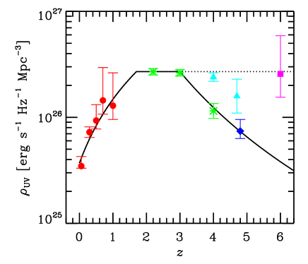
Figure 2: Observed total galactic UV emissivities per unit comoving volume. The circles, asterisks, diamonds, triangles, and squares are taken from Schiminovich et al. (2005), Sawicki & Thompson (2006), Iwata et al. (2006), Ouchi et al. (2004), and Bouwens et al. (2006), respectively. The solid and dotted lines are the standard and the high-emissivity cases assumed in the calculation, respectively.

The QSO emissivity is given by the prescription in Bianchi et al. (2001) who obtained the LyC emissivity of QSOs based on the optical luminosity functions of Boyle et al. (2000) and Fan et al. (2001) and an average QSO spectrum. We here adopt a QSO spectrum parameterized by Madau, Haardt, & Rees (1999).

The ionized IGM can contribute to a fraction of the LyC emissivity by the recombination process (Haardt & Madau, 1996). However, it is obviously secondary. Thus, we omit it. Miniati et al. (2004) suggested a significant contribution to the LyC by the thermal emission from hot gas shock-heated by the cosmological structure formation. In spite of its hard spectrum, however, the estimated hydrogen ionization rate is an order of magnitude smaller than that reported by Bolton et al. (2005) at $z=2$–4 and is less than one-third of that reported by Fan et al. (2006) at $z=5$–6. Thus, we also omit the thermal emission by the structure formation. The omission of the IGM emissivity leads to an overestimate of ${\cal R}_{\rm esc}$ that should be less than a factor of 2.

2.4 Estimation of the LyC-to-UV escape flux density ratio

If we enter the IGM opacity model described in §2.2 and the LyC emissivities described in §2.3 into equation (6), we can predict the background intensity at the Lyman limit as a function of ${\cal R}_{\rm esc}$. This latter quantity can be evaluated by a comparison between the predicted and observed intensities.

The observed intensities are obtained in the following ways. At $z<4$, Scott et al. (2002) presented intensities at the Lyman limit based on their observations of the QSO proximity effect. Bolton et al. (2005) and Fan et al. (2006) estimated hydrogen ionization rates ($\Gamma_{\rm HI}$) at $z=2$–4 and at $z=5$–6, respectively, based on the observed IGM Ly$\alpha$ opacity and a cosmological hydrodynamical simulation. The ionization rate $\Gamma_{\rm HI}$ is

$$\Gamma_{\rm HI}=\int_{\nu_{\rm L}}^{\infty}\frac{4\pi\sigma_{\rm H}(\nu)J({\nu})}{h\nu}d\nu=\frac{4\pi\sigma_{\rm L}J_{\rm L}}{h(\alpha+3)}\,,$$ (14)

where the subscript L means the quantity at the Lyman limit, $h$ is the Planck constant, and $\alpha$ is the power-law index when we assume a power-law background radiation ($J\propto\nu^{-\alpha}$). Assuming $\alpha=2$, we have $J_{\rm L}/10^{-21}\,\,{\rm erg\,\,s^{-1}\,\,cm^{-2}\,\,Hz^{-1}\,\,sr^{-1}}=\Gamma_{\rm HI}/2.39\times 10^{-12}\,\,{\rm s}^{-1}$ with $\sigma_{\rm L}=6.30\times 10^{-18}$ cm² (Osterbrock, 1989). The uncertainty on $J_{\rm L}$ resulting from the adopted $\alpha$ is a factor of $(\alpha+3)/5$. With this conversion we obtain $J_{\rm L}$ from the $\Gamma_{\rm HI}$ values of Bolton et al. (2005) and Fan et al. (2006). We should note here that Fan et al. (2006) determined their absolute $\Gamma_{\rm HI}$ values so as to fit those of McDonald & Miralda-Escudé (2001) which are somewhat smaller than those of Bolton et al. (2005).

${\cal R}_{\rm esc}$ is determined by a comparison of these observed intensities at the Lyman limit ($J_{\rm L}^{\rm obs}$) with the calculated theoretical intensities as

$$J_{\rm L}^{\rm obs}(z)=J_{\rm L}^{\rm QSO}(z)+J_{\rm L}^{\rm gal}(z,{\cal R}_{\rm esc})\,,$$ (15)

where $J_{\rm L}^{\rm QSO}$ and $J_{\rm L}^{\rm gal}$ are the Lyman limit intensities originating from QSOs and galaxies, respectively. This comparison is performed by a non-parametric way from high to low redshift. Calculating $J_{\rm L}^{\rm gal}$ (and then ${\cal R}_{\rm esc}$) at a redshift, we use the ${\cal R}_{\rm esc}$ values at redshifts larger than the redshift. For three different references of the observed intensities, we estimate ${\cal R}_{\rm esc}$ independently. The assumed initial redshifts in equation (6) are 5.0, 5.0, and 6.0 for the data from Scott et al. (2002), Bolton et al. (2005), and Fan et al. (2006), respectively. This choice does not affect the results if we take an enough high redshift because the IGM opacity is very large at high redshift. In addition, we note that we assumed the higher opacity case at $z>4$ (shown in Fig. 1 as dashed line) only for the data from Fan et al. (2006).

3 Results

The values of ${\cal R}_{\rm esc}$ obtained at different redshifts either from direct observations or from indirect estimations (§2.4) are displayed in Fig. 3.

Figure 3: Escape flux density ratio of the ionizing to the non-ionizing UV photons. The symbols and arrows with a label are measurements and upper limits from direct observations: I05 (Inoue et al. 2005), S01 (Steidel et al. 2001), G02 (Giallongo et al. 2002), M03 (Malkan et al. 2003), L95/H97 (Leitherer et al. 1995, Hurwitz et al. 1997), D01 (Deharveng et al. 2001), and B06 (Bergvall et al. 2006). The circles and large downward arrows are the estimated value and upper limits based on the ionizing background intensities reported by Scott et al. (2002). Only upper limits are obtained at lower redshifts because the intensities from QSOs are almost equal to or exceed the observed intensities (see also Fig. 4). The triangles and squares are the estimated values based on the ionization rates reported by Bolton et al. (2005) and Fan et al. (2006), respectively; the standard emissivity of galaxies is assumed for the filled symbols, and the high-emissivity case is assumed for the open symbols. The dashed line is a possible fit to the evolution of ${\cal R}_{\rm esc}$ that will be used in Fig. 4.

Their comparison reveals an evolution of ${\cal R}_{\rm esc}$, with ${\cal R}_{\rm esc}$ getting larger at higher redshifts. If we put confidence in the upper limit of Malkan et al. (2003) at $z\sim 1$, which is an average value of ${\cal R}_{\rm esc}$ for 11 star-forming galaxies and is less affected than a single measurement by the randomness of the LyC escape, we can obtain a possible evolution, for example, as

$${\cal R}_{\rm esc}\propto(1+z)^{5}\,,$$ (16)

from $z=1.5$ to $z=4.0$, which is shown as the dashed line in Fig. 3. Since the uncertainties are still very large, this rather strong evolution is just an example. However, we note that an evolution of ${\cal R}_{\rm esc}$ is also found even in the high-emissivity case (open symbols). Such an increasing ${\cal R}_{\rm esc}$ was suggested by Meiksin (2005) in his Fig. 1 although the redshift coverage is smaller than ours.

The measurement by Steidel et al. (2001) is somewhat larger than our estimations. This may be caused by their sample selection bias. Indeed, their sample galaxies are taken from the bluest quartile in the UV colour among Lyman break galaxies. At lower redshifts, we have only upper limits, except for the measurement by Bergvall et al. (2006), and a large dispersion. This is probably due to the small number of the observed galaxies. Indeed, only 7 galaxies have been observed to date (Leitherer et al., 1995; Deharveng et al., 2001; Bergvall et al., 2006). The galaxy observed by Bergvall et al. (2006) (Haro 11) may be an exceptional one in the local Universe as discussed in their paper.

Fig. 4 shows a comparison of the calculated ionizing intensity with the observed ones. Assuming the evolution of ${\cal R}_{\rm esc}$ shown in Fig. 3 as the dashed line, we obtain the dotted line for the galactic contribution and the solid line for the total intensity. The dashed line is the QSO contribution. The main contributor to the ionizing background radiation changes from galaxies to QSOs at $z\sim 3$.

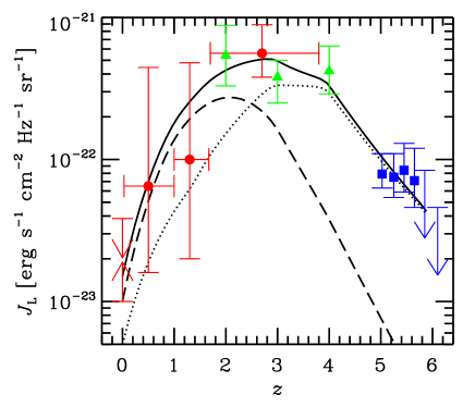
Figure 4: Lyman limit intensity of the background radiation. The circles and arrows at $z\simeq 0$ are measurements taken from Scott et al. (2002). The triangles and squares are converted from the ionization rates of Bolton et al. (2005) and Fan et al. (2006), respectively. The dashed line is the intensity from the QSOs (Bianchi et al. 2001). The solid and dotted lines are the total and galactic intensities, respectively. The standard galactic emissivity and an evolution of the escape flux density ratio shown in Fig. 3 as the dashed line are assumed.

4 Summary and discussion

We have discussed the escape flux density ratio of the LyC to the non-ionizing UV (${\cal R}_{\rm esc}$) in a new framework for comparing the direct observations of the LyC from galaxies with the cosmic ionizing background intensity. We have found a redshift evolution of ${\cal R}_{\rm esc}$, with larger ${\cal R}_{\rm esc}$ at higher redshifts. Here, we translate ${\cal R}_{\rm esc}$ into the escape fraction ($f_{\rm esc}$) of ionizing photons from galaxies.

By equation (4), we can convert ${\cal R}_{\rm esc}$ into $f_{\rm esc}$ if we have ${\cal R}_{\rm int}$ and $\tau_{\rm UV}^{\rm ISM}$. For normal stellar populations with the standard Salpeter initial mass function and mass range 0.1–100 $M_{\odot}$, ${\cal R}_{\rm int}=0.2$–0.3 (e.g., Inoue et al., 2005). From the observed UV slope, $\tau_{\rm UV}^{\rm ISM}=1$–2 for the Lyman break galaxies at $z\sim 3$ (e.g., Shapley et al., 2003) although the uncertainty is very large. In this case, we have ${\cal R}_{\rm esc}\approx f_{\rm esc}$. If this relation is valid in the range $z=0$–6, our result means that $f_{\rm esc}$ increases from a value less than 0.01 at $z\la 1$ to about $0.1$ at $z\ga 4$.

If we explain the evolving ${\cal R}_{\rm esc}$ by a constant $f_{\rm esc}$, we have two possibilities according to equation (4); (1) an evolving ${\cal R}_{\rm int}$ and (2) an evolving $\tau_{\rm UV}^{\rm ISM}$. The evolving ${\cal R}_{\rm int}$ case needs an order of magnitude larger production rates of the LyC relative to the UV at $z\ga 4$ than at $z\la 1$. This might be realized by a top-heavy stellar initial mass function as suggested for zero metallicity, Population III (PopIII) stars. Very massive ($\ga 100$ $M_{\odot}$) PopIII stars show almost black-body spectra with an effective temperature about $10^{5}$ K (e.g., Bromm, Kudritzki, & Loeb, 2001) and would give ${\cal R}_{\rm int}\simeq 2$. However, such a transition of the mass function would occur at a much higher redshift than $z\sim 2$–4 because it is thought to happen at a very low metallicity like $\sim 10^{-6}$ Solar value (e.g., Schneider et al., 2006). Although Jimenez & Haiman (2006) proposed that 10–30% of stars in $z=3$–4 star-forming galaxies are massive PopIII stars, we would need more such stars to obtain an enough large ${\cal R}_{\rm int}$. The evolving $\tau_{\rm UV}^{\rm ISM}$ case needs an increment of 2–3 mag of $\tau_{\rm UV}^{\rm ISM}$ from $z\la 1$ to $z\ga 4$. Such a systematic increase of $\tau_{\rm UV}^{\rm ISM}$ for galaxies at high redshifts is not reported, whereas Noll et al. (2004) reported an opposite trend for $z=2$–4 (it may be caused by a selection bias in high redshift sample). We are therefore left with an evolution of $f_{\rm esc}$, with a larger $f_{\rm esc}$ at a higher redshift.

The escape of the LyC is probably a random phenomenon. Thus, the evolving $f_{\rm esc}$ suggests an increase of the fraction of galaxies showing a large escape. According to theoretical studies, a smaller galaxy can show a larger $f_{\rm esc}$ because of galactic winds (Fujita et al., 2003) and/or champagne flows (Kitayama et al., 2004). Thus, the evolving $f_{\rm esc}$ may suggest a decrease at higher redshift of the average scale of galaxies, which is consistent with the cold dark matter scenario. The evolving $f_{\rm esc}$ also suggests a morphological evolution of galaxies; at higher redshifts, a large fraction of galaxies would show very disturbed structure caused by galactic winds and/or champagne flows, yielding a large escape of the LyC.

We note two issues which should be assessed in future. If there are a large number of type II QSOs at high redshifts as suggested by Meiksin (2006), the required ${\cal R}_{\rm esc}$ may become much smaller. If the fraction of galaxies having a low-luminosity active galactic nucleus increases towards high redshifts as suggested by Meiksin (2005), a scenario with an evolving ${\cal R}_{\rm int}$ without an evolving $f_{\rm esc}$ may become possible.

Finally, we strongly encourage new direct measurements of the LyC from galaxies to confirm/reject the evolving ${\cal R}_{\rm esc}$. For $z\sim 3$, the ground-based large telescopes are useful, and for $z\sim 1$, the GALEX satellite is appropriate.

References

- Bergvall et al. (2006) Bergvall, N., Zackrisson, E., Andersson, B.-G., Arnberg, D., Magsegosa, J., & Östlin, G., 2006, A&A, 448, 513
- Bianchi et al. (2001) Bianchi, S., Cristiani, S., & Kim, T.-S., 2001, A&A, 376, 1
- Bolton et al. (2005) Bolton, J. S., Haehnelt, M. G., Viel, M., & Springel, V., 2005, MNRAS, 357, 1178
- Bouwens, et al. (2006) Bouwens, R. J., Illingworth, G. D., Blakeslee, J. P., & Franx, M., 2006, ApJ, in press (astro-ph/0509641)
- Boyle et al. (2000) Boyle, B. J., et al., 2000, MNRAS, 317, 1014
- Bromm, Kudritzki, & Loeb (2001) Bromm, V., Kudritzki, R. P., & Loeb, A., 2001, ApJ, 552, 464
- Deharveng et al. (2001) Deharveng, J.-M., Buat, V., Le Brun, V., et al., 2001, A&A, 375, 805
- Fan et al. (2001) Fan, X., et al., 2001, AJ, 121, 31
- Fan et al. (2006) Fan, X., et al., 2006, ApJ, in press (astro-ph/0512082)
- Fioc & Rocca-Volmerange (1997) Fioc, M., & Rocca-Volmerange, B., 1997, A&A, 326, 950
- Fujita et al. (2003) Fujita, A., Martin, C. L., Mac Low, M.-M., & Abel, T., 2003, ApJ, 599, 50
- Giallongo et al. (2002) Giallongo, E., Cristiani, S., D’Odorico, S., & Fontana, A., 2002, ApJ, 568, L9
- Haardt & Madau (1996) Haardt, F., & Madau, P., 1996, ApJ, 461, 20
- Hurwitz et al. (1997) Hurwitz, M., Jelinsky, P., & Dixon, W. V., 1997, ApJ, 481, L31
- Inoue et al. (2005) Inoue, A. K., Iwata, I., Deharveng, J.-M., Buat, V., & Burgarella, D., 2005, A&A, 435, 471
- Iwata et al. (2006) Iwata, I., et al., 2006, in preparation
- Jimenez & Haiman (2006) Jimenez, R., & Haiman, Z., 2006, Nature, 440, 501
- Kim et al. (2002) Kim, T.-S., Carswell, R. F., Cristiani, S., D’Odorico, S., & Giallongo, E., 2002, MNRAS, 335, 555
- Kitayama et al. (2004) Kitayama, T., Yoshida, N., Susa, H., & Umemura, M., 2004, ApJ, 613, 631
- Leitherer et al. (1995) Leitherer, C., Ferguson, H. C., Heckman, T. M., & Lowenthal, J. D., 1995, ApJ, 454, L19
- Madau (1995) Madau, P., 1995, ApJ, 441, 18
- Madau, Haardt, & Rees (1999) Madau, P., Haardt, F., & Rees, M. J., 1999, ApJ, 514, 648
- Malkan et al. (2003) Malkan, M., Webb, W., & Konopacky, Q., 2003, ApJ, 598, 878
- McDonald & Miralda-Escudé (2001) McDonald, P., & Miralda-Escudé, J., 2001, ApJ, 549, L11
- Meiksin (2005) Meiksin, A., 2005, MNRAS, 356, 596
- Meiksin (2006) Meiksin, A., 2006, MNRAS, 365, 833
- Miniati et al. (2004) Miniati, F., Ferrara, A., White, S. D. M., & Bianchi, S., 2004, MNRAS, 348, 964
- Miralda-Escudé & Ostriker (1990) Miralda-Escudé, J., & Ostriker, J. P., 1990, ApJ, 350, 1
- Noll et al. (2004) Noll, S., et al., 2004, A&A, 418, 885
- Osterbrock (1989) Osterbrock, D. P., 1989, in Astrophysics of gaseous nebulae and active galactic nuclei, University Science Books, Mill Valley, CA
- Ouchi et al. (2004) Ouchi, M., et al., 2004, ApJ, 611, 660
- Page et al. (2006) Page, L., et al., 2006, ApJ, submitted (astro-ph/0603450)
- Paresce et al. (1980) Paresce, F., McKee, C. F., Bowyer, S., 1980, ApJ, 240, 387
- Peebles (1993) Peebles, P. J. E., 1993, in Principles of physical cosmology, Princeton University Press, Princeton, NJ
- Péroux et al. (2003) Péroux, C., McMahon, R. G., Storrie-Lombardi, L. J., & Irwin, M. J., 2003, MNRAS, 346, 1103
- Sawicki & Thompson (2006) Sawicki, M., & Thompson, D., 2006, ApJ, in press (astro-ph/0507519)
- Schiminovich et al. (2005) Schiminovich, D., et al., 2005, ApJ, 619, L47
- Schneider et al. (2006) Schneider, R., Omukai, K., Inoue, A. K., & Ferrara, A., 2006, MNRAS, in press (astro-ph/0603766)
- Scott et al. (2002) Scott, J., Bechtold, J., Morita, M., Dobrzycki, A., & Kulkarni, V. P., 2002, ApJ, 571, 665
- Shapley et al. (2003) Shapley, A., et al., 2003, ApJ, 588, 65
- Songaila (2004) Songaila, A., 2004, AJ, 127, 2598
- Steidel et al. (2001) Steidel, C. C., Pettini, M., & Adelberger, K. L., 2001, ApJ, 546, 665
- Weymann et al. (1998) Weymann, R. J., Jannuzi, B. T., Lu, L., et al., 1998, ApJ, 506, 1
- Wiese et al. (1966) Wiese, W. L., Smith, M. W., & Glennon, B. M., 1966, Atomic transition probabilities, 1, US Department of Commerce, National Buereau of Standards, Washington
- Zuo & Phinney (1993) Zuo, L., Phinney, E. S., 1993, ApJ, 418, 28