An algorithm for solving the pulsar equation

Abstract

We present an algorithm of finding numerical solutions of pulsar equation. The problem of finding the solutions was reduced to finding expansion coefficients of the source term of the equation in a base of orthogonal functions defined on the unit interval by minimizing a multi-variable mismatch function defined on the light cylinder. We applied the algorithm to Scharlemann & Wagoner boundary conditions by which a smooth solution is reconstructed that by construction passes successfully the Gruzinov’s test of the source function exponent.

1 Introduction

Pulsar equation describes structure of electromagnetic fields and currents in magnetosphere of aligned rotator. The structure is uniquely determined by a scalar function $\Psi$ which is a solution of the equation

$$(1-\rho^{2})\nabla^{2}\Psi-\frac{2}{\rho}\partial_{\rho}\Psi+F(\Psi)=0.$$ (1)

The $\Psi$ and the unknown source function $F(\Psi)$ define structure of electromagnetic fields and currents in pulsar neighborhood. We use cylindrical coordinates $\rho$, $z$ and $\phi$ with the axis of rotation of the pulsar as the symmetry axis. To solve the equation we assume Scharlemann & Wagoner conditions which we specify later on. This however means, that we do not consider the particle production issue nor we make any tests for the shape of emitting regions. For simplicity we do not take into account return currents, however they can be incorporated by adding delta function in the source term.

2 Assumptions of Scharlemann & Wagoner model

To describe structure of magnetosphere Scharlemann & Wagoner assumed in sw73 the following conditions

1. Axial symmetry and stationarity The assumptions follow naturally from the simplifying requirement that the axis of rotation of a neutron star overlaps with its dipole momentum (aligned rotator). The axis is therefore the axis of cylindrical symmetry of the whole system and the system is independent of time. The model is a particular case of the oblique rotator (k06 and s05 ). Consequently, the system does not generate the pulsar effect because there is no modulation. However, we consider the case of aligned rotator for simplicity. Such issue is interesting, too, and it was discussed in many articles (like ckf99 ,sw73 ).

2. Force-free approximation In this approximation one assumes that inertial and gravitational forces are negligible, by which only electric and magnetic forces are taken into account. The assumption agrees with considerations of Goldreich & Julian gj69 who showed that the electromagnetic interaction are stronger than gravitational forces by a factor of $10^{8}$ for protons, and $10^{11}$ for electrons. They also found that charge density just above the neutron star surface cannot be zero. One can imagine pulsar as extremely big atomic nucleus.

3. Rigid co-rotation Although we are aware of the current works by Timokhin (t05 tim05 ) who considers models with critical point located inside the light cylinder, we present our algorithm assuming that the point is located just on the cylinder as in Scharlemann & Wagoner model. However, boundary conditions can always be adapted to account for Timokhin assumptions. Additionally, one may take into account return currents but we do not consider them in our short paper aimed at presenting our algorithm.

4. Asymptotics It is assumed that asymptotically $\Psi$ tends to the profile of the split magnetic monopole of unit charge, while in the vicinity of the center a magnetic dipole should be located. The solution should be smooth everywhere apart from the equatorial plane outside the light cylinder.

3 Numerics

To find $\Psi$ with Scharlemann & Wagoner conditions in the whole physical space we adapted pulsar equation as follows

1. Compactification is required to perform calculations on a finite size lattice. For example, one can choose the mapping

   $$x=\frac{2\rho}{\sqrt{3+\rho^{2}}},\qquad y=\frac{2z}{\sqrt{3+z^{2}}}.$$ (2)

   that transforms the original infinite physical domain $(\rho,z)\in[0,+\infty]\times[-\infty,+\infty]$ onto the square $(x,y)\in[0,2]\times[-2,2]$. By symmetry it suffices to consider only the region $y\geq 0$. As an example in figure 1 there are shown profiles of the monopole and of the dipole in the compactified domain.

   

   Figure 1: The monopole and the dipole in the compactified domain for $y>0$.

2. Boundary conditions Scharlemann & Wagoner boundary conditions sw73 in the compactified domain are given in table below

   $x$	$y$	$\Psi(x,y)=\Psi(x,-y)$
   $(1,2)$	$0$	$1$
   $2$	$(0,2)$	$1$
   $(0,2)$	$2$	$0$
   $0$	$(0,2)$	$0$
   $x$	$y$	$\partial_{y}\Psi(x,y)$
   $(0,1)$	$0$	0

   In fact, we could use any boundary conditions with our algorithm, in particular, the $Y$ point could be moved to the interior of the light cylinder.

3. Discretization Once we discretize our domain we may integrate the pulsar equation. For a given $n$ the compactified lattice is defined by nodal points of the grid $(j,k)$ such that $x=2j/(2n+1)$, $y=k/n$, $j=0,1,\dots,2n+1$, $k=0,1,\dots 2n$ and $U_{j,k}=\Psi(x,y)$, thus the singular line $x=1$ is not used during integration. We thereby avoided the cumbersome problem of matching solutions along the light cylinder and carried on calculations on a single grid. The integration grid together with boundary conditions is shown in figure 2.

4. The source function The source function $F(\Psi)$ is nonzero in the domain $\Psi=(0,1)$ (such normalization is possible), then in regions where $\Psi>1$ corotation takes place. Morover, from the analysis of pulsar equations with Scharlemann & Wagoner conditions it follows that $F^{\prime}(0)=4$. Additionally, we take into account the result of paper by Gruzinov g05 that $F(\Psi)\sim(1-\Psi)^{\alpha}$ with $\alpha\approx 7/12$ as $\Psi\to 1^{-}$. Therefore, one may expand $F(\Psi)$ in the basis of the Jacobi polynomials $f_{i}(\Psi)=P^{7/6,4}_{i}(\Psi)$, $i=0,1,2,\dots$, where we used the convention that $F(\Psi)$ is the same as for the unit charge monopole at $c_{i}=0$, $i=0,1,2,\dots$.

   $$F(\Psi)=2\Psi(1-\Psi)(2-\Psi)+\Sigma_{i}c_{i}\Psi^{2}(1-\Psi)^{\alpha}f_{i}(\Psi)$$ (3)

   The key idea is to find the expansion coefficients such that $\Psi$ be smooth on the light cylinder. This can be done by minimizing an error function $\mathcal{E}$ (defined below) measuring departure from smoothness. By taking only a few initial terms of the expansion the problem of finding a solution is reduced to finding the minimum of $\mathcal{E}$ which is standard in numerical analysis. As an aside, we remark that by adding a continuous representation of a delta function $\delta_{n}$ to the above definition of $F(\Psi)$, that is, by replacing $F(\Psi)$ with $F(\psi)+\beta\delta_{n}(1-\Psi)$, on can similarly find a solution with return currents along separatrix, where $\beta$ is the additional parameter to be determined by the minimization.

5. The error function To compute the error function we used the formula

   $$\mathcal{E}(c_{-1},c_{0},c_{1},...,c_{m})=$$ (4)

   $$=\sqrt{\sum_{k=0}^{2n-1}w_{k}\cdot\left[\frac{U_{n+1,k}-U_{n,k}}{h_{x}}-\frac{2}{3}F\left(\frac{U_{n+1,k}+U_{n,k}}{2}\right)\right]^{2}}$$ (5)

   which utilizes the original smoothness condition $2\partial_{\rho}\Psi=F(\Psi)$ at $\rho=1$, and $w_{k}$ is arbitrary discrete weight function. The $c_{-1}$ is proportional to the dipole momentum of $\Psi$ and $c_{0},c_{1},\dots$ are the expansion coefficients. The key point of our algorithm is, for a given $m$, to find such a point $\{c_{-1},c_{0},c_{1},...,c_{m}\}$ at which $\mathcal{E}(c_{-1},c_{0},c_{1},...,c_{m})$ has the minimum. Finding minima of multi-variable functions is a standard problem in numerical analysis. It should be clear that the algorithm of finding solutions differs qualitatively from the method presented by CKF in ckf99 .

4 The results

In picture 2 and 1 are shown the whole profile of $\Psi$ in the compactified domain and the source function, respectively, which were found with the help of our algorithm for $n=15$ (we used small $n$, where $n$ is the grid size, to show that quite good results can be obtained with the help of our algorithm even on very small size grids). In the table below 1 there are shown also the corresponding parameters $c_{0}$ and $c_{1},\dots,c_{6}$ obtained for $n=15$. We remind we neglected in the presentation the singular return currents to speed-up finding solutions, but one can easily modify the expansion of $F(\Psi)$ to account for it as discussed earlier.

$i$	$c_{i}$	$\sigma_{i}$
$0$	$10.498$	$0.004$
$1$	$-0.1687$	$0.0002$
$2$	$0.0740$	$0.0005$
$3$	$-0.0266$	$0.0005$
$4$	$0.0137$	$0.0006$
$5$	$-0.0079$	$0.0005$
$6$	$0.0072$	$0.0002$

Table 1: Location of the minimum of error function 4 we found for $n=15$ and $m=6$; $c_{i}$ are coordinates of the minimum and $\sigma_{i}$ are uncertainties of the coordinates.

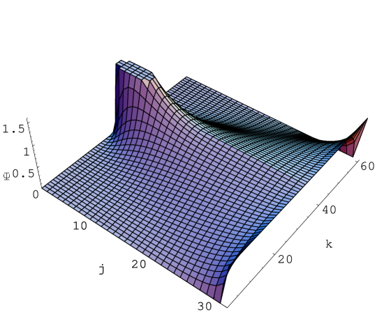
Figure 2: The solution of pulsar equation with Scharlemann & Wagoner conditions shown in the compactified domain.

5 Discussion and summary

The new method of calculating source function seems to work well. For bigger grids we don’t presume they would improve the results qualitatively. We can repeat our calculations with Timokhin (tim05 ) boundary conditions.

In our solution the surface of $\Psi$ is smooth apart from the equatorial plane outside the light cylinder.
The introduction to the problem can be found in bkk06 .

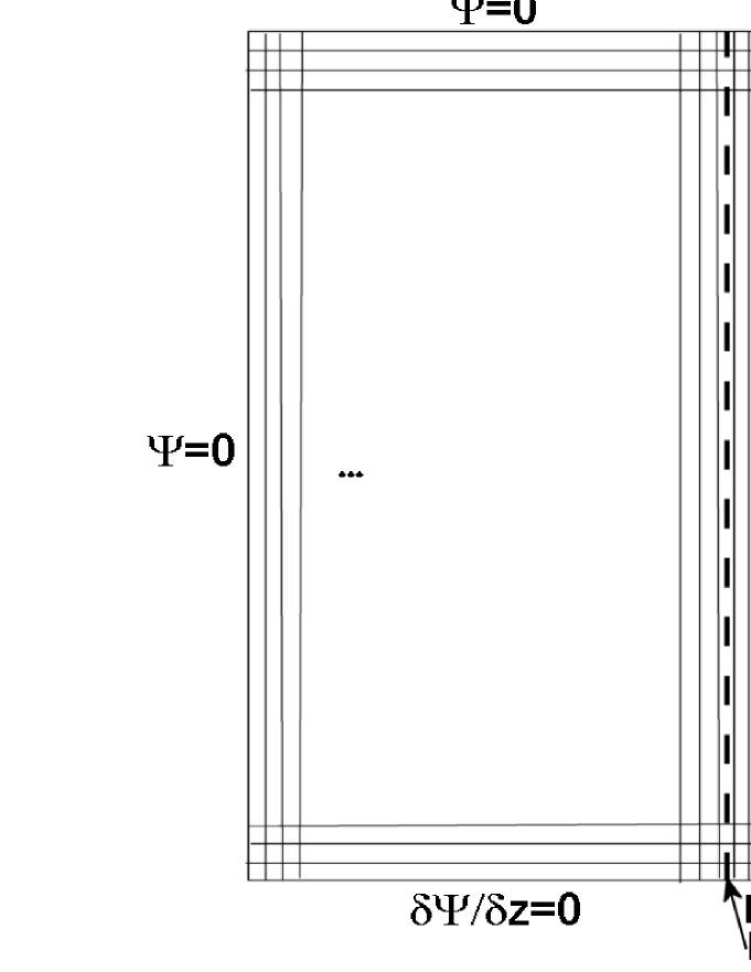
Figure 3: Compactified integration grid which covers whole physical space. The light cylinder which is singular surface of the pulsar equation is located between adjacent grid columns.

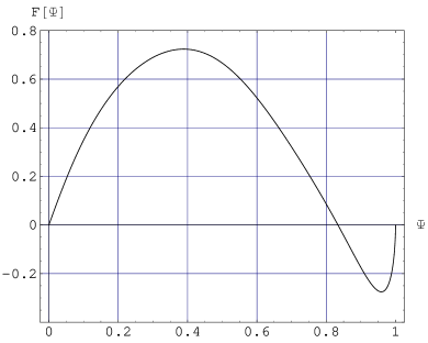
Figure 4: Source function $F(\Psi)$ found for $n=15$ and $m=6$.

References

- (1) Bratek, Ł., Kolonko, M., Kutschera, M.: Solutions of pulsar equation by finding the source term. Submitted to ApJ. (2006)
- (2) Contopoulos, I., Kazanas, D., Fendt, C.: The Axisymmetric Pulsar Magnetosphere. ApJ, 511, 351-358 (1999)
- (3) Goldreich, P., Julian, W.H.: Pulsar Electrodynamics. ApJ, 157, 869-880 (1969)
- (4) Gruzinov, A.: Power of an Axisymmetric Pulsar. PhysRevLett., 94, id. 021101 (2005)
- (5) Komissarov, S.S.: Simulations of axisymmetric magnetospheres of neutron stars. MNRAS, 367, 19-32 (2006)
- (6) Scharlemann, E.T., Wagoner, R.V.: Aligned rotating megnetospheres. I. General analysis. ApJ, 182, 951-960 (1973)
- (7) Spitkovsky, A.: Pulsar electrodynamics: a time-dependent view. Editors: Bulik, T., Rudak, B., Madejski, G., Astrophysical Sources of High Energy Particles and Radiation, Toruń 20-24 June 2005, pp. 253-256. AIP conference proceedings, 801 (2005)
- (8) Timokhin, A.N.: High resolution numerical modelling of the force-free pulsar magnetosphere. Editors: Bulik, T., Rudak, B., Madejski, G., Astrophysical Sources of High Energy Particles and Radiation, Toruń 20-24 June 2005, pp. 332-333. AIP conference proceedings, 801 (2005)
- (9) Timokhin, A.N.: On the force-free magnetosphere of an aligned rotator. MNRAS, 368, 1055-1072 (2006)