Parametric Strong Gravitational Lensing Analysis of Abell 1689

Abstract

We measure the mass distribution of galaxy cluster Abell 1689 within $0.3$ Mpc/h₇₀ of the cluster centre using its strong lensing effect on 32 background galaxies, which are mapped in altogether 107 multiple images. The multiple images are based on those of Broadhurst et al. (2005a) with modifications to both include new and exclude some of the original image systems. The cluster profile is explored further out to $\sim$ 2.5 Mpc/h₇₀ with weak lensing shear measurements from Broadhurst et al. (2005b).

The masses of $\sim$200 cluster galaxies are measured with Fundamental Plane in order to accurately model the small scale mass structure in the cluster. The cluster galaxies are modelled as elliptical truncated isothermal spheres. The scaling of the truncation radii with the velocity dispersions of galaxies are assumed to match those of i) field galaxies (Hoekstra et al., 2004) and ii) theoretical expectations for galaxies in dense environments (Merritt, 1983). The dark matter component of the cluster is described by either non-singular isothermal ellipsoids (NSIE) or elliptical versions of the universal dark matter profile (ENFW). To account for substructure in the dark matter we allow for two dark matter haloes.

The fitting of a single isothermal sphere to the smooth DM component results in a velocity dispersion of 1450${}^{+39}_{-31}$ km/s and a core radius of 77${}^{+10}_{-8}$ kpc/h while an NFW profile has a a virial radius of 2.86$\pm$0.16 Mpc/h₇₀ and a concentration of 4.7${}^{+0.6}_{-0.5}$.

The total mass profile is well described by either an NSIS profile with $\sigma$=1514${}_{-17}^{+18}$ km/s and core radius of $r_{c}$=71$\pm$5 kpc/h₇₀, or an NFW profile with C=6.0$\pm$0.5 and r₂₀₀=2.82$\pm$0.11 Mpc/h₇₀. The errors are assumed to be due to the error in assigning masses to the individual galaxies in the galaxy component. Their small size is due to the very strong constraints imposed by multiple images and the ability of the smooth dark matter component to adjust to uncertainties in the galaxy masses. The derived total mass is in good agreement with the mass profile of Broadhurst et al. (2005a) despite the considerable differences in the methodology used.

Using also weak lensing shear measurements from Broadhurst et al. (2005b) we can constrain the profile further out to r$\sim$2.5 Mpc/h₇₀. The best fit parameters change to $\sigma$=1499$\pm$15 km/s and $r_{c}$=66$\pm$5 kpc/h₇₀ for the NSIS profile and C=7.6$\pm$0.5 and r₂₀₀=2.55$\pm$0.07 Mpc/h₇₀ for the NFW profile.

Using the same image configuration as Broadhurst et al. (2005a) we obtain a strong lensing model that is superior to that of Broadhurst et al. (2005a) (rms of 2.7” compared to 3.2”). This is very surprising considering the larger freedom in the surface mass profile in their grid modelling.

1 Introduction

Abell 1689 at a redshift of 0.18 is one of the richest clusters of galaxies on the sky. Its closeness and richness should allow a straightforward mass determination using the gravitational lens effect on background galaxies, the dynamics of cluster members and the X-ray emission of the intra-cluster gas. Nevertheless, these methods have come up with strikingly different results in the past.

Observations with the Chandra (Xue & Wu, 2002) and XMM-Newton (Andersson & Madejski, 2004) satellites yield masses roughly a factor 2 lower than strong lensing measurements (e.g. Dye et al., 2001). The first line-of-sight velocity measurements of cluster members (Teague et al., 1990) had resulted in a velocity dispersion of $\sigma\approx 2355$ km/s, compared to a value of only $\sigma\approx 1028$ km/s for an isothermal fit to weak lensing measurements by, for example, King et al. (2002). Therefore the isothermal sphere velocity dispersion estimates of the cluster from strong lensing, X-ray and weak lensing analysis originally implied a mass estimate different at a factor of up to 5.

The apparently incompatible weak and strong lensing results for an isothermal sphere are most puzzling since both methods measure the (same) line-of-sight projected two dimensional surface mass density of the cluster. If parameters obtained with these two methods on different angular scales do not agree for a given mass profile, it implies that i) the assumed mass profile does not describe the true mass distribution at all, or ii) that one analysis (more likely the weak lensing analysis) suffers from underestimated systematic errors. Broadhurst et al. (2005a) have shown that this is the case for A1689, i.e. that in previous analyses the contamination of the ’background galaxies’ with cluster members could have biased the lensing signal of the background galaxies. Their background galaxies show (compared to Clowe & Schneider (2001); King et al. (2002)) a factor of roughly two higher lensing signal on large scales and make the order of magnitude mass estimate in the weak and strong lensing analysis agree.

The discrepant results from the cluster dynamics and the X-ray data relative to the strong lensing analysis can potentially be explained, if some assumptions in the interpretation of galaxies’ dynamics and the gas X-ray emissivity, i.e. having one spherically symmetric isothermal structure in dynamical equilibrium, are not valid. Indeed, Girardi et al. (1997) identified three substructures (using spectroscopic data from Teague et al. (1990)) in Abell 1689 which are well separated in velocity but overlap along the line of sight. This reduced the previous value of the cluster’s velocity dispersion from $2355$ km/s by Teague et al. (1990) to $1429$ km/s, a value in good agreement with strong lensing results. Evidence for substructure and merging was also found in velocity differences of X-ray emission lines and in X-ray temperature maps by Andersson & Madejski (2004). They pointed out that the (by a factor of two low) X-ray mass estimate would double if two equal mass structures along the line-of-sight are responsible for the X-ray emission in stead of just one structure. The X-ray surface brightness map, however, and the weak lensing data of A1689 indicate an almost circular (2D projected) mass distribution centred on the cD galaxy. This is not necessarily contradicting the substructure results summarised above, as long as the two major contributions in mass are on the same line of sight, and each of them is a fairly relaxed structure. The issue of relax/unrelaxed systems and the cluster X-ray temperature - mass relation is studied in 10 X-ray luminous galaxies by Smith et al. (2005) using Chandra X-ray and weak and strong lensing. They find that a large fraction of their clusters are experiencing, or recovering from, a cluster-cluster merger and that the scatter in the cluster X-ray temperature - mass relation is significantly larger than expected from theory.

The current status of the strong and weak lensing, the dynamical and the X-ray mass estimates for A1689 are defined by the works of Broadhurst et al. (2005a), Broadhurst et al. (2005b), Girardi et al. (1997) and Andersson & Madejski (2004) respectively. The mass estimates agree well with the exception of the still low X-ray mass estimate. The X-ray mass can be brought in line with the masses from other methods if two equal mass substructures along the LOS are responsible for the X-ray emission (Andersson & Madejski, 2004).

Broadhurst et al. (2005b) also carried out a combined strong and weak lensing analysis. They rule out a softened isothermal profile at a 10-$\sigma$ level. According to their work, a universal dark matter profile (NFW) with a concentration of $C=13.7^{+1.4}_{-1.1}$ and a virial radius of $r_{vir}=2.04\pm 0.07~{}Mpc/h_{100}$ fits the shear and magnification based on weak and strong lensing data well. They point out that the surprisingly large concentration for A1689 together with results from other clusters could point to an unknown mechanism for the formation of galaxy clusters. The strong rejection of an isothermal sphere type profile has also been reported in galaxy cluster Cl 0024+1654 by Kneib et al. (2003) who probed the cluster profile to very large clustercentric radius (5 Mpc).

Oguri et al. (2005) however have demonstrated that halo triaxiality can lead to large apparent central concentrations, if these haloes are analysed assuming spherical symmetry. This is because a highly elongated structure along the LOS imitates a high central density if investigated in projection only. Allowing for triaxiality the central concentration is less well constrained and not in disagreement with results from numerical simulations of cluster mass profiles.

In our work we want to address the following points:

• Does one obtain the same mass profile with an analysis of the strong lensing effect using a different method? We concentrate on differences between grid method used by Broadhurst et al. (2005a) and our parametric method.

• Are mass profiles from weak (WL) and strong (SL) lensing at all compatible with each other, or does the combination of both observations already rule out an NFW or an isothermal profile?

• How much does the large concentration and the level of compatibility of the WL and SL results depend on the values of two outermost WL shear data points?

• How good is the relative performance of an isothermal sphere vs. an NFW profile, based on both the strong and weak lensing analyses?

We aim to investigate all these points with parametric cluster models. Our basic assumptions are that substructure follows galaxies and the cluster mass can be described by mass associated with the galaxies (both luminous and dark) plus a smooth component. The multiple image configurations determine if there are one or more of these smooth components necessary, e.g. two haloes of similar mass like in A370 (see e.g. Kneib et al. (1993); Abdelsalam et al. (1998)) , or a massive halo plus less massive, group-like components.

We describe the smooth component by 2 parametric halo profiles. Deviations from symmetry are accounted for by elliptical deflection angles (ENFW) or potentials (NSIE) depending on the model. The first halo profile is the so called universal dark matter profile (hereafter NFW profile), an outcome of numerical simulations of cold dark matter cosmologies (Navarro et al., 1996). The second is a non-singular isothermal ellipsoid (NSIE) which naturally reproduces the observed flat rotation curves of both late and early-type galaxies.

The profiles of cluster galaxies are described with an elliptical truncated isothermal sphere profile (Blandford & Kochanek, 1987) whose velocity dispersions are determined using both Fundamental-Plane and Faber-Jackson relations.

Provided a range of plausible radial mass profiles are tested with parametric halo profiles significantly better performance of grid methods, like the one used by Broadhurst et al. (2005a) (also Diego et al. (2005a, b)), can give clues to the existence of dark matter substructure not traced by galaxies (dark mini haloes) if these dark haloes are numerous/massive enough to influence the lensing observables on a relevant level. The difference can also result from the details of a particular modelling, e.g. the treatment of the cluster galaxy component and in the dark matter profiles used in modelling the smooth DM of the cluster.

In section 2 we give a brief summary of the data and data analysis used in this paper. Section 3 describes our method to obtain the best fitting lensing models, results are given and discussed in section 4. We draw conclusions in section 5.

The cosmology used throughout this paper is $\Omega_{m}$=0.30, $\Omega_{\Lambda}$=0.70 and H₀=70 km/s/Mpc, unless otherwise stated.

2 Data and Data Analysis

We have used archived optical HST (WFPC2 and ACS) data in filters F555W and F814W (WFPC2) and F475W, F625W, F775W and F850LP (ACS). A summary of the data can be seen in Table 1. The relatively wide field-of-view (202”x202”) and high resolution (pixelscale 0.05”) of ACS allow us to probe A1689 over the area where most of the multiple images are formed. WFPC2 data are used to further constrain the photometric redshifts in the central region of A1689 covered by the observations.

2.1 Data Reduction

2.1.1 HST - WFPC2

The WFPC2 data in filters F555W and F814W come from HST proposal 6004 by Tyson. We use pipeline flatfielded images which were combined using iraf tasks in combination with psf fitting cosmic ray rejection algorithms developed in house (Gössl & Riffeser, 2002). The steps of data reduction were as follows. First all features with FWHM less than 1 pixel and a high signal to noise were marked as cosmic rays and not used in any further analysis. In the second step the four chips of each WFPC2 exposure were transformed to a single coordinate system. In this step both the geometrical distortions of the WFPC2 chips as well as translation and rotation between the different CCDs and exposures were taken care off. The description of Holtzman et al. (1995) was used to remove the geometrical distortions. The different chips have slightly different photometric zeropoints and before the images were stacked all the images were normalised to the zeropoint of the planetary camera. The stacking was done by taking a kappa-sigma clipped mean of each pixel. It was found during the reduction process that the two stage cosmic ray rejection was necessary in order to remove all the cosmic rays efficiently. Most of the cosmic rays were removed by psf- fitting in the first stage and larger pointlike cosmic rays were removed in the stacking stage by the kappa-sigma clipping.

Table 1: A summary of the data used in this study.

Filter	t (ks)	# of exposures	psf (″)
F555W (WFPC2)	44.2	17	0.17
F814W (WFPC2)	5.0	5	0.20
F475W (ACS)	9.5	8	0.11
F625W (ACS)	9.5	8	0.10
F775W (ACS)	9.5	8	0.10
F850LP (ACS)	16.6	14	0.11

2.1.2 HST - ACS

The advanced Camera for Surveys has a larger field of view than WFPC2 at a similar resolution. The data in filters F475W, F625W, F775W and F850LP come from HST proposal 9289 by Ford. The ”on the fly re-processing” (OTFR) provides flatfielded and calibrated data. The individual exposures were transformed to a common coordinate system using PyDrizzle in pyraf. The cosmic rays were again removed in 2 stages as with the WFPC2 data.

2.2 Object Catalogues

The object catalogue was obtained with SExtractor (Bertin & Arnouts, 1996). To optimise the extraction parameters of Sextractor - detection threshold and number of contiguous pixels - a procedure similar to that in Heidt et al. (2003) was followed. Sources were detected from a signal-to-noise weighted sum of the four ACS filters. The photometry for the detected sources was then done in all filters. Output of SExtractor used later in the lensing model include total and aperture photometry as well as source ellipticities and their position angles.

2.3 Spectroscopic redshifts

The redshift data are collected from several published studies of Abell 1689 (Girardi et al. 1997, Balogh et al. 2002, Duc et al. 2002, Golse 2002). In total 84 spectroscopic redshifts were available in the ACS field of A1689. Except Golse, these studies concentrate on the line-of-sight velocities of the cluster members in order to obtain the velocity dispersion and hence an estimate of the dynamical mass of the cluster. The redshift information is used to get secure cluster members for the lensing analysis, to exclude galaxies which are not part of the cluster and to compare photometric redshifts with spectroscopic ones.

2.4 Photometric redshifts

Figure 1: Comparison between spectroscopic and photometric redshifts. Notice how the reddest cluster ellipticals have been pushed to higher redshifts to compensate for the relative blueness of the model elliptical SED in the SED library used to compute the photometric redshifts. Filled symbols show the most likely redshift, open symbols the second most likely for the objects where it is closer to the true redshift.

Figure 2: Photometric redshift distribution of objects in the field of A1689. The cluster is clearly visible as a peak at z$\sim$0.2. The inlaid figure shows objects considered as cluster galaxies. In a number of cases the 4000 $\AA$ break of cluster galaxies was misinterpreted as Lyman break and hence a redshift z$\sim$3 was assigned (see text for details).

We have calculated photometric redshifts using the method described in Bender et al. (2001). For the central regions we were able to use all 6 filters, otherwise only the 4 available ACS filters were used. Comparison between photometric redshifts and available spectroscopic ones is shown in Figure 1. Unfortunately spectroscopic redshifts are not numerous and those that exist are mainly for cluster members. The model elliptical galaxy in the SED library used to calculate the photometric redshifts is bluer than the reddest cluster members and hence the cluster galaxies are pushed to redshifts slightly higher than that of the cluster. The slope of the cluster redsequence causes the large spread in photometric redshifts of the cluster members. The photometric redshift distribution of all objects is shown in Figure 2. The cluster appears as a narrow peak at z$\sim$0.2 on the redshift histogram. Objects at z$\sim$3-4 are either gravitationally lensed background galaxies or cluster galaxies whose 4000 $\AA$ break was misidentified as Lyman break. This places them to redshifts $\sim$3. To clearly discriminate between the two breaks we would need both redder and especially bluer filters than the ones available. This confusion is not important in our case since photometric redshifts are used to constrain redshifts of the multiple images. For these the low redshift peak can be excluded because gravitational lensing is inefficient if the background source is close to the lens.

3 Lensing Models

In this section we describe how the lensing models of A1689 were constructed; the different mass components of the cluster, the multiple image systems and the optimisation of model parameters. The lensing profiles are described in detail in appendix A.

3.1 Cluster Galaxy Component

The cluster galaxies were selected using the redsequence method supported by spectroscopic redshifts where available. The spectroscopic data are taken from Girardi et al. (1997) (using data from Teague et al. (1990)), Balogh et al. (2002) and Duc et al. (2002). We have excluded 6 objects from the cluster catalogue obtained with the redsequence method based on fore/background objects listed in Balogh et al. (2002) and Duc et al. (2002). Fig. 3 shows a colour-magnitude diagramme of the cluster. We chose to use filters F475W and F775W from the ACS observations as the cluster redsequence is seen particularly clearly in these two filters. Galaxies included in the lensing analysis are marked by triangles in Figure 3. Solid triangles show the galaxies which have been spectroscopically confirmed to be cluster members in one or more of the referred papers. To find more members a redsequence in the CM diagramme was determined by fitting a line to the bright end of the redsequence. Those galaxies whose F475W-F775W colour deviated by less than 0.3 magnitudes from the fitted sequence were included as cluster members (region between the two inclined dashed lines in Figure 3).

Figure 4 shows the positions of cluster members in the field of A1689 (using the same symbols as in Figure 3).

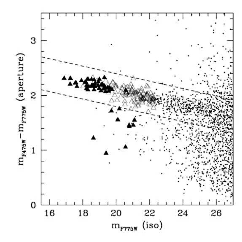
Figure 3: Cluster redsequence in ACS F475W/F775W colour-magnitude diagramme. The solid triangles represent cluster galaxies with spectroscopic redshifts, open triangles all other objects which were considered as cluster members in the lensing analysis. The remaining objects are represented by dots. A clear cluster redsequence can be seen. See section 3.1 for details on the selection criterion for cluster membership.

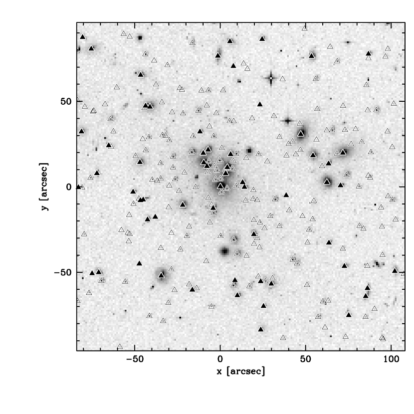
Figure 4: Positions of cluster galaxies in the field of Abell 1689. The symbols correspond to those in Fig. 3. Origin of the coordinate system is on the central cD galaxy. The box width is 200” (corresponding to $\sim$625kpc at z=0.18).

The cluster galaxies were modelled with an elliptical BBS profile (see appendix A for further details). We have treated the two parameter profile as a one parameter profile by assuming that $s=s(\sigma)$. We find the fit to multiple images with a galaxy component described by the values for $s_{*}$ (=185 $h^{-1}$ kpc) and $\sigma_{*}$ (=136 km/s) and the scaling ($s=s_{*}\times(\sigma/\sigma_{*})^{2}$) found for galaxies in the Red-Sequence Cluster Survey (Hoekstra et al., 2004) is very poor. This means that the galaxy haloes in A1689 must be significantly stripped. The stripping of galaxies in cluster environment has been reported earlier by e.g. Natarajan et al. (1998, 2002) who have used galaxy–galaxy lensing in clusters to study the propertias of galaxy haloes in 6 clusters at redshifts Z=0.17-0.58. They found strong evidence for tidally truncated haloes around the galaxies compared to galaxies in the field.

We base our models for the tidal stripping of galaxies on observational work by Hoekstra et al. (2004) for galaxies in the field ($s\propto\sigma^{2}$) and theoretical expectations for galaxies in cluster environment ($s\propto\sigma$) (Merritt, 1983). We only take the scaling of the truncation radii with the velocity dispersions of the galaxies from the aforementioned works and find the normalisation of the truncation radius, $s_{*}$, to fit the multiple images. The two scaling laws adopted in the paper are then 1) $s=s_{*}\times(\sigma_{gal}/136km/s)^{2}$ and 2) $s=s_{*}\times(\sigma_{gal}/136km/s)$, where for both scaling laws and all Models we have found the $s_{*}$ that best reproduces the observed multiple images. The scaling law for the truncation of galaxies in cluster environment will be treated in more detail in a forth coming publication (Halkola et al., 2006 in preparation).

The positions, ellipticities (of surface brightness) and position angles were taken from SExtractor output parameters. The velocity dispersions of cluster galaxies were determined mostly using the Fundamental Plane. For a small number of galaxies also the Faber-Jackson relation was used.

3.1.1 Central Velocity Dispersions of Cluster Galaxies & Halo Velocity Dispersions

The Fundamental Plane (hereafter FP) links together, in a tight way, kinematic (velocity dispersion), photometric (effective surface brightness) and morphological (half light radius) galaxy properties (Dressler et al., 1987; Djorgovski & Davis, 1987; Bender et al., 1992). We assume that the central velocity dispersions of a galaxy, as derived from the FP, is equal to the halo velocity dispersion, and that mass in disk can be neglected.

The FP relation allows us to estimate the velocity dispersion of galaxies more accurately than the standard Faber-Jackson relation approach (Faber & Jackson, 1976). We model the 2–dimensional light profiles of cluster galaxies with PSF–convolved Sersic (Sersic, 1968) profiles using two packages, GALFIT (Peng et al., 2002) and GIM2D (Simard et al., 1999), to have a better handle on the systematics. The analysis was performed on the F775W ACS image. 176 objects with AB magnitudes brighter than 22 were fitted. The point spread function used to convolve the models was derived by stacking stars identified in the field. The results coming out from the two completely different softwares agree very well.

In order to be able to use a FP determination for cluster galaxies at redshift $\sim 0.2$ in restframe Gunn r filter (Jørgensen et al., 1996; Ziegler et al., 2001; Fritz et al., 2005), all the observed F775W_AB surface brightnesses (extinction corrected) were converted to restframe Gunn r_GT ones and corrected for the cosmological dimming. Since the observed F775W passband is close to restframe Gunn r at the redshift of A1689, the conversion factor between observed F775W and restframe Gunn r is small.

The mean observed surface brightness within $r_{e}$ is:

$$\langle\mu_{e}\rangle_{F775W}=F775W_{observed}+2.5\log(2\pi)+5\log(r_{e})-10\log(1+z),$$ (1)

where the last term corrects for the dimming due to the expansion of the Universe. It is then converted to restframe Gunn r_GT by:

$$\mathrm{\langle\mu_{e}\rangle}_{r}=\mathrm{\langle\mu_{e}\rangle}_{F775W}-A_{F775W}+K(r,F775W,z)+GT_{corr},$$ (2)

The Galactic extinction correction $A_{F775W}$ is calculated from the list of A/E(B-V) in Table 6 of Schlegel et al. (1998), along with their estimate of E(B-V) calculated from COBE and IRAS maps as well as the Leiden-Dwingeloo maps of HI emission. We adopted for $A_{F775W}$ a value of 0.06.

The ”k-correction colour”, K(r,F775W,z), is the difference between rest frame Gunn r and observed F775W magnitude and includes also the $2.5\log(1+z)$ term. It was obtained by using an elliptical template from CWW (Coleman et al., 1980) and synthetic SEDs obtained for old stellar populations (10 Gyr, i.e. z_f = 5 observed at z=0.2) with the BC2003 Bruzual and Charlot models (Bruzual & Charlot, 2003). All models give a conversion factor of approximately 0.174. The correction needed to pass from the AB photometric system to the Gunn&Thuan system is GT${}_{\textrm{corr}}\approx 0.17$ .

We used the FP coefficients from Fritz et al.. For the Gunn r band then

$$1.048*\log R_{e}=1.24*\log\sigma-0.82*\langle I\rangle_{e}+ZP_{FPr},$$ (3)

where the $\langle I\rangle_{e}$ term, i.e. the mean surface brightness in units of L_⊙/pc², is given for the Gunn r band by the equation:

$$\log\langle I\rangle_{e}=-0.4(\langle\mu_{r}\rangle_{e}-26.4).$$ (4)

The zero–point of the FP $ZP_{FPr}$ is a quantity changing with both the cluster peculiarity and, mainly, with the cluster redshift. We used for $ZP_{FPr}$ the value published in Fritz et al. (2005). Their study was focused on A2218 and A2390, two massive clusters at almost the same redshift as A1689. They applied a bootstrap bisector method in estimating the $ZP_{FPr}$ and relative uncertainties, finding a value of 0.055$\pm$0.022.

Finally, we inserted the values derived from our morphological fitting procedures into the FP relation. The uncertainties on the derived velocity dispersions were estimated by taking into account the errors on the morphological parameters, the propagated photometric uncertainties, the error on the $ZP_{FPr}$ value and the intrinsic scatter of the FP relation, which gives the main contribution. We found that an estimate of 0.1 in log($\sigma$) is a good value for the total uncertainty in velocity dispersion for objects having a velocity dispersion greater than 70 km/s. For lower velocity dispersions down to 24 km/s, we assumed an overall uncertainty of 0.2 dex. The fitted parameters for the 80 most massive galaxies are tabulated in Table 7.

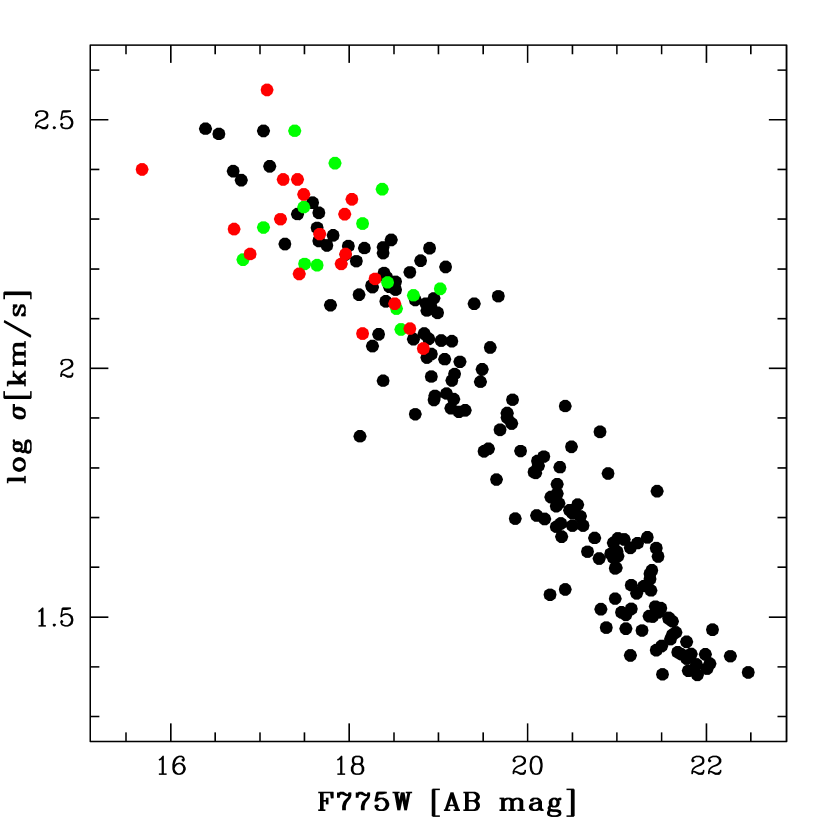
Figure 5: Total observed magnitude - $\sigma$ relation for three z$\sim$0.2 clusters. Red points are measured values taken from Ziegler et al. (2001) for A2218 (z=0.18), green points are values taken from Fritz et al. (2005) for A2390 (z=0.23) and full (empty) black points refer to the velocity dispersion estimates obtained in this paper for A1689 using the GIM2D (GALFIT) morphology. The literature values have been transformed to F775W_AB magnitudes by applying relatively small colour terms (0.04,-0.4) and the AB correction (0.4).

Additionally, we have obtained the velocity dispersions of 26 galaxies using the Faber-Jackson relations derived using the 176 galaxies for which we have obtained the velocity dispersions via FP. These are all faint galaxies with $\sigma<60km/S$.

The Einstein-radius of an isothermal sphere can then be written as $\theta_{E}=1.4^{\prime\prime}(\sigma/220km/s)^{2}$ D, where D is a geometrical factor of order unity depending on redshifts of the objects and cosmology (0.78 $<$ D $<$ 0.92 for 1 $<z_{s}<$ 6 and our adopted cosmology). Cluster members with $\sigma>24~{}\mathrm{km/s}$ were included in the galaxy component of the cluster. This limit is somewhat arbitrary and below the luminosity limit where FP and FJ are determined. An Einstein radius smaller than the pixel size of the ACS ensures that all galaxies which could significantly affect image morphologies locally are included when external shear and convergence from the other cluster galaxies and the cluster halo are present.

3.1.2 Ellipticities of Cluster Galaxies and Their Haloes

Blandford & Kochanek (1987), Kormann et al. (1994) and others have noted that for elliptical potentials the accompanying surface mass density can have negative values. We have used elliptical potential for our NSIE profile since it is straightforward to implement (all parameters of interest can be calculated from the analytic derivatives of the potential). An alternative approach is to have an elliptical mass distribution as demonstrated by Kormann et al. (1994) but the expressions for $\alpha\textrm{, }\kappa\textrm{ and }\gamma$ are considerably more complicated.

For the ENFW and BBS profiles we have introduced the ellipticity to the deflection angle, see appendix A for details and references. The effect of using an elliptical deflection angle instead of an elliptical mass distribution is shown in Figure 6. The ellipticities of the mass distributions were estimated by fitting an ellipse to $\kappa$=0.2 isodensity contours for both BBS (top) and ENFW (bottom) haloes with 6 different ellipticities (0, 0.05, 0.1, 0.15, 0.2 and 0.25). On the right panel a quarter of the $\kappa$=0.2 isodensity contour for different profile ellipticities are drawn in solid. Dashed lines show the best fit ellipses. For the BBS model the isodensity contours start to deviate from an ellipse at $\epsilon_{defl}>$0.15, where the contours first appear boxy before turning peanut shaped. For the ENFW profile the contours are only slightly peanut shaped at $\epsilon_{pot}$=0.25. Left panels of Figure 6 show how the ellipticity of mass deviates from $\epsilon_{kappa}$=2$\epsilon_{defl}$ and $\epsilon_{kappa}$=3$\epsilon_{defl}$ lines shown dashed. We have assumed that light and mass have the same ellipticity and used the relation in Figure 6 to convert the measured galaxy ellipticities ($\epsilon_{kappa}$) to BBS model ellipticities ($\epsilon_{defl}$). A histogram of the ellipticities of the included cluster galaxies are shown in Figure 7.

Figure 6: Ellipticity of surface mass density vs. profile ellipticity (in deflection angle) for the two profiles (BBS is on the top two panels and ENFW on the bottom two). The ellipticity of $\kappa$ is estimated by fitting an ellipse to lines of constant surface mass density. Right panels show $\kappa$=0.2 isodensity contours in solid and fitted ellipses in dashed lines. Profile ellipticities are 0.0, 0.05, 0.10, 0.15, 0.20, 0.25 and increase from bottom to top. The curves have an offset of 0.25 in b for clarity. Left panels show $\epsilon_{kappa}$ as a function of profile ellipticity $\epsilon_{defl}$. The dashed lines are $\epsilon_{kappa}$=3 $\epsilon_{defl}$ and $\epsilon_{kappa}$=2 $\epsilon_{defl}$ lines.

Figure 7: A histogram of the ellipticities, $\epsilon_{defl}$, for the BBS profiles used to model the cluster galaxies. Most of the galaxies have an ellipticity well below 0.15 where the isodensity contours of surface mass density start to appear peanut shaped.

3.2 Dark Matter Not Associated with Galaxies

Different studies have shown that Abell 1689 is not a simple structure with only one component. In an early strong lensing analysis of A1689 Miralda-Escude & Babul (1995) assumed two halo components based on the distribution of galaxies. Girardi et al. (1997), on the other hand, spectroscopically identified three distinct groups in Abell 1689. More recently Andersson & Madejski (2004) have also found evidence for substructure and possible merger in X-ray data. This prompted us to model the cluster dark matter in A1689 with two dark matter haloes. The use of more haloes in the modelling is not desired since this increases problems related to a large number-of free parameters; larger parameter space to explore, increased difficulty of finding global minimum and degeneracies between the free parameters. Both haloes have 6 free parameters: position (x,y), ellipticity, position angle and in the case of NSIE profile velocity dispersion $\sigma$ and core radius $r_{c}$ and for the NFW profile virial radius $r_{200}$ and concentration parameter C.

For all the following modelling we have constrained the first halo to reside within 50” in x and y from the cD galaxy in order to reduce the volume of the parameter space and to reduce the degeneracy between the parameters of the two haloes. We do not want to tightly connect the halo with any of the galaxies but use the position of the cD as a first guess for the position of the cluster centre. This is supported by X-ray maps of Abell 1689 (Xue & Wu, 2002; Andersson & Madejski, 2004) as well as weak lensing studies (King et al., 2002) which place the centre of the mass distribution very near the cD galaxy. The position of the second halo was initially set to coincide with the visually identified substructure to the north-east of the cluster centre but was left unconstrained in the optimisation.

3.3 Multiple Images & Arcs

It is evidently of great importance for the modelling to find as many multiple images as possible. The colour and surface brightness of an object are unaffected by gravitational lensing and we have hence used the colour, surface brightness and the morphology of the images to identify multiple image systems. We have first identified arcs and obvious multiple images which were then used to find an initial set of halo parameters. Initial constraints include images from image systems 1, 3, 4, 5, 6, 12 and arcs that contain images systems 8, 14, 20 and 32. A model based on these images could now be used to search for more images for the existing image systems as well as new image systems which could be included in the model and constrain the model parameters further. New images were searched for by looking for image positions whose source lies within a specified distance, e.g. 5”, from the source of an existing image. This method is basically the same as described in Schramm & Kayser (1987) and Kayser & Schramm (1988).

The images we have found are with a few exceptions also identified in the pioneering work of Broadhurst et al. (2005a) and essentially form a subset of their images. For our analysis we have merged the two image catalogues to obtain a catalogue of 107 multiple images in 32 image systems one of which is an long arc. In the merging we have split the image system 12 from Broadhurst et al. (2005a) to two separate systems (12 and 13) with 2 additional images from our catalogue. The splitting includes separating two images with the same spectroscopic redshift into two different image systems. We have done this based on the morphology of the images and our lensing models and we believe these to originate from 2 different sources. Also Seitz et al. (1998) in their analysis of cluster MS-1512 reported two sources at the same redshift. In the case of MS-1512 Teplitz et al. (2004) used near-infrared spectroscopy to confirm that the sources were indeed separate with a difference of only 400 km/s in velocity (0.0013 in redshift). To positively identify a set of images to originate from a single source is very difficult without extremely accurate spectroscopy or obviously the same (complex) morphology. The field of A1689 has a vast number of images that can potentially be erroneously assigned to any multiple image system. In our work we have rather excluded an image than include it in an image system. For this reason we have also excluded image system 20 from Broadhurst et al. (2005a) from our analysis. Image systems not used by Broadhurst et al. (2005a) are systems 31 and 32, a system with 2 images and a long arc respectively.

Of the images systems used 8 have an even number of images. The missing images in these cases are always demagnified and based on the lensing models mostly expected to lie near a galaxy making their identification very difficult.

In Figure 8 we show all the multiple images used in this study. More details, such as positions and redshifts, of the image systems, arcs and images can be found in Appendix C Tables 8 and 9 as well as Broadhurst et al. (2005a).

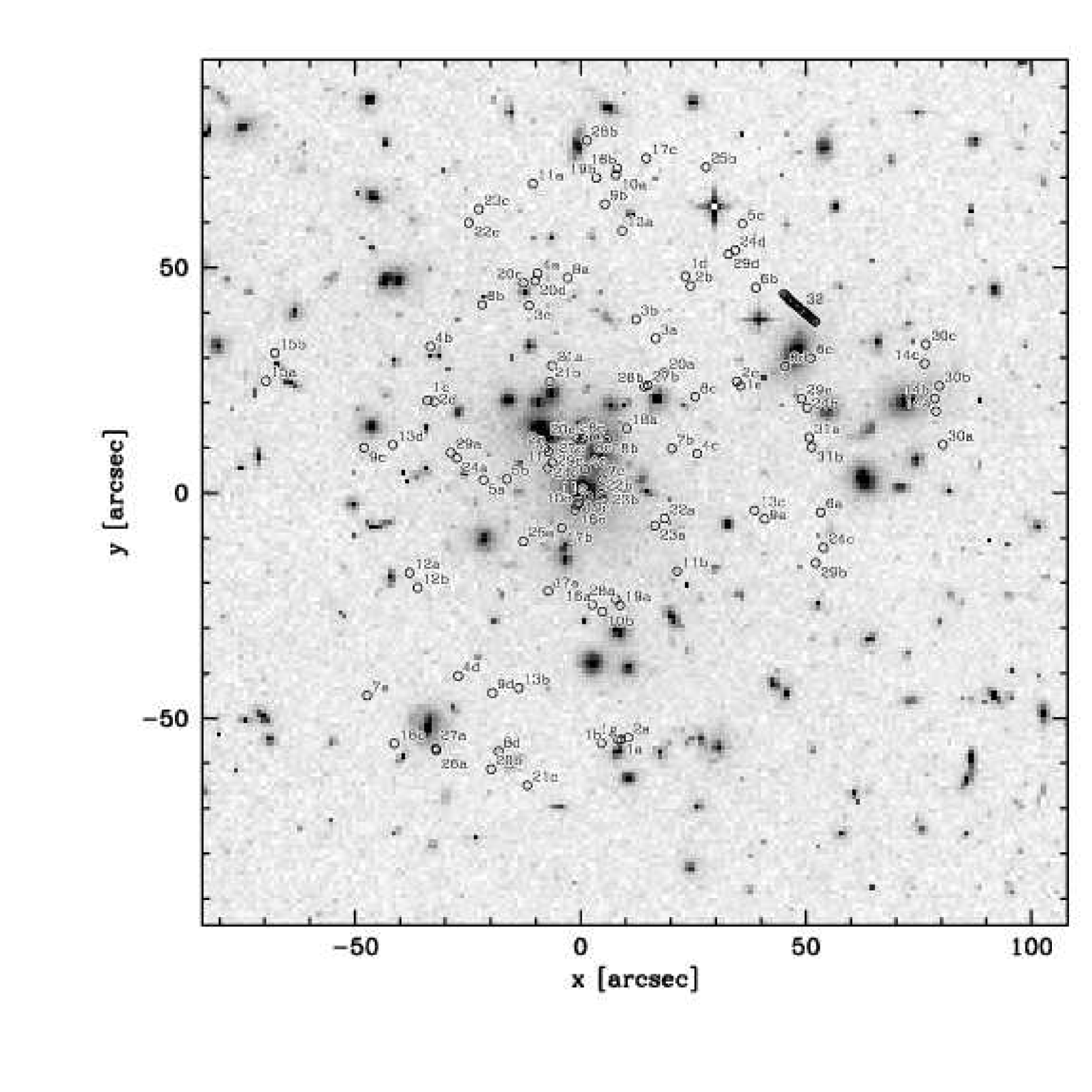
Figure 8: Positions of multiple images used in constraining the model parameters. The images from each multiple image system have the same number, the images within an image system are coded with letters. The box side is $\sim$600 kpc with our cosmology.

A comparison between photometric redshifts from this work and those of Broadhurst et al. (2005a) is shown in Figure 9. The overall agreement is very good. The one object with a z$\sim$1 from Broadhurst et al. (2005a) and z$\sim$3.4 from this work belongs to image system 1 and is one of the few objects with a spectroscopic redshift (z_spec=3.0).

Figure 9: A comparison of photometric redshifts of multiple images from this work to those from Broadhurst et al. (2005a). The correspondence is very good and for all objects within the errors. The one object with a z${}_{phot}\sim$1 from Broadhurst et al. (2005a) and z${}_{phot}\sim$3.4 from this work has a spectroscopic redshift of z${}_{spec}=$3.04.

In Figure 10 we show the photometric redshift probability density of the 5 multiple image systems with a spectroscopically known redshift. In the figures the different colours represent the probability densities of individual multiple images of the system. In most of the cases the spectroscopic and photometric redshifts agree very well. Only image systems 10 and 12 have a broad photometric redshift probability density distribution.

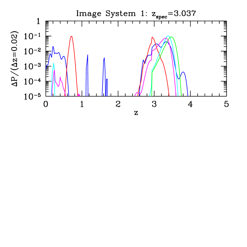
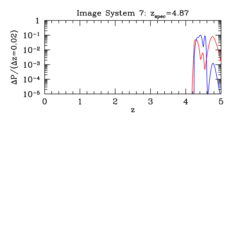
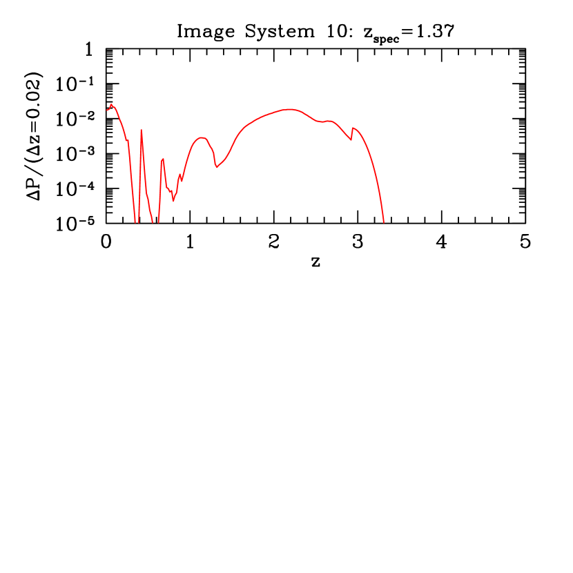
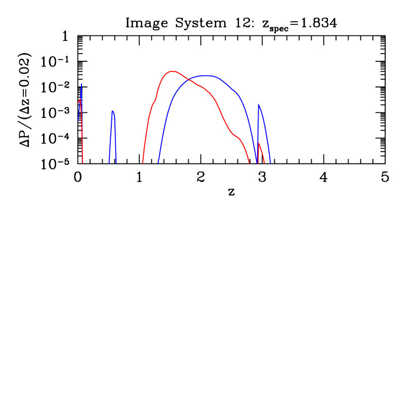
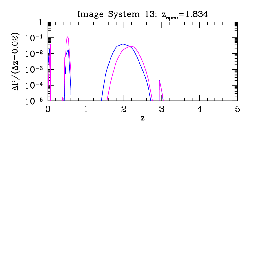
Figure 10: Photometric redshift probability density for the 5 image systems where spectroscopic redshift is known for at least one of the images in the system. In each panel the coloured thin lines represent individual redshift probability densities for the images in the system. Only image systems 10 and 12 have a broad photometric redshift probability density distribution, the other spectroscopic redshifts are recovered well.

The lensing power of a cluster depends on the ratio ${D_{ds}/D_{s}}$, where $D_{ds}$ is the angular diameter distance between the cluster and the source and $D_{d}$ is the angular diameter distance of the cluster. In Figure 11 we show the power of a lens at redshift 0.18 for different source redshifts. Vertical lines in Figure 11 show the range of allowed D_ds/D_s ratios for the image systems with photometric redshifts. The five squares mark the image systems with known redshifts (two have the same redshift). The D_ds/D_s ratio can be well constrained by photometric redshifts alone. With the help of the five spectroscopic redshifts we can very accurately separate the geometric factor from the deflection angle allowing us to constrain the cluster mass tightly.

Figure 11: The lensing power of a cluster depends on the ratio ${D_{ds}/D_{s}}$, where $D_{ds}$ is the angular diameter distance between the cluster and the source and $D_{d}$ is the angular diameter distance of the cluster. This ratio flattens rapidly for redshifts larger than 0.5 (for a cluster at redshift 0.18). In the figure we show the allowed ${D_{ds}/D_{s}}$ ratios of the different multiple image systems. The squares indicate objects with spectroscopic redshifts. Since ${D_{ds}/D_{s}}$ varies only little for z$>$2 the redshifts of sources are not of great importance. The spectroscopic redshifts are important in fixing the overall mass scale.

3.4 Finding Optimal Model Parameters

Goodness of fit in strong gravitational lensing can be quantified in two ways. The proper way is to calculate a $\chi^{2}$ in the image plane, i.e. how far an image predicted by a model is from the observed one. In calculating the positions of predicted images of an image system we assume that the images of a system originate from the average source of the images. The expression for an image plane $\chi^{2}$ is then

$${\chi}^{2}=\sum_{k}\sum_{i}{|\vec{\theta}_{k,i}-\vec{\theta}_{i}(<\vec{\beta}_{k,i}>)|^{2}\over\sigma_{k}^{2}},$$ (5)

where $\vec{\theta}_{k,i}$ is the position of image i in image system k and $\vec{\theta}_{i}(<\vec{\beta}_{k,i}>)$ is the predicted image position corresponding to image at $\vec{\theta}_{k,i}$ from mean source of system k at $<\vec{\beta}_{k,i}>$ and $\sigma_{k}$ is the error in image positions for system k (estimated to be 1 pixel for all images).

Calculating image plane $\chi^{2}$ is unfortunately very time consuming since the lens equation needs to be inverted numerically. An additional complication is that for some values of the model parameters not all observed images necessarily exist. This means that an image plane $\chi^{2}$ does not necessarily converge to the optimal parameters but is trapped in a local minimum.

Goodness of fit can also be estimated by requiring that all images of an image system originate from the same source and hence minimise the dispersion of the source positions. The problem in this case is that the errors are measured in the image plane and do not necessarily represent the errors in source positions. We take account of this by rescaling errors in the image plane with local magnification. Rescaling by magnification largely avoids bias towards cluster parameters with high magnification (large core radius for the NSIE model or small concentration for ENFW model). The source plane $\chi^{2}$, $\widetilde{\chi}^{2}$, can be written in the following way,

$$\widetilde{\chi}^{2}=\sum_{k}\sum_{i}\sum_{j>i}{|\vec{\beta}_{k,i}-\vec{\beta}_{k,j}|^{2}\over\sigma_{k,i}^{2}/\mu_{k,i}+\sigma_{k,j}^{2}/\mu_{k,j}},$$ (6)

where $\vec{\beta}_{k,i}$ is the source position of image i in system k, $\sigma_{k,i}$ is the error in the corresponding image position and $\mu_{k,i}$ is the local image magnification.

The advantage of $\widetilde{\chi}^{2}$ over $\chi^{2}$ is that for every image position it is always possible to calculate a corresponding source position and so $\widetilde{\chi}^{2}$ can be calculated for all values of the model parameters making $\widetilde{\chi}^{2}$ converge well.

To find optimal model parameters we have first minimised $\widetilde{\chi}^{2}$ to obtain model parameters close to the optimal ones to ensure that the identified multiple images can be reproduced by the models. The optimal model parameters were then found by minimising $\chi^{2}$ properly in the image plane.

3.5 Degeneracies

Any multiple image system can only constrain the mass contained within the images. This leads to degeneracies in the derived surface mass profile: the so called mass sheet degeneracy states that if a given surface mass density satisfies image constraints then a new surface mass density can be found, by suitably rescaling this surface mass density and by adding a constant mass sheet, which satisfies image positions as well as relative magnifications equally well.

For haloes with variable mass profile this can also create a degeneracy between the parameters of the profile. For the NSIE model a high core radius can be compensated for by a larger velocity dispersion and for NFW a higher scale radius demands a lower concentration parameter.

These degeneracies can be broken if multiple image systems at different redshifts and at different radii can be found. Position of a radial critical line, and so radial arcs, depends critically on the mass distribution in the central regions and hence the core radius. On the other hand tangential arcs give strong constraints on the mass on larger scales. Well defined halo parameters can be determined by having radial arcs, a large number of multiple images at different redshifts and by minimising in the image plane.

4 Constructing Lensing Models

We have constructed in total 4 strong lensing models for the cluster. The mass distributions are composed of two components as described in the previous section: the cluster galaxies and a smooth dark matter component. They give us the best fitting NSIE and ENFW parameters for the smooth dark matter component and the mass profile of the different mass components as well the total mass profile of the cluster. With Models I and II we aim to establish a well defined total mass profile for the cluster using the multiple image positions and the photometric redshifts of the sources. The difference between Models I and II is in the scaling law used for the cluster galaxies. Model I assumes a $s\propto\sigma^{2}$ law where as for Model II we use $s\propto\sigma$ law. Models Ib and IIb replicate the setup of Broadhurst et al. (2005a) and with these we want to compare results with our parametric models to the their more flexible kappa-in-a-grid model. For Models Ib and IIb we have used images from Broadhurst et al. (2005a) only and have left the photometric redshifts of the sources free as was done in Broadhurst et al. (2005a). We have kept the spectroscopic redshifts fixed as these help to define the mass scale of the cluster. The difference between Models Ib and IIb is again in the scaling law adopted.

In addition to the 4 strong lensing Models above we have also constructed 2 further Models in order to derive NSIS and NFW parameters of the total cluster mass profile and to facilitate the comparison of our results with earlier methods used to measure cluster masses, and numerical simulations. In Model III we have fitted a NSIS and an NFW profile to the total mass obtained with Models I and II. With Model IV we combine the strong lensing constraints from Model III and the weak lensing constraints from Broadhurst et al. (2005b) and derive accurate NSIS and NFW parameters for the total mass profile out to $\sim$15’ ($\sim$2.5 Mpc).

Most of the image systems are very well reproduced by the Models. Image systems 8, 12, 14, 15, 30, 31 and 32 are located close to critical lines where the image plane $\chi^{2}$ is difficult to calculate due to ill determined image positions from the models. For these image systems we have always calculated the $\chi^{2}$ in the source plane.

We quantify the quality of fit by the rms distance between an observed image position and one predicted by the models. For the images systems mentioned above the magnification weighted source separation was used instead. The rms distance between an image in an image system and the image position obtained with the models are given for each image system in table 8 in the Appendix.

Additional information of the fit quality can be seen in appendix D where we show image stamps of all multiple images. In addition to the multiple images we also show two model reproductions for each image obtained with the two descriptions of the smooth dark matter component (NSIE and ENFW) for Model II.

Figure 12 shows the total surface-mass-density contours obtained with Models I and II for the two smooth DM profiles. For each smooth DM profile we plot the mean $\kappa$ of the in total 4000 cluster realisations used in deriving the best fit parameters and errors. The dotted contours are for the NSIE and the dashed contours are for the ENFW profile. The contours are drawn at $\kappa$=0.25, 0.50, 1.0 and 2.0 levels for a source redshift of 1. The thin contour lines are for $\kappa<$1 and thick lines for $\kappa\geq$1.

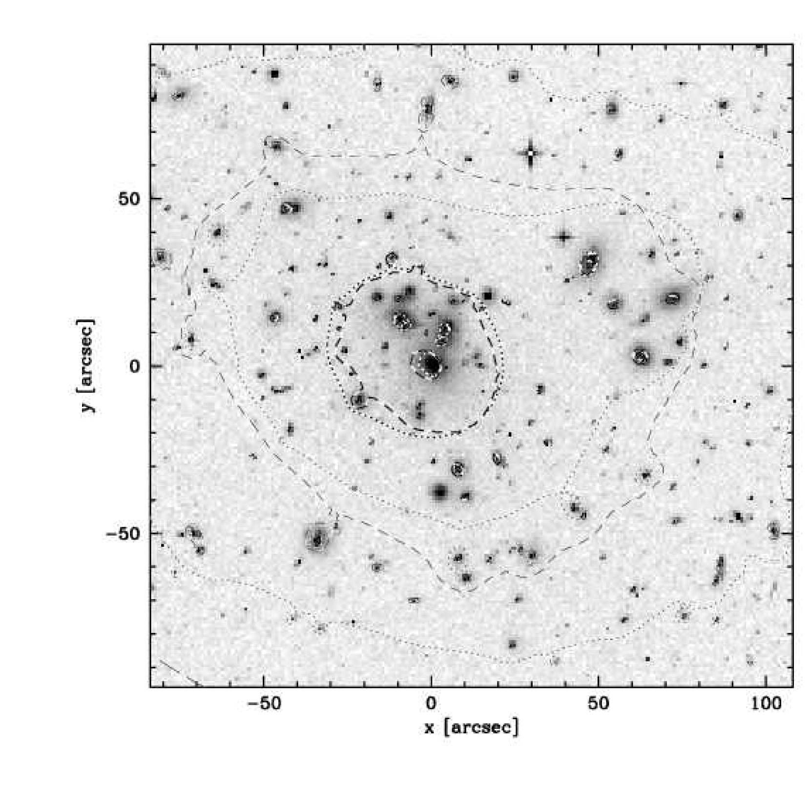
Figure 12: Surface mass density contours for NSIE (dotted) and ENFW (dashed) profiles for Model I. For each smooth DM profile we plot the mean $\kappa$ of the in total 4000 cluster realisations used in deriving the best fit parameters and errors. The contours are drawn at $\kappa$=0.25, 0.50, 1.00 and 2.00 levels for a source at redshift of 1.0. The thin contour lines are for $\kappa<$1 and thick lines for $\kappa\geq$1. The secondary mass concentration on the upper right can also be seen clearly in the surface mass density contours.

Figure 13 shows the critical curves obtained with Models I and II for the two smooth DM profiles. For each smooth DM profile we plot the critical curves of the average cluster of the in total 4000 cluster realisations used in deriving the best fit parameters and errors. The dotted contours are for the NSIE and the dashed contours are for the ENFW profile. The thin contours are drawn for a source redshift of 1 and the thick contours for a source redshift of 5.

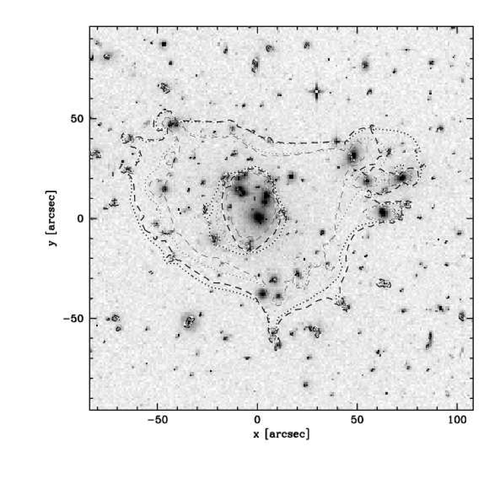
Figure 13: The critical curves obtained with Models I and II for the two smooth DM profiles. For each smooth DM profile we plot the critical curves of the average cluster of the cluster realisations used in deriving the best fit parameters and errors. The dotted contours are for the NSIE and the dashed contours are for the ENFW profile. The thin contours are drawn for a source redshift of 1 and the thick contours for a source redshift of 5.

4.1 Models I and II: Strong Lensing Mass Reconstruction

The first two strong lensing models aim to establish a total mass profile for further analysis. The smooth dark matter component of the cluster mass was modelled in exactly the same way for both models (detailed in section 3), for the galaxy component we vary the scaling of the truncation radius of the BBS model with the velocity dispersion. For Model I we have assumed that the galaxies follow a scaling law similar to the field galaxies, namely that the truncation radius $s$ of a galaxy scales like $s=s_{*}\times(\sigma/136~{}km/s)^{2}$ with the velocity dispersion $\sigma$ of the galaxy. For Model II we have assumed a scaling law expected for galaxies in cluster, $s=s_{*}\times(\sigma/136~{}km/s)$. The normalisation of the scaling law for each Model and smooth DM profile is shown in Table 2. The haloes are strongly truncated. This is a real effect but the actual values obtained for $s_{*}$ can be affected by the optimisation process. Mass lost from galaxies due to truncation can in part be compensated by the smooth dark matter component, leading to possibly significant uncertainties in the truncation radii. It is not our aim in this paper to attempt to constrain the truncation radii of the galaxies in the cluster but instead to reproduce the observed multiple images as accurately as possible. The truncation of galaxies in a cluster environment will be discussed in detail in a forth coming publication (Halkola et al., 2006 in preparation).

The constraints for Models I and II are the positions of the multiple images and their redshifts. The redshifts of sources were allowed to find the optimal redshift within the 1-sigma errors of the photometric redshifts, except sources with spectroscopic redshifts for which we have fixed the redshift to the measured one. The allowed ranges for the source redshifts are tabulated in Table 8 in appendix C.

The best fit parameters for the smooth dark matter component of the models are summarised in Table 2. The errors are caused by errors in determining the correct galaxy masses and in measuring the multiple image position. The derivation of errors is explained in section 4.2.1.

Our best fitting model is Model I with a dark matter component described by an ENFW profile. The differences in the fit quality between the models and smooth dark matter profiles used are generally small as can be seen from Table 2 although both Models perform better when the smooth DM is modelled with an ENFW profile. The fit quality is  0.5” better than that achieved by Broadhurst et al. (2005a) in their analysis of the cluster. This can be due to better modelling of the cluster mass or to a different set of multiple images used. If the difference is due to the changes in multiple image systems then the $\chi^{2}$ in the case Broadhurst et al. (2005a) of is driven by a only a few image systems since most of the images systems are infact identical. Another difference are the constraints imposed on the redshifts of the images in our modelling.

4.2 Models Ib and IIb: Comparison to Broadhurst et al. (2005a)

In order to directly compare the performance of our parametric models to the grid model of Broadhurst et al. (2005a) we have constructed two further models that mimic their setup. The models are constrained only by the multiple image positions from Broadhurst et al. (2005a); the photometric redshifts of the images were thus ignored and were included as free parameters. We have fixed the spectroscopic redshifts however since it is necessary to define an overall mass scale for the cluster. The rest of the modelling is identical to that of Models I and II.

The very good performance of our models relative to Broadhurst et al. (2005a) is remarkable considering the large freedom in the mass profile allowed in their modelling. This also means that the mass profile can be very well described by parametric models making the additional freedom allowed by non-parametric mass modelling unnecessary, even undesirable if one is interested in comparing the performance of different parametric mass profiles.

Assuming that the smooth mass component of Broadhurst et al. (2005a) is able to reproduce both NSIE and ENFW halo profiles the other major difference between our mass modelling and that of Broadhurst et al. (2005a) is in the treatment of the galaxy component. The assumptions needed on the properties of the cluster galaxies in our modelling seem to be well justified based on the superior performance of our models.

4.2.1 Estimation of Errors in the Parameters of the Smooth Dark Matter Component

Our primary source of uncertainty in the parameters of the smooth dark matter component are the velocity dispersions of the galaxies in the cluster.

In order to estimate the effect of measurement errors in the cluster galaxy component on the parameters of the smooth cluster component we have created 2000 clusters for Models I, II, Ib and IIb and the two profiles by varying the velocity dispersions of cluster galaxies and positions of multiple images by the estimated measurement errors. For each galaxy we have assigned a new velocity dispersion from a Gaussian distribution centred on the measured values with a spread corresponding to the error. The truncation radii of the cluster galaxies were adjusted accordingly. For the scaling law we have used the normalisation as for the original cluster galaxies. New positions for the multiple images were assigned similarly by assigning new positions from a Gaussian distribution centred on the measured positions.

Optimal parameters for the smooth cluster component for each cluster were found by minimising $\widetilde{\chi}^{2}$ in the source plane due to the large number of minimisations required. However, in all subsequent analysis we have used the image plane $\chi^{2}$ calculated after the optimal parameters in the source plane were found.

To justify the use of $\widetilde{\chi}^{2}$ instead of $\chi^{2}$ in the error estimation we show in Figure 14 the final $\chi^{2}$ against $\widetilde{\chi}^{2}$ for a large number of models after minimising $\widetilde{\chi}^{2}$. In the figure both $\chi^{2}$ and $\widetilde{\chi}^{2}$ have been scaled by the minimum $\widetilde{\chi}^{2}$ of the models. The good correspondence between the two, even at high values of $\chi^{2}$, and that $\chi^{2}(\widetilde{\chi}^{2})$ is a monotonically increasing function (unfortunately with some scatter) gives us confidence in the source plane minimisation and our error analysis.

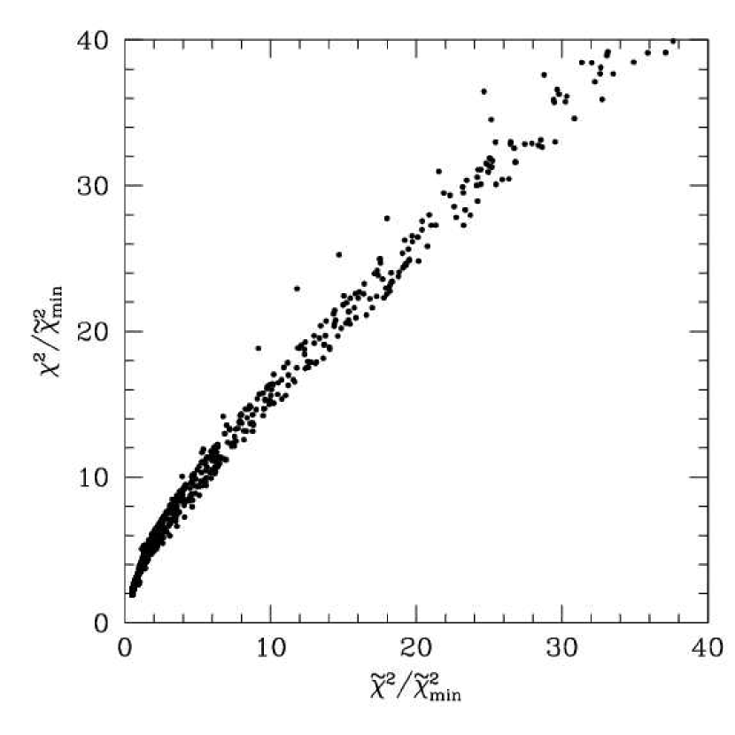
Figure 14: A comparison between $\chi^{2}$ (image plane $\chi^{2}$) and $\widetilde{\chi}^{2}$ (source plane $\chi^{2}$) for $\sim$3000 different model configurations. The important property of $\chi^{2}(\widetilde{\chi}^{2})$ for the minimisation is that it is a monotonically increasing function making $\widetilde{\chi}^{2}$ a reliable tracer for $\chi^{2}$ when used in finding optimal model parameters in the error analysis.

The optimal parameters of the generated clusters have a spread around the best fit parameters determined for the ’real’ cluster. The number density of the optimal parameters in the parameter space cannot be directly used to quantify the random error since areas of high density could in fact also include a large number of relatively poor fits to the data. To include also information of the quality of fit we weight each realisation of the Monte-Carlo simulation with the final 1/$\chi^{2}$ of the realisation. In Figure 15 we show the number density contours for the NSIE (top panel) and ENFW (bottom panel) halo parameters of the realisations after weighting by the final 1/$\chi^{2}$. The solid lines are for Model I and the dashed lines for Model II. The contour lines show the regions in which 68% and 95% of the weighted realisations lie.

Figure 15: Estimates of the profile parameter uncertainties for the main halo of the smooth DM component (NSIE top, NFW bottom). In both panels Model I is represented by the solid contours and Model II by the dashed contours. Contours are drawn at 68% and 95% confidence levels. The uncertainty is mostly due the errors in determining the contribution of the cluster galaxies to the total mass.

Table 2: Best fit halo parameters of the smooth dark matter components for Models I and II. The rms error quoted for each model and halo type is the rms distance between the measured image positions and those predicted by the models expect for image systems where the calculations of an image plane $\chi^{2}$ was not possible (8, 12, 14, 15, 30, 31 and 32) for which we have used the source plane $\chi^{2}$ defined in equation 6. The values given are for the best fitting halo optimised in the image plane. The values in brackets refer to the mean values obtained from the simulations (optimised in the source plane), the errors in the halo parameters are derived from the spread of the values in the simulations. For details of the models and error derivation see text body.

	Model I		Model II
NSIE	rms error 3.17”  (3.51$\pm$0.15”)		rms error 3.13”  (3.45$\pm$0.16”)
	sbbs = 24 kpc*$(\sigma_{gal}$/136km/s)2		sbbs = 37 kpc*$(\sigma_{gal}$/136km/s)
Parameter	Halo One	Halo Two	Halo One	Halo Two
$\sigma$ (km/s)	1298  (1293${}^{+11}_{-10}$)	603  (595$\pm$20)	1285  (1281${}^{+10}_{-9}$)	618  (613$\pm$17)
rc (kpc)	77  (76${}^{+4}_{-3}$)	75 kpc  (72$\pm$5)	75  (74${}^{+3}_{-3}$)	75 kpc  (73$\pm$4)
ENFW	rms error 2.73”  (3.12$\pm$0.20”)		rms error 2.48”  (3.08$\pm$0.19”)
	sbbs = 21 kpc*$(\sigma_{gal}$/136km/s)2		sbbs = 36 kpc*$(\sigma_{gal}$/136km/s)
Parameter	Halo One	Halo Two	Halo One	Halo Two
C	6.5  (6.3$\pm$0.2)	0.5  (0.5$\pm$0.1)	6.2  (6.2$\pm$0.1)	0.7  (0.7$\pm$0.1)
r200 (Mpc)	2.04  (2.03$\pm$0.03)	2.79  (2.81$\pm$0.06)	2.07  (2.06$\pm$0.03)	2.52  (2.53$\pm$0.06)
Model free parameters	parameters of the smooth dark matter component		parameters of the smooth dark matter component
Model constraints	images from this work and Broadhurst et al. (2005a) zphot of sources		images from this work and Broadhurst et al. (2005a) zphot of sources

Table 3: Best fit halo parameters of the smooth dark matter components for Models Ib and IIb. The rms error quoted for each model and halo type is the rms distance between the measured image positions and those predicted by the models expect for image systems where the calculations of an image plane $\chi^{2}$ was not possible (8, 12, 13, 14, 20 and 30) for which we have used the source plane $\chi^{2}$ defined in equation 6. The values given are for the best fitting halo optimised in the image plane. The values in brackets refer to the mean values obtained from the simulations (optimised in the source plane), the errors in the halo parameters are derived from the spread of the values in the simulations. For details of the models and error derivation see text body.

	Model Ib		Model IIb
NSIE	rms error 3.03”  (3.27$\pm$0.20”)		rms error 2.65”  (3.29$\pm$0.21”)
	sbbs = 30 kpc*$(\sigma_{gal}$/136km/s)2		sbbs = 43 kpc*$(\sigma_{gal}$/136km/s)
Parameter	Halo One	Halo Two	Halo One	Halo Two
$\sigma$ (km/s)	1223  (1222$\pm$13)	647  (645$\pm$18)	1210  (1216$\pm$11)	658  (660$\pm$15)
rc (kpc)	56  (60$\pm$3)	75  (74$\pm$3)	58  (60$\pm$3)	74  (74$\pm$2)
ENFW	rms error 2.74”  (3.30$\pm$0.15”)		rms error 2.72”  (3.31$\pm$0.15”)
	sbbs = 31 kpc*$(\sigma_{gal}$/136km/s)2		sbbs = 51 kpc*$(\sigma_{gal}$/136km/s)
Parameter	Halo One	Halo Two	Halo One	Halo Two
C	6.4  (6.4$\pm$0.2)	1.5  (1.6$\pm$0.1)	6.5  (6.4$\pm$0.2)	1.6  (1.7$\pm$0.1)
r200 (Mpc)	2.12  (2.08$\pm$0.04)	1.87  (1.86$\pm$0.05)	2.08  (2.04$\pm$0.04)	1.85  (1.83$\pm$0.05)
Model free parameters	parameters of the smooth dark matter component, zphot of sources		parameters of the smooth dark matter component, zphot of sources
Model constraints	images from Broadhurst et al. (2005a)		images from Broadhurst et al. (2005a)

Table 4: Best fit halo parameters for the cluster profile. For Models III and IV we have fitted the measured cluster parameters with a single NSIS or NFW profile. The constraints for the cluster parameters were mass for Model III,both mass and shear for Model IV. For details of the models see text body.

	Model III	Model IV
NSIE	$\chi^{2}$ / dof = 10.5 / 11	$\chi^{2}$ / dof = 30.0 / 20
Parameter	only one halo fitted	only one halo fitted
$\sigma$	1514${}^{+18}_{-17}$ km/s	1499${}^{+15}_{-14}$ km/s
rc	71$\pm$5 kpc	66$\pm$5 kpc
ENFW	$\chi^{2}$ / dof = 0.8 / 11	$\chi^{2}$ / dof = 31.9 / 20
Parameter	only one halo fitted	only one halo fitted
C	6.0$\pm$.5	7.6${}^{+0.3}_{-0.5}$
r200	2.82${}^{+0.11}_{-0.09}$ Mpc	2.55${}^{+0.07}_{-0.04}$ Mpc
Model free parameters	the above parameters of the halo profiles	the above parameters of the halo profiles
Model constraints	total mass obtained with Models I and II	total mass obtained with Models I and II shear from Broadhurst et al. 2005b

4.3 Model III: Parameters for the Total Mass Profile

It is important to realise that the multiple images constrain the combined mass of the cluster, be it baryonic or dark. The division of the mass to two components is done in order to take account of the mass we can observe as accurately as possible. The uncertainty of the description of the galaxy component is reflected in how well we can determine the profile parameters of the smooth dark matter component. The parameters for the total mass distribution, constrained directly by the multiple images, can be determined significantly better. For this reason we have also fitted single NFW and NSIS haloes to the total mass obtained from Models I and II.

We estimate the total mass profile of the cluster by combining all mass profiles from the error analysis. In Figure 16 we show the 68.3% confidence regions of mass for the two mass components and the total mass. The galaxy component is shown as a solid grey region, smooth dark matter as a striped grey and the total mass as a solid black region. The regions were determined by taking the best 68.3% of the galaxy component realisations from both Models I and II regardless of the smooth DM profile used. We have decided to combine the individual mass profiles from both models and smooth dark matter profiles since they all provide similar fit qualities and by combining them we allow a greater freedom in the total mass profile.

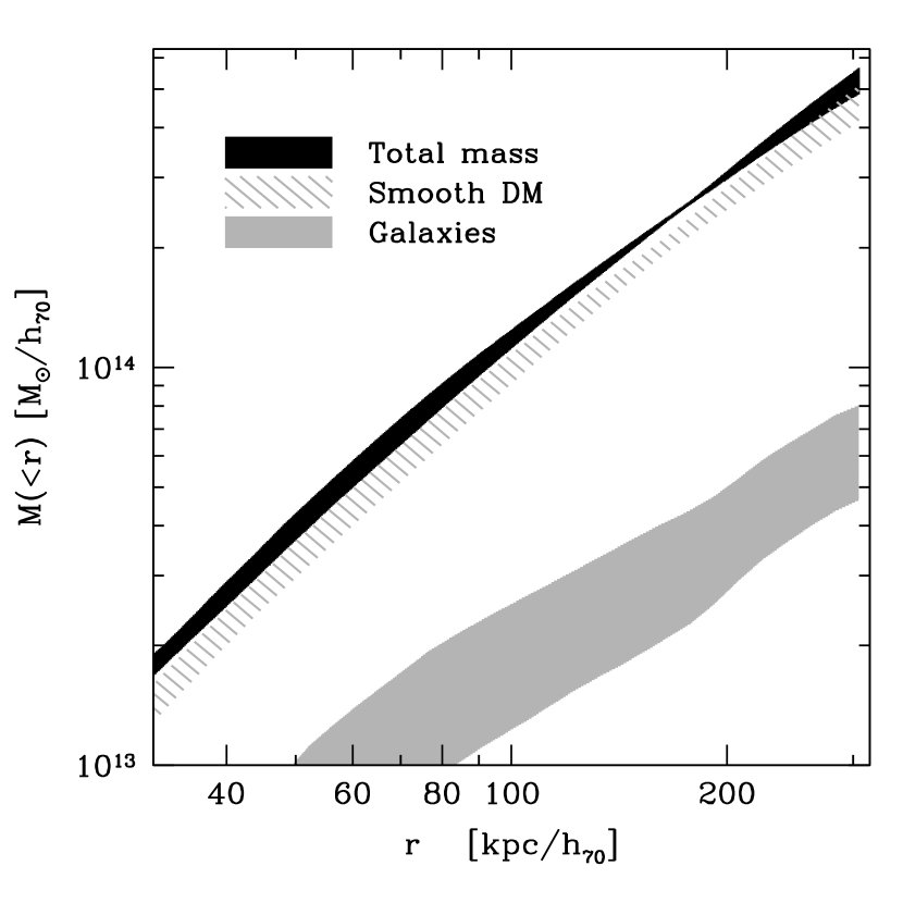
Figure 16: 1-$\sigma$ confidence regions of projected mass M($<$r) inside radius r for two mass components and total mass. The mass associated with galaxies is shown as a solid grey, the smooth dark matter as a striped grey and the total mass as a solid black region. The large uncertainty in the galaxy component is well balanced by the smooth dark matter component to produce a tight M($<$r) profile for the total mass.

In Figure 17 we show again the envelope of the total masses encompassed by the best 68.3% fits of all the model galaxies from the error analysis in striped grey. For comparison we also show the strong lensing mass measurement of Broadhurst et al. (2005a) (long dashed), weak lensing mass from King et al. (2002) (NFW dashed, SIS dot dashed) and X-ray mass estimate of Andersson & Madejski (2004) (dashed - long dashed). For Broadhurst et al. (2005a) and Andersson & Madejski (2004) points we plot the 1-sigma errors. The Broadhurst et al. (2005a) mass has been integrated from the radial surface mass density profile in their Figure 26, and the errors have been inferred from the errors in surface mass density. Andersson & Madejski (2004) have also provided an estimate of the projected X-ray mass so that the profile can be compared with lensing mass measurements. The agreement between our work and that of Broadhurst et al. (2005a) is very good, well within 1-$\sigma$ at all radii. The mass measured using strong lensing is factor $\sim$2 larger than the mass from X-ray estimates. For a discussion on the low mass from X-ray please refer to Andersson & Madejski (2004).

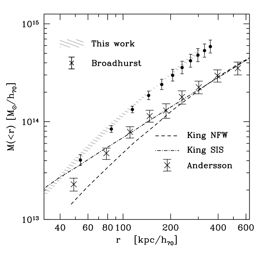
Figure 17: 1-$\sigma$ confidence region of projected mass M($<$r) inside radius r from this work (striped grey region) compared with Broadhurst et al. (2005a) (long dashed), King et al. (2002) (NFW dashed, SIS dot dashed) and Andersson & Madejski (2004) (dashed - long dashed). The error bars shown for Broadhurst et al. (2005a) and Andersson & Madejski (2004) are 1-$\sigma$ errors. The mass profile and errors for Broadhurst et al. (2005a) were obtained by integration from the surface mass density in their Figure 26.

To estimate the NSIS and NFW parameters of the total mass we can simply fit the mass profile obtained with Models I and II with a single NSIS or NFW halo. One should not forget that the total mass profile was derived using the NSIE and NFW profiles themselves. The total mass profile is composed of the mass in the galaxies and two elliptical smooth DM haloes and hence the total mass is no longer a pure NSIE or ENFW profile. In fitting a single halo we also do not include ellipticity. The excellent agreement between the total mass profile obtained in this work and that of Broadhurst et al. (2005a) and the superior performance of our models to theirs give us confidence that the parameters we have derived are indeed representative of the total mass profile of the cluster. We do not compare the quality of fit of NSIS and NFW haloes but instead the obtained parameters with those from weak lensing. This should help us to avoid problems arising from the underlying smooth DM profiles used in obtaining the total mass profile.

The 68.3%, 95.4% and 99.7% confidence contours for the NFW parameters are shown in Figure 20 (solid black contours). Both the concentration and r₂₀₀ are well constrained. The best fit values are C=6.0$\pm$0.5 and r₂₀₀=$2.82^{+0.11}_{-0.09}$.

Also the NSIS parameters are well constrained. The corresponding confidence contours are shown in Figure 21. Both of the NSIS parameters depend on the halo profile in the region where the multiple images have significant constraints. Therefore the confidence contours are also extremely tight. The best fit parameters are $\sigma$=1514${}_{-17}^{+18}$ km/s and $r_{c}$=71$\pm$5 kpc. The best fitting profile parameters are summarised in Table 4.

As a comparison we have also fitted of a single isothermal sphere to the smooth DM component only. This results in an NSIS a velocity dispersion of 1450${}^{+39}_{-31}$ km/s and a core radius of 77${}^{+10}_{-8}$ kpc/h while an NFW profile has a concentration of 4.7${}^{+0.6}_{-0.5}$ and a virial radius of 2.86$\pm$0.16 Mpc/h₇₀.

4.4 Model IV: Combining Information from Strong and Weak Lensing

In this subsection we include the new weak lensing shear data from Broadhurst et al. (2005b) in our analysis to use information of the cluster profile from larger clustercentric radii.

Strong lensing in A1689 can only constrain the mass at best to out 200-300 kpc from the cluster centre. In order to constrain the scale radius of an NFW profile strongly it should lay within the multiple images. Unfortunately, in the case of A1689, the scale radius seems to be just outside the multiple images (and hence strong lensing cannot constrain it significantly) but too small to be well constrained by weak lensing data alone. On the other hand weak lensing can tell us something about the total mass of the cluster and hence constrain r₂₀₀. By combining this with information from strong lensing (details of the profile at small radii) one should expect to have a handle on the cluster at all radii.

In their extensive work on this cluster Broadhurst et al. (2005a, b) conclude that the parameters derived from strong and weak lensing are not compatible. In the strong lensing regime an NFW halo has only a moderate concentration (C=6.0$\pm$0.5 in this work, Broadhurst et al. (2005a) find C=6.5${}^{+1.9}_{-1.6}$) whereas in the weak lensing regime a very high concentration (Broadhurst et al. (2005b) C=13.7${}^{+1.4}_{-1.1}$) is required, uncharacteristic to a halo of this size and typical to a halo with a much lower mass.

We have checked this inconsistency in the NFW parameters by fitting a single halo to both the radial mass profile (Model III, this work) and shear profile (Broadhurst et al. (2005b)), shown in Figures 18 and 19. The fit is done simultaneously to the mass from strong lensing and reduced shear from weak lensing. The best fitting NFW profile is plotted as a dashed black line in the two figures.

Figure 18: Radial profile of the total mass from this work (circles). The lines show the best fitting NSIS (solid line) and NFW (dashed line) profiles to a simultaneous fit of the shear in Figure 19 and the mass in this Figure.

Figure 19: Radial profile of the tangential shear from Broadhurst et al. (2005b) (circles). The lines show the best fitting NSIS (solid line) and NFW (dashed line) profiles to a simultaneous fit of the shear in this figure and the mass in Figure 18.

Unlike Broadhurst et al. (2005b) we do not include any prior (C$\leq$30) on the concentration in our fits since there is no obvious bias towards NFW profiles with higher concentrations: a high quality fit with a large concentration purely reflects the inability of shear measurements to constrain the central cluster profile. A prior could lead to a wrong determination of the minimum $\chi^{2}$ and hence favour a smaller concentration without a physical significance.

Fitting a single NFW halo to the weak lensing shear from Broadhurst et al. (2005b) gives only a lower limit for the concentration but constrains r₂₀₀ (or equivalently virial mass M₂₀₀) to $\sim$ 2.0-2.5Mpc/h₇₀ (68.3%, 95.4% and 99.7% confidence regions for C-r_s are shown in Figure 20 as dotted lines). The best fit values are C=30.4 and r₂₀₀=1.98 Mpc/h₇₀. The fit is excellent with $\chi^{2}_{WLshear}/dof$ = 2.5 / 8. The parameters of the NFW profile from fitting the total mass and shear independently disagree more than the estimated 3-$\sigma$ errors.

By fitting both shear and mass simultaneously we are able to combine the constraints from both small and large radii to obtain well defined NFW parameters for the halo. The NFW parameters in this case become C=7.6${}^{+0.3}_{-0.5}$ and r₂₀₀=2.55${}^{+0.07}_{-0.09}$ Mpc/h₇₀ (confidence regions for the combined weak and strong lensing fit are shown with solid red contours in Fig. 20). The mass and shear profiles of the best fitting NFW halo are shown in Figures 18 and 19 respectively as dashed lines.

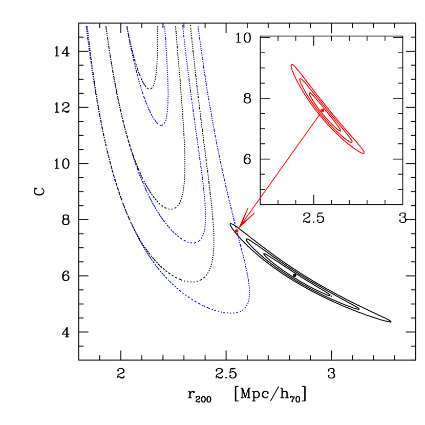
Figure 20: 68.3%, 95.4% and 99.7% confidence contours for the NFW parameters C-r₂₀₀ for a fit to reduced shear (data from Broadhurst et al. (2005b)) only (dotted contours) and mass (data from this work) only (solid black contours). The dotted blue contours show the confidence regions from shear when the last two data points are excluded. The combined fit to both reduced shear and mass simultaneously is $\chi^{2}/dof\sim$ 31.9 / 20 (shown in the inlet for clarity with the same scale). The best fitting parameters are C=7.6${}^{+0.3}_{-0.5}$ and r₂₀₀=2.55${}^{+0.07}_{-0.09}$ Mpc/h₇₀. A fit to shear only gives C=30.4 and r₂₀₀=1.98 Mpc/h₇₀.

We have repeated the experiment also for an NSIS halo. The corresponding contours are shown in Figure 21, and mass and shear profiles in Figures 18 and 19 as solid lines.

Like with the NFW halo the core radius of the NSIS halo is poorly constrained by the weak lensing data alone though surprisingly a singular profile with $\sigma$=1354 km/s has the best fit. The fit is good with $\chi^{2}$ / dof = 10 / 8. The best fitting parameters to both weak and strong lensing simultaneously are $\sigma$=1499$\pm$15 km/s and r_c=66$\pm$5 kpc/h₇₀ with $\chi^{2}$ / dof = 30 / 20. The agreement between the parameters for the NSIS halo is better than for the NFW profile, though still only at 2-$\sigma$ level.

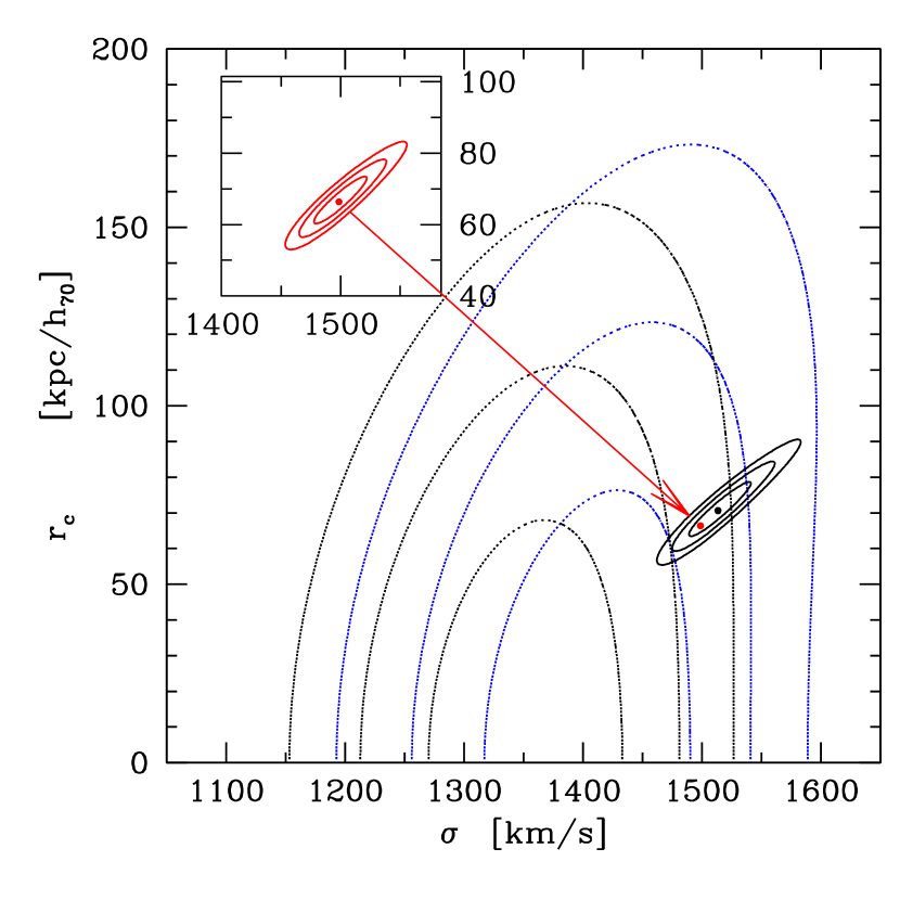
Figure 21: 68.3%, 95.4% and 99.7% confidence contours for the NSIS parameters $\sigma$-r_c for a fit to reduced shear (data from Broadhurst et al. (2005b)) only (dotted contours) and mass (data from this work) only (solid black contours). The dotted blue contours show the confidence regions from shear when the last two data points are excluded. The combined fit to both reduced shear and mass simultaneously (shown in the inlet with the same scale) is similar to that of NFW profile with $\chi^{2}/dof\sim$ 30 / 27. The best fitting parameters are $\sigma$=1499$\pm$15 km/s and r_c=66$\pm$5 kpc/h₇₀.A fit to shear only gives a singular profile with $\sigma$=1354 km/s.

To see how important the last two shear data points are for the previously derived cluster parameters we have excluded the two outer most data points from the shear measurement. If compared to numerical simulations the concentration of the NFW halo remains unreasonably high although the disagreement between weak and strong lensing is reduced to just under 3-sigma. For the NSIS halo the shear data is still fit best with a singular profile but higher values of core radius are allowed and the velocity dispersion is increased to make the weak and strong lensing parameters agree at better than 2-sigma. The best fitting parameters are C=7.1$\pm$0.4 and r₂₀₀=2.63$\pm$0.06 Mpc/h₇₀ for the NFW halo and $\sigma$=1505$\pm$15 km/s and r_c=68$\pm$5 kpc/h₇₀ for the NSIS halo. The two profiles fit well with $\chi_{nsis}^{2}/dof\sim$ 22 / 18 compared to $\chi_{nfw}^{2}/dof\sim$ 20 / 18. The confidence regions with the last two shear points excluded are shown as dotted blue contours in Figures 20 and 21.

In a recent work Biviano & Salucci (2005) derived the mass profiles of the different luminous and dark components of cluster masses separately. They find that ratio of baryonic to total mass decreases from the centre to r$\sim$0.15 virial radii and then increases again. We see the same trend also in our work (Figure 16), where the galaxy component has a minimum contribution at around 200 kpc. This is smaller than expected (380 kpc) if we take the r₂₀₀ of the NFW profile to be the virial radius of the cluster.

The best fit parameters are summarised in Table 4.

4.5 Comparison with Literature

The mass of Abell 1689 has been determined in a variety of ways with different weaknesses and strengths. Results from the three methods used (X-ray temperature, line-of-sight velocity and lensing (both weak and strong)) have disagreed considerably. This section makes a short summary and comparison of the results using the different methods.

Recent results are summarised in Tables 5 and 6. Parametric model fits are summarised in Table 5 and aperture mass fits in Table 6. When comparing different mass estimates one should bear in mind that both X-ray and velocity dispersion measure a spherical mass where as lensing in the thin lens approximation measures projected mass, i.e. mass in a cylinder of a given radius, resulting in higher masses within a given radius. Only lensing measures the mass directly. Both X-ray and velocity dispersion rely on the cluster being a relaxed system.

Table 5: Comparison between best fit parametric mass models from different methods for Abell 1689. Andersson & Madejski (2004) is an X-ray, King et al. (2002) a weak lensing and Girardi et al. (1997) a line of sight velocity study of the cluster. The background galaxy catalogue used by King et al. (2002) suffers from contamination from galaxies at low redshifts where lensing is inefficient (discussed in more detail in Clowe & Schneider (2001)) which reduce the total measured mass of the cluster and hence the measured velocity dispersion.

	NFW Parameters
Method	C	r200 (Mpc)	Reference
SL	6.0$\pm$0.5	2.82$\pm$0.11	this work
SL	6.5${}^{+1.9}_{-1.6}$	2.02	Broadhurst et al. 2005a
X-ray	7.7${}^{+1.7}_{-2.6}$	1.87$\pm$0.36	Andersson & Madejski 2004
WL	4.8	1.84	King et al. 2002
	NSIE Parameters
Method	$\sigma$ (km/s)	rc (kpc)	Reference
SL	1514$\pm$18	71$\pm$5	this work
SL	1390	60	Broadhurst et al. 2005a
X-ray	918$\pm$27	SIS	Andersson & Madejski 2004
X-ray	1190	27	Andersson & Madejski 2004∗
WL	998${}^{+33}_{-42}$	SIS	King et al. 2002
LOSVD	1429${}^{+145}_{-96}$	-	Girardi et al. 1997
∗ data from Andersson & Madejski 2004, fitting done in this work.

Table 6: Comparison between mass estimates for Abell 1689 from different methods. The mass measured by Andersson & Madejski (2004) are underestimates of the total mass if the cluster is undergoing a merger. For our work the mass at r=0.25 Mpc/h₇₀ is an extrapolation since the multiple images do not extend to such large clustercentric radii.

M($<$r)	r	Reference
(1015 M⊙ h${}_{100}^{-1}$)	(Mpc h${}_{100}^{-1}$)
0.14 $\pm$ 0.01	0.10	this work, Model III
0.082 $\pm$ 0.013	0.10	Andersson & Madejski (2004)
0.43 $\pm$ 0.02	0.24	Tyson & Fischer (1995)
0.20 $\pm$ 0.03	0.25	Andersson & Madejski (2004)
0.37 $\pm$ 0.06	0.25	this work, Model III
0.48 $\pm$ 0.16	0.25	Dye et al. (2001)

4.5.1 X-ray

The most recent X-ray measurements of the mass of A1689 are those of Xue & Wu (2002) with the Chandra X-Ray Observatory and Andersson & Madejski (2004) with the XMM-Newton X-Ray Observatory. Both find nearly circular X-ray emission centred on the cD galaxy. Best fit NFW profile to Andersson & Madejski (2004) data has parameters $c=$7.7${}^{+1.7}_{-2.6}$ and $r_{200}=$$\pm$0.36 Mpc/h₇₀. They have also fitted a SIS profile to the data and obtain $\sigma=$918 km/s. The NFW profile gives a much better fit to their data. We have also fitted an NSIS profile to Andersson & Madejski (2004) since it is clear that (single parameter) a SIS will not be able to reproduce the data. We have fitted the spherical mass of an NSIS profile with $\sigma=$1190 km/s and $r_{c}=$27 kpc to the data from Figure 9 of Andersson & Madejski (2004) and this provides a very good fit. The NSIS halo along with the fitted points are shown in Figure 22. The low $\sigma$ found by Andersson & Madejski (2004) is mainly driven by the low central mass of the cluster which the SIS profile can only accommodate with a low $\sigma$. By including a core radius in the fit the mass can be modelled very well everywhere also by an IS profile.

Figure 22: The spherical mass of A1689 from X-ray observations of the cluster by Andersson & Madejski (2004) (points) and our best fit NSIS halo with $\sigma$=1190 km/s and $r_{c}=$27 kpc (line). The fit is very good with $\chi^{2}$ / dof = 9.2 / 8. The low mass in the centre can only be fitted with an isothermal sphere if a core radius is included.

The total mass inside 140kpc from the cluster centre is 1.2$\times$10¹⁴ M_⊙ and 1.9$\times$10¹⁴ M_⊙ for Andersson & Madejski (2004) and Xue & Wu (2002) respectively. Andersson & Madejski (2004) also discuss the effect a merger would have on the X-ray mass estimates. The estimated X-ray masses could increase by a factor of $\sim$2 (velocity dispersion by factor $\sqrt{2}$) assuming that two equal mass haloes are considered as one in the X-ray analysis. This would be enough to bring X-ray mass of Abell 1689 in good agreement with lensing.

4.5.2 Spectroscopy

An early spectroscopic work by Teague et al. (1990) found a very high velocity dispersion of 2355km/s for Abell 1689. Girardi et al. (1997) have reanalysed the data from Teague et al. (1990) and found four different structures in A1689 with velocity dispersions of 1429km/s, 321km/s, 243km/s and 390km/s. A simple consideration of total mass in the separate structures equals that of a single isothermal sphere with $\sigma$$\sim$1550km/s. The separate structures are more extended than the region of multiple images and the 2^nd halo in this study does not correspond to any of the spectroscopically identified groups by Girardi et al. (1997).

Czoske (2004) have used VIMOS on the VLT to obtain spectra for A1689. Their results are still preliminary but indicate a strong gradient in the velocity dispersion from $\sim$2100km/s in the centre to $\sim$1200km/s at larger clustercentric distances ($\gtrsim$1Mpc). The high velocity dispersion on the centre could be due to an unrelaxed system and not an indication of a high total mass of the cluster.

Lokas et al. (2005) have recently shown that cluster mass cannot be reliably estimated from galaxy kinematics due to the complex kinematical structure of A1689. The obtained velocity dispersion depends sensitively on the chosen galaxy sample.

4.5.3 Weak Lensing

The mass of A1689 has been measured in a number of cases with weak gravitational lensing. The obtained masses are always considerably lower when compared to strong lensing masses or LOSVD measurements with $\sigma$=1028 km/s, $\sigma$=998 km/s and $\sigma$=1030 km/s (Clowe & Schneider (2001), King et al. (2002a,b) respectively). Clowe & Schneider (2001); King et al. (2002) use the same catalogue of lensed background galaxies. The catalogue is very likely contaminated by unlensed galaxies in the foreground and only weakly lensed galaxies in the close proximity of the cluster ($z<$0.3) where lensing is inefficient. These galaxies reduce the average shear signal leading to lower mass estimates. The SIS velocity dispersion estimate of Clowe & Schneider (2001) increases to 1095 km/s if they assume that 87% of the faint background galaxies have $z>$0.3. Recent work by Broadhurst et al. (2005b) results in higher masses and only 1-2 $\sigma$ discrepancy between weak and (our) strong lensing models.

Hoekstra (2003) investigate the effect of distant (along line-of-sight) large scale structure on the errors of derived M₂₀₀ and concentration of an NFW halo. They conclude that the errors could be underestimated by a factor $\sim$2.

5 Conclusion

We have identified 15 images systems in deep ACS images of galaxy cluster Abell 1689. Two of these are not in the 30 image systems identified by Broadhurst et al. (2005a). By excluding one of their image systems and splitting another in two we have constructed a new catalogue with 107 multiple images. These from 31 image systems and we have additionally used one long arc in the modelling. The galaxy cluster was modelled with a two component mass model: mass associated with cluster galaxies and an underlying smooth dark matter component. Cluster galaxies were identified from the cluster redsequence and their halo masses were estimated using Fundamental-Plane and Faber-Jackson relations. The use of Fundamental-Plane in measuring the mass for most of the galaxies used in the cluster modelling is new and allows a very precise determination of the (central) galaxy mass. The galaxies were modelled with a truncated isothermal ellipsoid. The truncation of the galaxy haloes is necessary for accurate lensing models. The smooth dark matter component was modelled separately with two parametric elliptical halo profiles: elliptical NFW profile and a non-singular isothermal ellipsoid.

We find that both an ENFW and NSIE describe the smooth dark matter component very well. The multiple images are reproduced extremely well. The best fit ENFW profile of the smooth dark matter component has a virial radius of 2.06$\pm$0.03 Mpc and a concentration parameter of 6.2$\pm$0.1, the best fitting NSIE profile has a core radius of 74$\pm$3 kpc and a velocity dispersion of 1281$\pm$10 km/s. The ellipticities of the two model haloes are small ($\epsilon=0.06$ in both cases).

By fitting a single NSIS and NFW halo to the total mass we can determine the halo parameters of the cluster as a whole very strongly. The NFW parameters are C=6.0$\pm$0.5 and r₂₀₀=2.82$\pm$0.11 Mpc; the NSIS parameters are $\sigma$=1514${}_{-17}^{+18}$ km/s and $r_{c}$=71$\pm$5 kpc.

Using the images of Broadhurst et al. (2005a) we obtain a fit with an rms distance between the identified multiple images and model predictions 0.6” better than the best model in Broadhurst et al. (2005a) (rms of 2.65” compared to 3.25”). This is surprising considering the large freedom in the mass model used by Broadhurst et al. (2005a) compared to parametric models. The superior performance of our model can in part be attributed to a careful analysis of the cluster galaxy component. It also indicates that small scale dark matter ’mini’ haloes are not needed to explain the deflection field in A1689. The overall mass profiles are in good agreement however. This shows that strong gravitational lensing can be used to derive very accurate total mass profiles; different methods and assumptions agree very well in mass although the treatment of the cluster galaxies in particular can be quite different.

The low masses obtained from weak lensing in the past are no longer observed in new shear measurements by Broadhurst et al. (2005b). According to our analysis, at least for the NFW profile, the parameters obtained from strong and weak lensing disagree at $\sim$3-sigma level. The high concentration of an NFW profile fit to weak lensing data is incompatible with both the strong lensing results presented here and in Broadhurst et al. (2005a). The discrepancy between halo parameters is present at $<$2-sigma level in the case of an isothermal sphere dark matter halo. We do not find support for the strong rejection of a softened isothermal sphere by Broadhurst et al. (2005b) based on the combined strong and weak lensing mass profile.

The unusually high concentration (compared to numerical N-body simulations) can be explained by a suitably aligned tri-axial halo (Oguri et al., 2005) but this cannot be used to solve the discrepancy between weak and strong lensing measurements which both measure the same projected mass, albeit at different radii.

Appendix A Gravitational Lensing by NSIE, NFW and BBS profiles

A.1 Isothermal Sphere / Ellipsoid

A model often used in gravitational lensing for galaxies and clusters of galaxies is a singular isothermal sphere (SIS) (e.g. Gott & Gunn, 1974; Turner et al., 1984). SIS naturally reproduces the observed flat rotation curves of galaxies (e.g. Roberts & Rots, 1973). The following equations describe a non-singular (or softened) isothermal ellipsoid (Hinshaw & Krauss, 1987) where the singularity has been removed with a core radius, and additionally an ellipticity has been incorporated to better model the observed galaxy shapes (Seitz et al., 1998). In the equations ellipticity is introduced to the gravitational potential, in a similar fashion to Kochanek et al. (1989), and not the mass distribution. This approach has some problems with large ellipticities, when the accompanying mass distribution can have negative values, as noted by Blandford & Kochanek (1987), Kormann et al. (1994) and others, but is numerically rather simple and straightforward to implement since all parameters of interest can be calculated from the analytic derivatives of the potential. An alternative approach is to have an elliptical mass distribution as demonstrated by Kormann et al. (1994) but the expressions for deflection angle ($\vec{\alpha}$), surface mass density ($\kappa$) and shear ($\vec{\gamma}$) are considerably more complicated. Kassiola & Kovner (1993) have done a thorough comparison between elliptical potentials and elliptical mass distributions. We have estimated the effect of an elliptical potential on the ellipticity of the surface mass density, illustrated in Figure 6. This will be discussed later in more detail.

In the following equations $\psi$ is gravitational potential, $\vec{\theta}$ is (image) position on the lens plane, $\zeta$ is a core radius, $q$=b/a=(1-$\epsilon$)/(1+$\epsilon$) is the axis ratio of the potential and $\theta_{E}$ is the Einstein radius of a singular isothermal sphere.

The equations for the deflection potential ($\psi(\vec{\theta})$), the deflection angle ($\vec{\alpha}$), $\kappa$ and $\vec{\gamma}$ are

$$\psi(\vec{\theta})={\psi_{0}\over\zeta}\ \sqrt{\zeta^{2}+q\ \theta_{1}^{2}+{1\over q}\ \theta_{2}^{2}}=\theta_{E}\ C(\vec{\theta})\ ,$$ (7)

with $\theta_{E}={\psi_{0}\over\zeta}=4\pi{D_{ds}\over D_{s}}({\sigma\over c})^{2}$ and $C(\vec{\theta})=\sqrt{\zeta^{2}+q\ \theta_{1}^{2}+{1\over q}\ \theta_{2}^{2}}$ ,

$$\vec{\alpha}(\vec{\theta})=\nabla\psi(\vec{\theta})={\theta_{E}\over C(\vec{\theta})}\cdot\bigg{(}q\ \theta_{1},\ {1\over q}\ \theta_{2}\bigg{)}\ ,$$ (8)

$$\kappa(\vec{\theta})={1\over 2}\nabla^{2}\psi(\vec{\theta})={1\over 2}\ {\theta_{E}\over C(\vec{\theta})^{3}}\ \bigg{(}Q_{+}\ \zeta^{2}+\theta_{1}^{2}+\theta_{2}^{2}\bigg{)}\ ,$$ (9)

with $Q_{\pm}=q\pm{1\over q}$ ,

$$\gamma_{1}(\vec{\theta})={1\over 2}\ {\theta_{E}\over C(\vec{\theta})^{3}}\ \bigg{(}{Q_{-}}\ \zeta^{2}-\theta_{1}^{2}+\theta_{2}^{2}\bigg{)}\ ,$$ (10)

$$\gamma_{2}(\vec{\theta})=-{\theta_{E}\ \theta_{1}\ \theta_{2}\over C(\vec{\theta})^{3}}\ ,$$ (11)

A.2 Universal Dark Matter Profile

The universal dark matter profile is an analytic fit to results of numerical N-body simulations of galactic haloes by Navarro et al. (1996). These simulations showed that density profiles of galactic haloes of very different sizes (two decades in radius) could be fitted with a single ’universal’ profile. At small radii (r$<$r_s or x=r/r${}_{s}<$1) the NFW-profile is flatter than isothermal with, $\rho\propto r^{-1}$, where as for large radii (x$>$1), where $\rho\propto r^{-3}$, it is steeper than isothermal which has $\rho\propto r^{-2}$ everywhere.

Lensing by NFW-profile has been studied in a number of papers (e.g. Bartelmann, 1996; Wright & Brainerd, 2000; Golse & Kneib, 2002). We have implemented an elliptical NFW-profile (ENFW) following the formalism described in Meneghetti et al. (2003). They have introduced the ellipticity to the deflection angle rather than the potential (or mass distribution).

For the deflection angle we are using the elliptical deflection angle from Meneghetti et al. (2003). Here we show only the expression for the deflection angle. For details of the derivation see Meneghetti et al. (2003).

The deflection angle for a spherical NFW mass distribution at x=r/r_s is

$$\alpha^{NFW}(x)={4\kappa_{s}\over x}g(x),$$ (12)

with

$$g(x)=ln{x\over 2}+\left\{\begin{array}[]{lr}{2\over\sqrt{1-x^{2}}}arctanh\sqrt{1-x\over 1+x}&,x<1\\ 1&,x=1\\ {2\over\sqrt{x^{2}-1}}arctan\sqrt{x-1\over x+1}&,x>1\\ \end{array}\right.\\$$ (13)

We approximate an elliptical mass distribution with axis ratio q by elliptical contours of the deflection angle,

$$x\rightarrow\chi=\sqrt{qx_{1}^{2}+{1\over q}x_{2}^{2}},\\$$ (14)

$$\alpha^{ENFW}_{1}=\alpha^{NFW}(\chi)\ {q\ x_{1}\over\chi},\quad\alpha^{ENFW}_{2}=\alpha^{NFW}(\chi)\ {x_{2}\over q\ \chi}\\$$ (15)

The surface mass density ($\kappa$) and shear ($\vec{\gamma}$) are calculated from the elliptical deflection angles by numerical differentiation.

A.3 Truncated isothermal sphere

The truncated isothermal sphere has been introduced by Brainerd et al. (1996) in the framework of galaxy-galaxy lensing. The two parameters of BBS profile are truncation radius ($s$) and central velocity dispersion ($\sigma$). The density profile of the BBS model is then given by

$$\rho(r)={\sigma^{2}\over 2\pi Gr^{2}}{s^{2}\over(r^{2}+s^{2})}$$ (16)

For $r<s$ the density profile is similar to a singular isothermal sphere ($\rho(r)\propto 1/r^{2}$) where as for $r>s$ the density falls off quicker ($\rho(r)\propto 1/r^{4}$) to avoid the infinite mass of an isothermal sphere.

The deflection angle of a BBS profile is

$$\alpha^{BBS}(x)={4\pi\sigma^{2}D_{ds}\over D_{s}c^{2}x}\ \bigg{[}1+x-\sqrt{1-x^{2}}\bigg{]}$$ (17)

with $x=r/s$.

The ellipticity is included in the deflection angle in exactly the same way as was done for the ENFW halo. The surface mass density and shear were also calculated from elliptical deflection angles by numerical differentiation.

Appendix B Fundamental Plane

Table 7: Table of galaxy properties from fitting cluster galaxies with a Sersic profile. The parameters of the 80 most massive galaxies are tabulated.

Galaxy ID	RA	Dec	mAB1	$n_{ser}$	Re2 (kpc)	$1-b/a$	$PA$ (∘)	$\sigma_{est}$3 (km/s)
1	+13:11:25.53	-1:20:37.09	$17.13\pm 0.15$	$3.1\pm 0.3$	$8.1\pm 0.5$	$0.37\pm 0.02$	$10\pm 1$	$178~{}~{}(224/141)$
2	+13:11:25.28	-1:19:31.12	$19.09\pm 0.10$	$6.0\pm 0.1$	$2.2\pm 0.1$	$0.06\pm 0.01$	$70\pm 3$	$108~{}~{}(136/86)$
3	+13:11:28.19	-1:18:43.80	$18.75\pm 0.14$	$2.6\pm 0.1$	$2.5\pm 0.1$	$0.57\pm 0.03$	$32\pm 1$	$115~{}~{}(144/91)$
4	+13:11:26.09	-1:19:51.99	$18.39\pm 0.13$	$3.9\pm 0.2$	$2.5\pm 0.1$	$0.23\pm 0.01$	$79\pm 1$	$144~{}~{}(181/114)$
5	+13:11:26.67	-1:19:03.88	$19.64\pm 0.14$	$3.2\pm 0.1$	$1.8\pm 0.1$	$0.38\pm 0.01$	$79\pm 1$	$80~{}~{}(100/63)$
6	+13:11:26.38	-1:19:56.51	$18.33\pm 0.14$	$3.4\pm 0.1$	$1.7\pm 0.1$	$0.35\pm 0.01$	$34\pm 1$	$181~{}~{}(228/144)$
7	+13:11:27.06	-1:19:36.88	$18.25\pm 0.01$	$6.0\pm 0.1$	$4.9\pm 0.1$	$0.17\pm 0.01$	$5\pm 1$	$147~{}~{}(185/117)$
8	+13:11:24.62	-1:21:11.10	$18.24\pm 0.13$	$4.4\pm 0.3$	$2.1\pm 0.1$	$0.55\pm 0.03$	$136\pm 1$	$170~{}~{}(215/135)$
9	+13:11:25.55	-1:20:17.25	$19.17\pm 0.10$	$6.0\pm 0.1$	$2.6\pm 0.1$	$0.15\pm 0.02$	$96\pm 3$	$97~{}~{}(122/77)$
10	+13:11:27.30	-1:19:05.17	$19.62\pm 0.15$	$3.8\pm 0.1$	$1.7\pm 0.2$	$0.33\pm 0.01$	$171\pm 2$	$81~{}~{}(102/64)$
11	+13:11:28.50	-1:18:44.81	$18.64\pm 0.09$	$3.9\pm 0.1$	$3.0\pm 0.2$	$0.56\pm 0.03$	$179\pm 1$	$115~{}~{}(144/91)$
12	+13:11:29.55	-1:18:34.66	$18.25\pm 0.13$	$4.1\pm 0.2$	$2.0\pm 0.1$	$0.41\pm 0.01$	$172\pm 1$	$175~{}~{}(221/139)$
13	+13:11:25.27	-1:20:02.92	$19.65\pm 0.12$	$1.0\pm 0.1$	$1.7\pm 0.1$	$0.78\pm 0.01$	$93\pm 1$	$81~{}~{}(102/65)$
14	+13:11:27.56	-1:20:02.51	$17.74\pm 0.01$	$8.9\pm 0.1$	$8.0\pm 0.1$	$0.15\pm 0.01$	$57\pm 1$	$147~{}~{}(185/116)$
15	+13:11:26.62	-1:19:47.96	$19.69\pm 0.01$	$3.5\pm 0.1$	$2.4\pm 0.1$	$0.35\pm 0.01$	$165\pm 1$	$75~{}~{}(95/60)$
16	+13:11:24.36	-1:21:07.57	$18.83\pm 0.12$	$6.1\pm 0.2$	$1.5\pm 0.1$	$0.11\pm 0.02$	$173\pm 7$	$138~{}~{}(174/110)$
17	+13:11:28.27	-1:19:31.55	$18.38\pm 0.14$	$6.0\pm 0.1$	$2.4\pm 0.2$	$0.32\pm 0.02$	$148\pm 1$	$149~{}~{}(188/119)$
18	+13:11:27.99	-1:20:07.71	$17.66\pm 0.01$	$5.3\pm 0.1$	$3.8\pm 0.1$	$0.06\pm 0.01$	$176\pm 1$	$205~{}~{}(259/163)$
19	+13:11:28.90	-1:19:02.55	$19.00\pm 0.14$	$5.1\pm 0.1$	$3.6\pm 0.3$	$0.42\pm 0.01$	$84\pm 1$	$83~{}~{}(105/66)$
20	+13:11:29.47	-1:19:16.58	$18.77\pm 0.13$	$4.0\pm 0.1$	$1.0\pm 0.1$	$0.58\pm 0.02$	$56\pm 1$	$174~{}~{}(220/139)$
21	+13:11:28.52	-1:19:58.47	$18.27\pm 0.14$	$3.3\pm 0.1$	$2.6\pm 0.1$	$0.42\pm 0.02$	$159\pm 1$	$153~{}~{}(192/121)$
22	+13:11:31.57	-1:19:32.70	$17.04\pm 0.01$	$2.3\pm 0.1$	$4.9\pm 0.1$	$0.20\pm 0.01$	$150\pm 1$	$258~{}~{}(325/205)$
23	+13:11:28.38	-1:20:43.40	$17.75\pm 0.01$	$5.6\pm 0.1$	$7.6\pm 0.1$	$0.12\pm 0.01$	$17\pm 1$	$177~{}~{}(223/140)$
24	+13:11:27.29	-1:20:58.41	$19.06\pm 0.12$	$1.3\pm 0.1$	$2.4\pm 0.1$	$0.44\pm 0.03$	$169\pm 1$	$97~{}~{}(123/77)$
25	+13:11:29.24	-1:19:46.93	$19.53\pm 0.14$	$4.7\pm 0.4$	$0.6\pm 0.1$	$0.60\pm 0.02$	$142\pm 1$	$140~{}~{}(176/111)$
26	+13:11:30.91	-1:18:52.53	$20.28\pm 0.14$	$4.3\pm 0.1$	$0.7\pm 0.1$	$0.45\pm 0.01$	$104\pm 1$	$84~{}~{}(106/67)$
27	+13:11:31.68	-1:19:24.65	$18.82\pm 0.10$	$4.1\pm 0.1$	$3.4\pm 0.1$	$0.43\pm 0.04$	$90\pm 1$	$96~{}~{}(121/77)$
28	+13:11:28.62	-1:20:25.10	$18.41\pm 0.01$	$6.0\pm 0.1$	$2.7\pm 0.1$	$0.09\pm 0.01$	$24\pm 1$	$136~{}~{}(172/108)$
29	+13:11:30.23	-1:20:42.74	$17.11\pm 0.01$	$3.1\pm 0.1$	$5.7\pm 0.1$	$0.16\pm 0.01$	$83\pm 1$	$255~{}~{}(321/202)$
30	+13:11:28.78	-1:20:26.54	$18.38\pm 0.02$	$4.8\pm 0.1$	$7.2\pm 0.2$	$0.44\pm 0.05$	$50\pm 2$	$94~{}~{}(119/75)$
31	+13:11:30.44	-1:20:29.13	$17.62\pm 0.02$	$2.6\pm 0.1$	$1.9\pm 0.1$	$0.10\pm 0.02$	$65\pm 3$	$238~{}~{}(299/189)$
32	+13:11:29.66	-1:20:27.86	$16.39\pm 0.01$	$1.2\pm 0.1$	$10.1\pm 0.1$	$0.14\pm 0.01$	$144\pm 1$	$303~{}~{}(382/241)$
33	+13:11:28.08	-1:21:36.68	$18.76\pm 0.16$	$3.8\pm 0.5$	$1.9\pm 0.3$	$0.57\pm 0.03$	$175\pm 1$	$132~{}~{}(166/105)$
34	+13:11:32.03	-1:18:53.65	$19.06\pm 0.17$	$4.5\pm 0.3$	$3.5\pm 0.5$	$0.05\pm 0.01$	$167\pm 6$	$82~{}~{}(103/65)$
35	+13:11:32.88	-1:19:31.48	$16.36\pm 0.02$	$5.5\pm 0.1$	$10.1\pm 0.2$	$0.29\pm 0.01$	$61\pm 1$	$233~{}~{}(293/185)$
36	+13:11:30.11	-1:19:55.90	$18.72\pm 0.14$	$2.9\pm 0.1$	$1.9\pm 0.1$	$0.07\pm 0.01$	$107\pm 1$	$135~{}~{}(170/107)$
37	+13:11:28.02	-1:21:12.90	$18.90\pm 0.18$	$4.7\pm 0.4$	$2.6\pm 0.4$	$0.20\pm 0.01$	$95\pm 1$	$104~{}~{}(131/83)$
38	+13:11:30.15	-1:20:40.11	$17.66\pm 0.01$	$2.5\pm 0.1$	$5.3\pm 0.1$	$0.36\pm 0.01$	$52\pm 1$	$180~{}~{}(227/143)$
39	+13:11:30.40	-1:20:51.69	$17.64\pm 0.01$	$6.0\pm 0.1$	$6.0\pm 0.1$	$0.15\pm 0.01$	$89\pm 1$	$192~{}~{}(241/152)$
40	+13:11:32.28	-1:19:46.72	$17.59\pm 0.01$	$5.2\pm 0.1$	$4.4\pm 0.1$	$0.04\pm 0.01$	$144\pm 1$	$215~{}~{}(271/171)$
41	+13:11:32.15	-1:19:24.22	$18.26\pm 0.13$	$4.4\pm 0.4$	$2.5\pm 0.1$	$0.19\pm 0.01$	$24\pm 3$	$156~{}~{}(196/124)$
42	+13:11:30.20	-1:20:28.41	$17.54\pm 0.01$	$2.5\pm 0.1$	$3.2\pm 0.1$	$0.13\pm 0.01$	$125\pm 6$	$197~{}~{}(248/156)$
43	+13:11:29.18	-1:21:16.67	$17.99\pm 0.01$	$4.6\pm 0.1$	$4.6\pm 0.1$	$0.10\pm 0.01$	$178\pm 1$	$176~{}~{}(222/140)$
44	+13:11:30.04	-1:20:15.10	$19.02\pm 0.01$	$3.8\pm 0.1$	$2.7\pm 0.1$	$0.37\pm 0.02$	$116\pm 1$	$86~{}~{}(109/69)$
45	+13:11:30.18	-1:20:17.29	$19.50\pm 0.01$	$6.0\pm 0.1$	$1.3\pm 0.1$	$0.41\pm 0.01$	$59\pm 1$	$108~{}~{}(136/86)$
46	+13:11:29.17	-1:20:53.83	$18.95\pm 0.12$	$2.7\pm 0.1$	$1.0\pm 0.1$	$0.19\pm 0.01$	$178\pm 1$	$160~{}~{}(201/127)$
47	+13:11:32.83	-1:19:58.55	$16.15\pm 0.01$	$4.6\pm 0.1$	$8.3\pm 0.1$	$0.31\pm 0.01$	$22\pm 1$	$292~{}~{}(370/230)$
48	+13:11:29.93	-1:21:00.55	$18.84\pm 0.01$	$5.2\pm 0.1$	$1.9\pm 0.1$	$0.12\pm 0.01$	$25\pm 1$	$114~{}~{}(143/90)$
49	+13:11:32.26	-1:19:36.44	$18.92\pm 0.01$	$4.8\pm 0.1$	$3.5\pm 0.1$	$0.36\pm 0.01$	$39\pm 6$	$81~{}~{}(102/64)$
50	+13:11:30.75	-1:20:43.62	$17.82\pm 0.01$	$3.5\pm 0.1$	$4.2\pm 0.1$	$0.12\pm 0.01$	$174\pm 1$	$185~{}~{}(233/147)$
1 Total F775W AB magnitude obtained from the surface brightness profile fitting
2 Circularized physical half light radius in units of kpc
3 Estimated galaxy velocity dispersion, see text for details, and the corresponding 1$\sigma$ range

*Table of galaxy properties continued… Galaxy ID RA Dec m_AB¹ $n_{ser}$ R_e² (kpc) $1-b/a$ $PA$ (^∘) $\sigma_{est}$³ (km/s) 51 +13:11:30.56 -1:20:34.81 $18.97\pm 0.02$ $3.5\pm 0.1$ $1.4\pm 0.1$ $0.35\pm 0.01$ $70\pm 6$ $124~{}~{}(153/100)$ 52 +13:11:30.56 -1:20:45.35 $18.13\pm 0.01$ $4.3\pm 0.1$ $2.0\pm 0.1$ $0.12\pm 0.02$ $92\pm 3$ $173~{}~{}(213/135)$ 53 +13:11:29.49 -1:21:05.48 $19.82\pm 0.01$ $3.0\pm 0.1$ $0.8\pm 0.1$ $0.24\pm 0.01$ $179\pm 1$ $77~{}~{}(98/62)$ 54 +13:11:29.26 -1:21:37.37 $18.77\pm 0.09$ $3.1\pm 0.1$ $1.9\pm 0.1$ $0.53\pm 0.03$ $118\pm 1$ $131~{}~{}(165/104)$ 55 +13:11:29.30 -1:21:55.18 $18.45\pm 0.01$ $4.1\pm 0.1$ $3.1\pm 0.1$ $0.28\pm 0.01$ $144\pm 1$ $146~{}~{}(184/116)$ 56 +13:11:33.36 -1:19:16.81 $20.81\pm 0.02$ $2.7\pm 0.1$ $0.5\pm 0.1$ $0.06\pm 0.01$ $167\pm 5$ $77~{}~{}(96/61)$ 57 +13:11:33.49 -1:19:42.82 $18.76\pm 0.15$ $5.3\pm 0.1$ $2.9\pm 0.3$ $0.10\pm 0.03$ $17\pm 2$ $107~{}~{}(135/85)$ 58 +13:11:31.31 -1:21:25.05 $17.79\pm 0.01$ $5.0\pm 0.1$ $6.3\pm 0.2$ $0.09\pm 0.01$ $65\pm 2$ $145~{}~{}(179/116)$ 59 +13:11:30.21 -1:21:18.09 $19.40\pm 0.01$ $3.3\pm 0.1$ $0.9\pm 0.1$ $0.27\pm 0.01$ $171\pm 1$ $135~{}~{}(170/107)$ 60 +13:11:31.27 -1:21:27.71 $18.25\pm 0.01$ $3.5\pm 0.1$ $1.7\pm 0.1$ $0.25\pm 0.03$ $61\pm 2$ $175~{}~{}(220/139)$ 61 +13:11:31.26 -1:20:52.44 $18.52\pm 0.16$ $5.5\pm 0.1$ $1.8\pm 0.3$ $0.07\pm 0.01$ $41\pm 8$ $156~{}~{}(196/124)$ 62 +13:11:31.32 -1:20:44.07 $19.58\pm 0.02$ $5.7\pm 0.2$ $0.9\pm 0.1$ $0.04\pm 0.07$ $18\pm 2$ $121~{}~{}(149/97)$ 63 +13:11:31.17 -1:21:27.72 $19.16\pm 0.01$ $3.2\pm 0.1$ $1.6\pm 0.1$ $0.17\pm 0.02$ $138\pm 1$ $102~{}~{}(130/82)$ 64 +13:11:30.22 -1:21:42.98 $18.65\pm 0.15$ $5.3\pm 0.1$ $1.4\pm 0.2$ $0.51\pm 0.02$ $24\pm 1$ $165~{}~{}(207/131)$ 65 +13:11:34.93 -1:19:24.36 $18.69\pm 0.15$ $5.1\pm 0.1$ $2.6\pm 0.2$ $0.13\pm 0.01$ $2\pm 1$ $117~{}~{}(148/93)$ 66 +13:11:31.97 -1:20:58.57 $18.54\pm 0.01$ $5.8\pm 0.1$ $5.1\pm 0.2$ $0.06\pm 0.01$ $24\pm 2$ $86~{}~{}(109/68)$ 67 +13:11:34.23 -1:21:01.72 $18.01\pm 0.07$ $2.3\pm 0.2$ $3.1\pm 0.3$ $0.61\pm 0.02$ $177\pm 2$ $164~{}~{}(207/130)$ 68 +13:11:35.76 -1:20:12.09 $18.16\pm 0.02$ $1.9\pm 0.1$ $5.1\pm 0.2$ $0.13\pm 0.01$ $15\pm 2$ $111~{}~{}(140/88)$ 69 +13:11:35.03 -1:20:04.29 $18.75\pm 0.03$ $4.6\pm 0.1$ $2.9\pm 0.2$ $0.31\pm 0.05$ $11\pm 3$ $100~{}~{}(127/79)$ 70 +13:11:32.28 -1:21:37.97 $18.26\pm 0.02$ $4.4\pm 0.1$ $3.4\pm 0.1$ $0.27\pm 0.01$ $120\pm 1$ $146~{}~{}(183/116)$ 71 +13:11:32.38 -1:22:10.64 $18.11\pm 0.01$ $5.5\pm 0.1$ $4.1\pm 0.1$ $0.20\pm 0.01$ $63\pm 3$ $146~{}~{}(180/115)$ 72 +13:11:34.26 -1:21:18.50 $19.03\pm 0.12$ $3.1\pm 0.1$ $1.8\pm 0.1$ $0.53\pm 0.02$ $90\pm 1$ $113~{}~{}(143/90)$ 73 +13:11:35.37 -1:21:18.87 $18.85\pm 0.14$ $3.9\pm 0.1$ $1.7\pm 0.1$ $0.24\pm 0.01$ $66\pm 1$ $129~{}~{}(163/103)$ 74 +13:11:35.72 -1:21:09.01 $19.00\pm 0.15$ $6.1\pm 0.3$ $2.8\pm 0.3$ $0.19\pm 0.01$ $167\pm 2$ $95~{}~{}(119/75)$ 75 +13:11:34.94 -1:20:58.99 $18.29\pm 0.13$ $3.8\pm 0.2$ $2.5\pm 0.1$ $0.31\pm 0.01$ $117\pm 1$ $152~{}~{}(192/121)$ 76 +13:11:36.79 -1:19:42.49 $19.17\pm 0.13$ $2.8\pm 0.1$ $3.0\pm 0.1$ $0.15\pm 0.05$ $43\pm 6$ $82~{}~{}(104/65)$ 77 +13:11:36.01 -1:19:57.25 $19.72\pm 0.11$ $3.1\pm 0.3$ $1.3\pm 0.1$ $0.38\pm 0.01$ $170\pm 1$ $86~{}~{}(109/69)$ 78 +13:11:35.55 -1:20:42.52 $18.58\pm 0.16$ $5.0\pm 0.2$ $2.2\pm 0.2$ $0.05\pm 0.01$ $90\pm 1$ $137~{}~{}(173/109)$ 79 +13:11:33.45 -1:21:53.28 $18.12\pm 0.01$ $2.8\pm 0.1$ $1.4\pm 0.1$ $0.32\pm 0.01$ $15\pm 1$ $73~{}~{}(92/58)$ 80 +13:11:35.34 -1:21:12.50 $19.33\pm 0.14$ $2.9\pm 0.2$ $1.8\pm 0.1$ $0.25\pm 0.01$ $24\pm 1$ $94~{}~{}(118/75)$ ¹ Total F775W AB magnitude obtained from the surface brightness profile fitting ² Circularized physical half light radius in units of kpc ³ Estimated galaxy velocity dispersion, see text for details, and the corresponding 1$\sigma$ range

Appendix C List of Images

Table 8: A summary of image systems used in this study. For the columns with redshifts and rms from lensing the values are mean values from Models I and II optimised in the image plane, in brackets the mean of simulations (optimised in the source plane) is given.

Image	No. of
system	images	$z_{sys}^{1}$	$z_{min}$ - $z_{max}$2	$z_{s}^{3}$		$z_{nsie}^{6}$	$z_{enfw}^{7}$	$rms_{nsie}^{8}$	$rms_{enfw}^{9}$
1	7	3.04	3.04	3.044,5		3.04 (3.04)	3.04 (3.04)	1.72	2.54
2	5	2.46	1.88 - 3.03	-		2.27 (2.28)	2.12 (2.23)	1.59	2.04
3	3	5.46	5.09 - 5.98	-		5.74 (5.88)	5.88 (5.92)	0.70	1.01
4	5	1.21	0.98 - 1.43	-		1.07 (1.06)	1.29 (1.29)	1.64	1.80
5	3	2.87	2.34 - 3.39	-		2.35 (2.37)	2.52 (2.56)	1.31	2.48
6	4	1.08	0.77 - 1.39	-		0.98 (0.97)	1.36 (1.33)	0.77	1.24
7	3	4.87	4.87	4.875		4.87 (4.87)	4.87 (4.87)	10.38	6.40
8	5	2.84	1.31 - 3.35	-		2.26 (2.25)	2.30 (2.36)	2.9010	3.5110
9	4	3.98	3.50 - 4.46	-		3.52 (3.55)	4.46 (4.41)	1.83	2.77
10	3	1.37	1.37	1.375		1.37 (1.37)	1.37 (1.37)	2.50	2.79
11	3	2.44	1.78 - 3.11	-		2.48 (2.56)	2.47 (2.53)	1.23	2.15
12	2	1.83	1.83	1.834,5		1.83 (1.83)	1.83 (1.83)	0.6010	0.3510
13	4	1.83	1.83	1.834,5		1.83 (1.83)	1.83 (1.83)	2.01	2.88
14	3	0.99	0.77 - 1.21	-		1.21 (1.20)	1.21 (1.18)	0.8910	1.7410
15	2	3.54	3.04 - 4.04	-		3.04 (3.50)	3.04 (3.47)	1.1610	1.4610
16	3	1.99	1.59 - 2.38	-		1.66 (1.66)	1.78 (1.83)	2.28	1.48
17	3	2.04	1.65 - 2.42	-		1.71 (1.65)	1.76 (1.89)	2.79	1.35
18	3	2.40	2.03 - 2.77	-		2.77 (2.76)	2.77 (2.77)	1.18	2.42
19	3	2.13	1.84 - 2.41	-		1.84 (1.84)	1.86 (1.86)	1.90	1.56
20	5	2.70	2.15 - 3.25	-		3.25 (3.25)	3.25 (3.25)	4.54	4.31
21	3	1.74	1.36 - 2.13	-		1.50 (1.51)	1.56 (1.63)	1.48	1.64
22	3	2.04	1.68 - 2.41	-		1.98 (1.84)	1.92 (1.86)	1.52	1.28
23	3	2.01	1.62 - 2.40	-		2.02 (1.90)	1.90 (1.86)	1.32	1.40
24	5	3.09	2.47 - 3.71	-		2.47 (2.47)	2.47 (2.53)	5.36	2.22
25	2	4.25	3.41 - 5.08	-		3.41 (3.41)	3.41 (3.41)	6.90	4.81
26	3	1.02	0.33 - 1.71	-		1.71 (1.71)	1.71 (1.71)	3.89	4.98
27	3	2.58	1.91 - 3.25	-		1.91 (2.11)	1.93 (2.53)	4.38	5.37
28	2	1.58	0.02 - 3.15	-		3.15 (3.15)	3.15 (3.14)	2.15	1.64
29	5	3.26	2.60 - 3.93	-		2.60 (2.60)	2.60 (2.71)	6.85	4.34
30	3	3.51	3.08 - 3.94	-		3.94 (3.89)	3.08 (3.56)	1.5710	3.6310
31	2	2.07	1.58 - 2.57	-		1.92 (1.98)	2.57 (2.45)	0.3510	0.7210
32	19	1.50	0.50 - 8.00	-		1.29 (1.32)	1.20 (1.26)	0.1610	0.1310
1 Redshift of the image system
2 Redshift range allowed in modelling
3 Spectroscopic redshift
4 Spectroscopic redshift Golse 2002
5 Spectroscopic redshift Broadhurst et al. 2005a
6 Mean redshift for the NSIE-profile from Models I and II
7 Mean redshift for the ENFW-profile from Models I and II
8 Mean image rms for the NSIE-profile from Models I and II
9 Mean image rms for the ENFW-profile from Models I and II
10 Source plane $\chi^{2}$

Table 9: Images used in this study.

ID		ID B05	RA	Dec	$z_{p}^{1}$	$z_{br}^{2}$	$z_{s}^{3}$
1	a	1.1	+13:11:26.60	-1:19:56.73	-	3.03${}^{+0.53}_{-0.53}$	3.044,5
	b	1.2	+13:11:26.43	-1:20:00.29	3.41$\pm$0.22	3.04${}^{+0.53}_{-0.53}$	-
	c	1.3	+13:11:29.92	-1:21:07.49	3.40$\pm$0.30	3.27${}^{+0.56}_{-0.56}$	-
	d	1.4	+13:11:33.21	-1:20:27.42	3.34$\pm$0.20	2.94${}^{+0.52}_{-0.52}$	3.05
	e	1.5	+13:11:32.08	-1:20:06.01	3.48$\pm$0.11	3.35${}^{+0.57}_{-0.57}$	-
	f	1.6	+13:11:30.00	-1:20:38.43	3.32$\pm$1.26	1.06${}^{+0.27}_{-1.91}$	-
	g	-	+13:11:26.58	-1:19:57.35	-	-	-
2	a	2.1	+13:11:26.67	-1:19:55.47	3.02$\pm$1.94	2.62${}^{+0.48}_{-0.47}$	-
	b	2.2	+13:11:33.11	-1:20:25.51	2.92$\pm$0.73	2.57${}^{+0.47}_{-0.47}$	-
	c	2.3	+13:11:32.12	-1:20:07.17	2.90$\pm$0.63	2.64${}^{+0.48}_{-0.48}$	-
	d	2.4	+13:11:29.96	-1:21:06.03	-	2.36${}^{+0.44}_{-0.44}$	-
	e	2.5	+13:11:30.03	-1:20:39.38	-	1.59${}^{+0.34}_{-0.86}$	-
3	a	3.1	+13:11:32.19	-1:20:27.54	1.44$\pm$0.07	5.48${}^{+0.85}_{-0.85}$	-
	b	3.2	+13:11:32.32	-1:20:33.30	0.78$\pm$0.13	5.45${}^{+0.85}_{-0.85}$	-
	c	3.3	+13:11:31.83	-1:20:56.06	-	-	-
4	a	4.1	+13:11:32.32	-1:20:57.37	1.20$\pm$0.40	1.06${}^{+0.27}_{-0.27}$	-
	b	4.2	+13:11:30.67	-1:21:12.05	1.12$\pm$0.34	1.32${}^{+0.31}_{-0.30}$	-
	c	4.3	+13:11:30.90	-1:20:08.34	1.14$\pm$0.14	1.47${}^{+0.33}_{-0.32}$	-
	d	4.4	+13:11:26.43	-1:20:35.45	1.00$\pm$0.35	1.33${}^{+0.31}_{-0.31}$	-
	e	4.5	+13:11:29.99	-1:20:29.38	-	-	-
5	a	5.1	+13:11:29.21	-1:20:48.79	3.28$\pm$0.80	3.29${}^{+0.56}_{-0.56}$	-
	b	5.2	+13:11:29.37	-1:20:44.17	-	3.16${}^{+0.55}_{-0.55}$	-
	c	5.3	+13:11:34.27	-1:20:20.93	-	2.15${}^{+0.41}_{-0.67}$	-
6	a	6.1	+13:11:30.90	-1:19:38.01	1.08$\pm$0.33	1.22${}^{+0.29}_{-0.29}$	-
	b	6.2	+13:11:33.50	-1:20:12.19	0.96$\pm$0.94	1.31${}^{+0.30}_{-0.30}$	-
	c	6.3	+13:11:32.90	-1:19:54.52	-	0.94${}^{+0.25}_{-0.26}$	-
	d	6.4	+13:11:32.63	-1:19:58.88	-	1.09${}^{+0.27}_{-0.27}$	-
7	a	7.1	+13:11:25.60	-1:20:51.86	4.28$\pm$0.41	4.92${}^{+0.78}_{-0.78}$	4.875
	b	7.2	+13:11:30.82	-1:20:13.92	4.42$\pm$0.14	5.20${}^{+0.81}_{-0.81}$	-
	c	7.3	+13:11:29.97	-1:20:24.89	-	0.77${}^{+0.23}_{-4.01}$	-
8	a	8.1	+13:11:32.44	-1:20:50.93	3.10$\pm$0.89	2.63${}^{+0.48}_{-0.48}$	-
	b	8.2	+13:11:31.55	-1:21:05.56	2.94$\pm$1.13	2.77${}^{+0.50}_{-0.50}$	-
	c	8.3	+13:11:31.65	-1:20:14.10	-	2.75${}^{+0.89}_{-0.49}$	-
	d	8.4	+13:11:25.68	-1:20:20.18	-	0.70${}^{+0.22}_{-0.22}$	-
	e	8.5	+13:11:30.48	-1:20:30.51	-	0.77${}^{+0.23}_{-2.53}$	-
9	a	9.1	+13:11:30.45	-1:19:48.67	4.30$\pm$0.18	4.97${}^{+0.78}_{-0.78}$	-
	b	9.2	+13:11:33.67	-1:20:50.35	-	1.06${}^{+0.27}_{-0.27}$	-
	c	9.3	+13:11:28.90	-1:21:15.83	-	5.16${}^{+0.81}_{-0.81}$	-
	d	9.4	+13:11:26.42	-1:20:26.95	4.98$\pm$0.30	5.17${}^{+0.81}_{-0.81}$	-
10	a	10.1	+13:11:34.13	-1:20:50.87	2.16$\pm$0.98	1.75${}^{+0.36}_{-0.74}$	1.375
	b	10.2	+13:11:28.20	-1:20:12.50	-	1.54${}^{+0.33}_{-0.33}$	-
	c	10.3	+13:11:29.46	-1:20:27.76	-	2.57${}^{+0.63}_{-0.47}$	-
11	a	11.1	+13:11:33.49	-1:21:06.77	2.96$\pm$0.92	2.91${}^{+0.51}_{-0.51}$	-
	b	11.2	+13:11:29.20	-1:20:01.31	2.76$\pm$2.18	2.87${}^{+0.51}_{-0.51}$	-
	c	11.3	+13:11:29.64	-1:20:26.40	-	1.58${}^{+0.52}_{-0.73}$	-
12	a	12.2	+13:11:27.51	-1:20:54.90	1.45$\pm$0.33	1.99${}^{+0.39}_{-0.39}$	1.824,5
	b	-	+13:11:27.36	-1:20:51.85	2.13$\pm$0.39	-	-
1 Photometric redshift, this work
2 Photometric redshift, Broadhurst et al. 2005a
3 Spectroscopic redshift
4 Spectroscopic redshift, Golse 2002
5 Spectroscopic redshift, Broadhurst et al. 2005a

[]…continued… ID ID B05 RA Dec $z_{p}^{1}$ $z_{br}^{2}$ $z_{s}^{3}$ 13 a - +13:11:33.42 -1:20:44.40 2.40$\pm$0.66 - - b - +13:11:26.65 -1:20:22.12 0.52$\pm$1.27 - - c 12.1 +13:11:30.50 -1:19:51.45 - 1.87${}^{+0.38}_{-0.38}$ 1.82^4,5 d 12.4 +13:11:29.11 -1:21:10.31 1.98$\pm$0.51 1.92${}^{+0.38}_{-0.38}$ - 14 a 13.1 +13:11:32.97 -1:19:24.39 - 1.02${}^{+0.27}_{-0.28}$ - b 13.2 +13:11:33.13 -1:19:25.85 - 0.72${}^{+0.23}_{-0.23}$ - c 13.3 +13:11:33.54 -1:19:31.15 1.36$\pm$0.18 1.10${}^{+0.28}_{-0.28}$ - 15 a 14.1 +13:11:29.18 -1:21:41.82 3.50$\pm$0.35 3.37${}^{+0.82}_{-0.57}$ - b 14.2 +13:11:29.60 -1:21:42.65 - 3.64${}^{+0.61}_{-0.61}$ - 16 a 15.1 +13:11:28.22 -1:20:15.21 - 1.99${}^{+0.39}_{-0.39}$ - b 15.2 +13:11:34.22 -1:20:51.33 - 2.00${}^{+0.39}_{-0.39}$ - c 15.3 +13:11:29.38 -1:20:27.59 - 1.97${}^{+0.43}_{-0.39}$ - 17 a 16.1 +13:11:28.13 -1:20:25.34 2.28$\pm$0.48 1.81${}^{+0.37}_{-0.37}$ - b 16.2 +13:11:29.06 -1:20:28.57 - 2.26${}^{+0.43}_{-0.43}$ - c 16.3 +13:11:34.54 -1:20:46.42 - 1.80${}^{+0.37}_{-0.71}$ - 18 a 17.1 +13:11:30.80 -1:20:24.91 - 2.74${}^{+0.49}_{-0.49}$ - b 17.2 +13:11:30.54 -1:20:27.79 - 2.02${}^{+0.40}_{-0.40}$ - c 17.3 +13:11:25.13 -1:20:41.89 2.64$\pm$0.67 2.25${}^{+0.43}_{-0.43}$ - 19 a 18.1 +13:11:28.39 -1:20:09.56 2.44$\pm$0.55 2.56${}^{+0.47}_{-0.47}$ - b 18.2 +13:11:33.97 -1:20:54.56 2.30$\pm$0.48 - - c 18.3 +13:11:29.51 -1:20:27.41 - 1.58${}^{+0.52}_{-0.73}$ - 20 a 19.1 +13:11:31.78 -1:20:22.61 - 1.72${}^{+0.36}_{-0.36}$ - b 19.2 +13:11:25.39 -1:20:20.03 - 2.74${}^{+0.49}_{-0.49}$ - c 19.3 +13:11:32.10 -1:20:59.33 - 1.57${}^{+0.34}_{-0.34}$ - d 19.4 +13:11:32.20 -1:20:57.15 3.28$\pm$0.52 2.58${}^{+0.47}_{-0.47}$ - e 19.5 +13:11:30.36 -1:20:33.98 - 4.54${}^{+0.73}_{-1.66}$ - 21 a 21.1 +13:11:31.17 -1:20:45.80 1.94$\pm$0.37 1.79${}^{+0.37}_{-0.37}$ - b 21.2 +13:11:30.95 -1:20:44.76 - 1.59${}^{+0.34}_{-0.34}$ - c 21.3 +13:11:25.40 -1:20:11.23 1.78$\pm$1.04 1.78${}^{+0.36}_{-0.36}$ - 22 a 22.1 +13:11:29.83 -1:20:08.81 1.97$\pm$0.44 1.99${}^{+0.39}_{-0.39}$ - b 22.2 +13:11:29.76 -1:20:23.78 - 1.99${}^{+0.39}_{-0.59}$ - c 22.3 +13:11:32.56 -1:21:15.93 2.37$\pm$0.49 1.96${}^{+0.39}_{-0.39}$ - 23 a 23.1 +13:11:29.68 -1:20:10.04 2.03$\pm$0.37 2.03${}^{+0.40}_{-0.40}$ - b 23.2 +13:11:29.70 -1:20:22.91 - 1.99${}^{+0.39}_{-0.62}$ - c 23.3 +13:11:32.80 -1:21:15.22 - 2.00${}^{+0.39}_{-0.39}$ - 24 a 24.1 +13:11:29.34 -1:20:56.20 3.04$\pm$1.18 2.63${}^{+0.48}_{-0.48}$ - b 24.2 +13:11:32.21 -1:19:50.58 - 2.50${}^{+0.46}_{-0.46}$ - c 24.3 +13:11:30.44 -1:19:34.16 3.04$\pm$0.89 2.43${}^{+0.45}_{-0.45}$ - d 24.4 +13:11:33.87 -1:20:19.88 2.84$\pm$1.35 2.81${}^{+0.69}_{-0.50}$ - e 24.5 +13:11:29.78 -1:20:37.02 - 4.55${}^{+0.73}_{-0.80}$ - 25 a 25.1 +13:11:28.64 -1:20:35.01 - 4.59${}^{+0.73}_{-0.73}$ - b 25.2 +13:11:34.80 -1:20:33.59 3.38$\pm$1.73 4.42${}^{+0.71}_{-0.71}$ - ¹ Photometric redshift, this work ² Photometric redshift, Broadhurst et al. 2005a ³ Spectroscopic redshift ⁴ Spectroscopic redshift, Golse 2002 ⁵ Spectroscopic redshift, Broadhurst et al. 2005a

[]…continued ID ID B05 RA Dec $z_{p}^{1}$ $z_{br}^{2}$ $z_{s}^{3}$ 26 a 26.1 +13:11:25.30 -1:20:32.78 1.42$\pm$0.75 1.08${}^{+0.27}_{-0.39}$ - b 26.2 +13:11:31.47 -1:20:25.26 - 1.04${}^{+0.27}_{-0.27}$ - c 26.3 +13:11:30.39 -1:20:32.61 - 0.77${}^{+0.23}_{-2.53}$ - 27 a 27.1 +13:11:25.32 -1:20:33.13 1.42$\pm$0.75 1.81${}^{+0.37}_{-0.37}$ - b 27.2 +13:11:31.51 -1:20:24.66 - 1.58${}^{+0.34}_{-0.48}$ - c 27.3 +13:11:30.34 -1:20:32.92 - 4.55${}^{+0.73}_{-1.63}$ - 28 a 28.1 +13:11:28.45 -1:20:10.93 - 1.17${}^{+0.29}_{-4.29}$ - b 28.2 +13:11:34.41 -1:21:00.02 - 2.00${}^{+1.23}_{-0.43}$ - 29 a 29.1 +13:11:29.37 -1:20:57.93 - 2.47${}^{+0.46}_{-0.57}$ - b 29.2 +13:11:30.18 -1:19:34.23 - 3.40${}^{+0.58}_{-0.58}$ - c 29.3 +13:11:32.29 -1:19:52.58 - 2.50${}^{+0.46}_{-0.46}$ - d 29.4 +13:11:33.77 -1:20:20.83 - 3.35${}^{+0.57}_{-0.57}$ - e 29.5 +13:11:29.88 -1:20:36.62 - 4.59${}^{+0.73}_{-1.66}$ - 30 a 30.1 +13:11:32.57 -1:19:19.84 3.39$\pm$0.13 4.49${}^{+0.72}_{-0.72}$ - b 30.2 +13:11:33.33 -1:19:26.08 3.16$\pm$1.05 3.23${}^{+0.76}_{-0.56}$ - c 30.3 +13:11:33.80 -1:19:32.71 3.50$\pm$0.21 3.30${}^{+0.56}_{-0.56}$ - 31 a - +13:11:31.82 -1:19:47.34 2.62$\pm$0.63 - - b - +13:11:31.71 -1:19:45.97 1.52$\pm$0.36 - - 32 a - +13:11:33.59 -1:20:05.99 - - - b - +13:11:33.58 -1:20:05.49 - - - c - +13:11:33.56 -1:20:04.93 - - - d - +13:11:33.55 -1:20:04.40 - - - e - +13:11:33.53 -1:20:03.64 - - - f - +13:11:33.54 -1:20:04.00 - - - g - +13:11:33.52 -1:20:03.16 - - - h - +13:11:33.51 -1:20:02.72 - - - i - +13:11:33.51 -1:20:02.29 - - - j - +13:11:33.50 -1:20:01.80 - - - k - +13:11:33.48 -1:20:00.80 - - - l - +13:11:33.47 -1:20:00.31 - - - m - +13:11:33.41 -1:19:57.01 - - - n - +13:11:33.42 -1:19:57.44 - - - o - +13:11:33.43 -1:19:57.88 - - - p - +13:11:33.44 -1:19:58.37 - - - q - +13:11:33.45 -1:19:58.75 - - - r - +13:11:33.45 -1:19:59.25 - - - s - +13:11:33.47 -1:19:59.81 - - - ¹ Photometric redshift, this work ² Photometric redshift, Broadhurst et al. 2005a ³ Spectroscopic redshift

Appendix D multiple images

In this section of the appendix we show image stamps for all multiple images in the different image systems. Observed images are shown on the top row of each figure. Model predictions are shown in the second and third rows for NSIE and ENFW Models II respectively except for the source image for which we show the unlensed image instead. The images used as sources are indicated with a # on the observed image. The thumbnails for the galaxies in the image plane have a box width of 2”, those in the source plane have a box width of 1”. The scale of the images are also marked on the bottom right corner of the images used as sources. To make the model predictions of the images we have found a mapping from one region of the image plane (i) to another (s) via the source plane, $\vec{\theta_{s}}(\vec{\beta}(\vec{\theta_{i}},z),z)$. Region i is where we expect to see an image from region s. In general a pixel from region i is mapped to a quadrilateral in region s which will overlap several pixels. We have redistributed the flux from pixels in region s to the pixel mapped from region i in a way which preserves surface brightness. This allows us to create an image of region s in region i which has mesh of square pixels in region i. We have used a three colour image composed of F850LP (red), F625W (green) and F475W (blue) for the mapping. For all images the colour cuts are the same expect for images near bright sources for which we have used only a single filter (F775W) with the bright source subtracted in order to show the multiple image more clearly. Image systems 3, 9 and 28 that have very red colours we show as a grey scale images in filter F850LP.

Table 10: Image system 1:

A1689
NSIE
ENFW

Table 11: Image system 2:

A1689
NSIE
ENFW

Table 12: Image system 3:

A1689
NSIE
ENFW

Table 13: Image system 4:

A1689
NSIE
ENFW

Table 14: Image system 5:

A1689
NSIE
ENFW

Table 15: Image system 6:

A1689
NSIE
ENFW

Table 16: Image system 7:

A1689
NSIE
ENFW

Table 17: Image system 8:

A1689
NSIE
ENFW

Table 18: Image system 9:

A1689
NSIE
ENFW

Table 19: Image system 10:

A1689
NSIE
ENFW

Table 20: Image system 11:

A1689
NSIE
ENFW

Table 21: Image system 12:

A1689
NSIE
ENFW

Table 22: Image system 13:

A1689
NSIE
ENFW

Table 23: Image system 14:

A1689
NSIE
ENFW

Table 24: Image system 15:

A1689
NSIE
ENFW

Table 25: Image system 16:

A1689
NSIE
ENFW

Table 26: Image system 17:

A1689
NSIE
ENFW

Table 27: Image system 18:

A1689
NSIE
ENFW

Table 28: Image system 19:

A1689
NSIE
ENFW

Table 29: Image system 20:

A1689
NSIE
ENFW

Table 30: Image system 21:

A1689
NSIE
ENFW

Table 31: Image system 22:

A1689
NSIE
ENFW

Table 32: Image system 23:

A1689
NSIE
ENFW

Table 33: Image system 24:

A1689
NSIE
ENFW

Table 34: Image system 25:

A1689
NSIE
ENFW

Table 35: Image system 26:

A1689
NSIE
ENFW

Table 36: Image system 27:

A1689
NSIE
ENFW

Table 37: Image system 28:

A1689
NSIE
ENFW

Table 38: Image system 29:

A1689
NSIE
ENFW

Table 39: Image system 30:

A1689
NSIE
ENFW

Table 40: Image system 31:

A1689
NSIE
ENFW

References

- Abdelsalam et al. (1998) Abdelsalam H. M., Saha P., Williams L. L. R., 1998, MNRAS, 294, 734
- Andersson & Madejski (2004) Andersson K. E., Madejski G. M., 2004, ApJ, 607, 190
- Balogh et al. (2002) Balogh M. L., Couch W. J., Smail I., Bower R. G., Glazebrook K., 2002, MNRAS, 335, 10
- Bartelmann (1996) Bartelmann M., 1996, A&A, 313, 697
- Bender et al. (2001) Bender R. et al., 2001, in Deep Fields, p. 96
- Bender et al. (1992) Bender R., Burstein D., Faber S. M., 1992, ApJ, 399, 462
- Bertin & Arnouts (1996) Bertin E., Arnouts S., 1996, A&AS, 117, 393
- Biviano & Salucci (2005) Biviano A., Salucci P., 2005, Astro-ph, 0511309