Crossing the phantom divide without phantom matter

Abstract

A class of braneworld models can lead to phantom-like acceleration of the late universe, but without the need for any phantom matter. In the simplest models, the universe contains only cold dark matter and a cosmological constant. We generalize these models by introducing a quintessence field. The new feature in our models is that quintessence leads to a crossing of the phantom divide, $w=-1$. This is a purely gravitational effect, and there is no phantom instability. Furthermore, the Hubble parameter is always decreasing, and there is no big rip singularity in the future.

I Introduction

Observations of supernovae redshifts, cosmic microwave background anisotropies and the large-scale structure provide increasingly strong evidence that the late-time universe is accelerating. If general relativity is a correct description of large-scale gravity, then the acceleration typically originates from a dark energy field with $w\equiv p/\rho<-{1\over 3}$. The simplest model is LCDM, where the dark energy is the vacuum energy ($w=-1$). It gives a very good fit to the data Spergel:2006hy , but with an unnaturally small and fine-tuned value of $\Lambda$. Quintessence scalar fields, with $w>-1$, produce more general dynamical behaviour, but they do not improve the fit to the data, and also do not solve the theoretical problems faced by LCDM. “Phantom” scalar fields, with $w<-1$, have the same theoretical problems as quintessence, but in addition, classically they have the unphysical behaviour that the energy density increases with the expansion of the universe, and they also lead to instability of the quantum vacuum.

Current data does not rule out a phantom value, $w<-1$. The WMAP 3-year data, in combination with large-scale structure and SN data, allows for $w<-1$; in a flat general relativistic model Seljak:2006bg ,

$$w=-1.04\pm.06\,.$$ (1)

Models with $w<-1$ but without the problem of quantum instability are therefore still an interesting possibility. An effective $w$ such that $w<-1$ can occur in modified gravity theories, without any phantom matter that renders the quantum vacuum unstable. Instead, gravity itself produces phantom-like acceleration. Sahni and Shtanov Sahni:2002dx showed that a class of braneworld models exhibited effective phantom behaviour. In these models, the 4-dimensional brane universe contains only matter and a cosmological constant $\Lambda$. A 5-dimensional gravitational effect screens $\Lambda$, leading to phantom dynamics.

These models are a variant of the Dvali-Gabadadze-Porrati (DGP) braneworld model, generalized to cosmology by Deffayet Dvali:2000rv . The standard DGP model is a self-accelerating model without any form of dark energy, and the effective $w$ is always non-phantom. However, there is another branch of DGP models, with a different embedding of the 4D brane universe in the 5D bulk spacetime. The self-accelerating DGP model is the (+) branch. The DGP$(-)$ model is very different. It does not self-accelerate, but requires dark energy on the brane. It experiences 5D gravitational modifications to its dynamics, which effectively screen the dark energy. At late times, as gravity leaks off the 4D brane, the dynamics deviates from general relativity. The transition from 4D to 5D behaviour is governed by a crossover scale $r_{c}$, the same as in the DGP(+) branch.

The simplest DGP$(-)$ model has a cosmological constant $\Lambda$, and we follow Lue and Starkman Lue:2004za and call this the LDGP model. The dynamics of these models were investigated by Lue and Starkman Lue:2004za , and observational constraints on the models have been considered by Lazkoz et al. lmm . The energy conservation equation for CDM remains the same as in general relativity, but the Friedman equation is modified:

$$\dot{\rho}+3H\rho=0\,,$$ (2)

$$H^{2}+{H\over r_{c}}={1\over 3}(\rho+\Lambda)\,.$$ (3)

[The DGP($\pm$) branches have $\mp H/r_{c}$ in Eq. (3).] These equations imply

$$\dot{H}=-{\rho\over 2}\left[1-{1\over\sqrt{1+4r_{c}^{2}(\rho+\Lambda)/3}}\right].$$ (4)

Equation (3) shows that at early times, i.e., for $H\gg r_{c}^{-1}$, the general relativistic Friedman equation is recovered, but at late times, the $H/r_{c}$ term is important and the Friedman equation is nonstandard.

At late times, gravity leakage screens the cosmological constant, leading to an effective dark energy Sahni:2002dx ; Lue:2004za

$$\rho_{\text{eff}}=\Lambda-3{H\over r_{c}}\,,$$ (5)

where $\rho_{\text{eff}}$ and $w_{\text{eff}}=p_{\text{eff}}/\rho_{\text{eff}}$ are effective quantities in a general relativistic interpretation of LDGP expansion history, i.e., they describe the equivalent general relativity model:

$$H^{2}={1\over 3}(\rho+\rho_{\text{eff}})\,,$$ (6)

$$\dot{\rho}_{\text{eff}}+3H(1+w_{\text{eff}})\rho_{\text{eff}}=0\,.$$ (7)

It follows that

$$1+w_{\text{eff}}={\dot{H}\over r_{c}H\rho_{\text{eff}}}\,,$$ (8)

and since $\dot{H}<0$ by Eq. (4), we have effective phantom behaviour, $w_{\text{eff}}<-1$, provided that $\rho_{\text{eff}}>0$, i.e., for $H<r_{c}\Lambda/3$.

In general relativity with phantom matter, $w_{\text{eff}}<-1$ implies that $\dot{H}$ eventually becomes positive, i.e., the universe eventually super-accelerates, which can lead to a “big rip” singularity. By contrast, in LDGP $\dot{H}$ is always negative, and there is no big rip singularity. In LDGP however, the phantom divide $w_{\text{eff}}=-1$ cannot be crossed: $w_{\text{eff}}$ is always less than $-1$ for $\rho_{\text{eff}}>0$. At higher redshifts, when $H>r_{c}\Lambda/3$, we have $w_{\text{eff}}>-1$, but $w_{\text{eff}}$ never passes through $-1$, so there is no crossing of $w_{\text{eff}}=-1$. The effective phantom picture only holds for $\rho_{\text{eff}}>0$.

In this paper we generalize the LDGP model by introducing a quintessence field with $w_{\text{q}}=$const ($\geq-1$), sometimes called “quiessence”. We will call this the QDGP model. We will show that crossing of the phantom divide does occur in QDGP models, unlike the LDGP limit. The interesting fact is that in general relativity with a dark energy component, phantom crossing cannot occur with a single field Chimento:2006xu (unless non-minimal coupling between dark matter and dark energy is allowed Curbelo:2005dh ). In the QDGP model, crossing is possible without resorting to a complicated model with multiple fields or additional non-gravitational interactions.

II The QDGP Model

Figure 1: The deceleration parameter $q=-(1+\dot{E}/H_{0}E^{2})$ against redshift, for $(\Omega_{\text{m}},\Omega_{\text{q}},w_{\text{q}})=(0.28,0.8,-1)$ [solid (black) curve], $(0.28,0.8,-0.99)$ [dotted (red) curve], and $(0.28,0.8,-0.95)$ [dashed (blue) curve].

The Friedman equation is Eq. (6), with

$$\rho_{\text{eff}} = \rho_{\text{q}}-3\frac{H}{r_{c}}\,.$$ (9)

Since $w_{\text{q}}$ is constant, the conservation equations give

$$\rho=\rho_{0}(1+z)^{3}\,,~{}~{}\rho_{\text{q}}=\rho_{\text{q}0}(1+z)^{3(1+w_{\text{q}})}\,.$$ (10)

We define dimensionless density parameters,

$$\Omega_{\text{m}}=\frac{\rho_{0}}{3H_{0}^{2}}\,,~{}~{}\Omega_{\text{q}}=\frac{\rho_{\text{q}0}}{3H_{0}^{2}}\,,~{}~{}\Omega_{r_{c}}=\frac{1}{4r_{c}^{2}H_{0}^{2}}\,.$$ (11)

Then Eqs. (6) and (9) give

$$\!\!E(z)\!\equiv\!\frac{H}{H_{0}}\! = \!\sqrt{\Omega_{r_{c}}+\Omega_{\text{m}}(1+z)^{3}+\Omega_{\text{q}}(1+z)^{3(1+w_{\text{q}})}}$$ (12)

$$~{}{}-\sqrt{\Omega_{r_{c}}}\,,$$

so that

$$2\sqrt{\Omega_{r_{c}}}=\Omega_{\text{m}}+\Omega_{\text{q}}-1\geq 0\,.$$ (13)

Thus the flat QDGP model mimics a closed GR quiessence model in the $(\Omega_{\text{m}},\Omega_{\text{q}})$ plane, as in the LDGP case lmm .

The evolution of the Hubble parameter is given by

$${\dot{E}\over H_{0}}=-\frac{3E(1+z)^{3}\left[\Omega_{\text{m}}+(1+w_{\text{q}})\Omega_{\text{q}}(1+z)^{3w_{\text{q}}}\!\right]}{2\left(E+\sqrt{\Omega_{r_{c}}}\right)}.$$ (14)

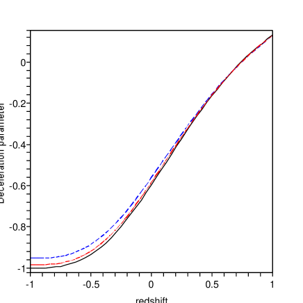
This equation shows that $\dot{E}<0$ for all $z$, as in the LDGP case, and that $\dot{E}\to 0$ as $z\to-1$ (equivalently, as $a\to\infty$), for all $w_{\text{q}}\geq-1$. This behaviour is illustrated in Fig. 1. Thus there is no super-acceleration, and no big rip singularity in QDGP models. The purely gravitational phantom behaviour does not produce the pathologies associated with phantom matter in GR.

Since $\dot{E}$ is always negative, the deceleration parameter, $q=-(1+\dot{E}/H_{0}E^{2})$, can be never less than $-1$, as seen in Fig. 1. Note that the asymptotic future value of $q$ depends on $w_{\text{q}}$:

$$q\to 3(1+w_{\text{q}})-1~{}~{}\text{as}~{}~{}z\to-1\,.$$ (15)

The transition redshift $z_{\text{a}}$ at which decelerated expansion turns into accelerated expansion, is defined by $q=0$, i.e.,

$$\dot{E}(z_{\text{a}})=-H_{0}E(z_{\text{a}})^{2}\,.$$ (16)

For the parameter values in Fig. 1, $z_{\text{a}}\sim 0.7$.

The QDGP and LDGP models show an important difference in the asymptotic behaviour of the Hubble rate:

$$E\to\left\{\begin{array}[]{cll}0\,,&$~{}~{}$&w_{\text{q}}>-1\,,\\ \sqrt{\Omega_{r_{c}}+\Omega_{\Lambda}}-\sqrt{\Omega_{r_{c}}}>0\,,&&w_{\text{q}}=-1\,.\end{array}\right.$$ (17)

In LDGP models, the de Sitter solution is a stable attractor. This arises because the vacuum energy does not redshift. By contrast, in QDGP models we have $H\to 0$, since the quintessence is redshifting away.

Figure 2: The equivalent GR phantom potential $V_{\text{eff}}(z)$ for the parameter values in Fig. 1.

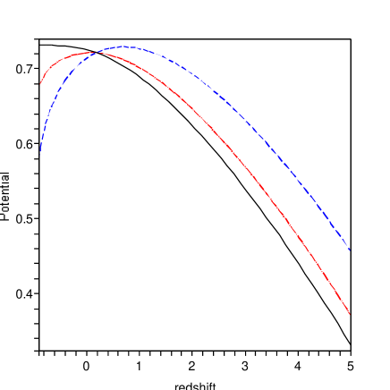
The quantities $\rho_{\text{eff}}$ and $w_{\text{eff}}$ describe a phantom scalar field $\phi_{\text{eff}}$ in GR which has the equivalent expansion history to the QDGP model. We can find the self-interaction potential $V_{\text{eff}}(\phi_{\text{eff}})$ of the equivalent GR phantom field by using the well-known result that a scalar field and its potential may be determined for any given expansion history as follows Ellis:1990ws :

$$\frac{V_{\text{eff}}(z)}{3H_{0}^{2}}=E^{2}-\Omega_{\text{m}}(1+z)^{3}-\frac{d[E^{2}-\Omega_{\text{m}}(1+z)^{3}]}{2\;\;d\ln(1+z)^{3}},$$ (18)

$${\phi_{\text{eff}}(z)\over\sqrt{3}}=-\int\frac{dz}{(1+z)E}\left[\frac{d[E^{2}-\Omega_{\text{m}}(1+z)^{3}]}{d\ln(1+z)^{3}}\right]^{1/2}.$$ (19)

In principle, these equations lead to $V_{\text{eff}}=V_{\text{eff}}(\phi_{\text{eff}})$, but in practice the inversion cannot be performed analytically because of the integral in Eq. (19). In Fig. 2 we show $V_{\text{eff}}(z)$. For the LDGP model, $V_{\text{eff}}$ approaches a constant nonzero value as $a\to\infty$. By contrast, in the QDGP model the potential vanishes asymptotically.

III Dynamical System Analysis

In order to write the cosmological equations in the form of an autonomous system, we define the following expansion normalized variables:

$$x=\frac{\sqrt{\Omega_{\text{m}}}}{a^{3/2}E}\,,~{}y={\frac{\sqrt{\Omega_{\text{q}}}}{a^{3(1+w_{\text{q}})/2}E}}\,,~{}v={\frac{\sqrt{\Omega}_{r_{c}}}{E}}\,,$$ (20)

so that Eq. (12) becomes

$$2v=x^{2}+y^{2}-1\,.$$ (21)

This constraint means that the phase space is defined by $x^{2}+y^{2}\geq 1$, since $v\geq 0$, and by $x\geq 1,y\geq 1$. Introducing the new time variable $\tau=\ln a$, and eliminating $v$ and $E$, we obtain the autonomous system

$$x^{\prime} = \frac{3x\left[x^{2}+(1+2w_{\text{q}})y^{2}-1\right]}{2(x^{2}+y^{2}+1)},$$ (22)

$$y^{\prime} = \frac{3y\left[2x^{2}+(1+w_{\text{q}})(y^{2}-x^{2}-1)\right]}{2(x^{2}+y^{2}+1)}.$$ (23)

The analysis depends on whether $w_{\text{q}}>-1$ or $w_{\text{q}}=-1$.

Table 1: Fixed points for $0>w_{\text{q}}>-1$.

Point	$(x,y)$	Eigenvalues	Character
$M$	$(1,0)$	$\left(-\displaystyle\frac{3w_{\text{q}}}{2},\displaystyle\frac{3}{2}\right)$	repellor
$Q$	$(0,1)$	$\left(\displaystyle\frac{3w_{\text{q}}}{2},\displaystyle\frac{3(1+w_{\text{q}})}{2}\right)$	saddle

Table 2: Fixed points for $w_{\text{q}}=-1$.

Point	$y$	Eigenvalues	Character
$M$	$0$	$\displaystyle\frac{3}{2}$	repellor
$dS$	$\sqrt{\Omega_{r_{c}}/\Omega_{\Lambda}}+\sqrt{1+\Omega_{r_{c}}/\Omega_{\Lambda}}$	$-3$	attractor

Figure 3: Phase plane trajectories for $w_{\text{q}}=-0.8$.

Figure 4: Phase line trajectories for $w_{\text{q}}=-1$, $\sqrt{\Omega_{r_{c}}/\Omega_{\Lambda}}=21$.

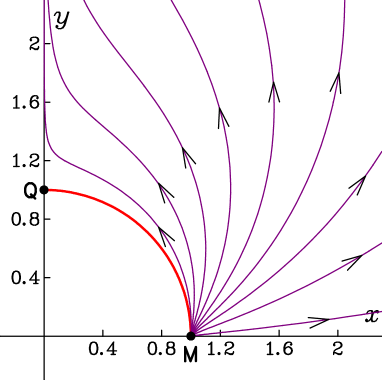
For $w_{\text{q}}>-1$, the phase space is 2D. The fixed points and their stability are summarized in Table 1. In this case there are two isolated fixed points located at finite values of $x$ and $y$. Combining this fact with a simple examination of the $y^{\prime}$ equation and the open topology of the phase space, we can draw fairly general conclusions about the properties of the fixed points of the system even before doing the linear analysis. Since $y>0$ and $w_{\text{q}}>-1$, we have $y^{\prime}>0$, so that the fixed points cannot be stable. In addition, the fixed points cannot be unstable spirals or centres, so they can only be unstable nodes (attractors) or saddle points. The linear analysis confirms these findings. The fixed points $M$ (early time) and $Q$ (late time) are matter- and quintessence-dominated solutions respectively. The phase plane trajectories are illustrated in Fig. 3.

For the LDGP limit, $w_{\text{q}}=-1$, we have $y\propto v$, leading to a 1D phase space, and the dynamical equations reduce to

$$y^{\prime}=\frac{3y\left(1-y^{2}+2\sqrt{\Omega_{r_{c}}/\Omega_{\Lambda}}\,y\right)}{2\left(1+\sqrt{\Omega_{r_{c}}/\Omega_{\Lambda}}\,y\right)}.$$ (24)

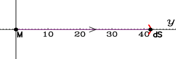
There are also two isolated fixed points at finite values of $y$ (see Table 2 and Fig. 4). It can be seen that $y^{\prime}>0$ as well, but since the phase space is only a line segment, and the fixed points are just its end points, it follows that one fixed point will necessarily be unstable (the matter-dominated point $M$), and the other will be forced to be stable (the de Sitter attractor $dS$).

IV Crossing the Phantom Divide

Perhaps the most distinctive feature of the QDGP model is the possibility of crossing the phantom divide $w=-1$. This occurs with non-phantom quintessence, via the infrared gravitational modifications to GR. In the standard GR model, this can be realized only by introducing additional complicated features like multiple dark energy fields or interactions between dark energy and CDM.

Figure 5: The effective dark energy equation of state $w_{\text{eff}}(z)$ for the same parameter values as in Fig. 1.

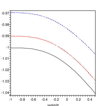
Equation (7) defines the effective equation of state, which leads to

$$\!\!\!\!\!\!\!1+w_{\text{eff}}(z)=$$

$$\!\!\!\!\!\!\!\frac{(1+w_{\text{q}})\Omega_{\text{q}}E(z)(1+z)^{3w_{\text{q}}+3}-\sqrt{\Omega_{r_{c}}}\Omega_{\text{m}}(1+z)^{3}}{\left[E(z)+\sqrt{\Omega_{r_{c}}}\,\right]\left[\Omega_{\text{q}}(1+z)^{3w_{\text{q}}+3}-2\sqrt{\Omega_{r_{c}}}E(z)\right]}\!.$$ (25)

For the LDGP model, i.e., the $w_{\text{q}}=-1$ limit of QDGP, $w_{\text{eff}}$ is always more negative than $-1$, provided that $\rho_{\text{eff}}>0$. When $\rho_{\text{eff}}=0$, at some redshift $z_{*}$, we have $w_{\text{eff}}=-\infty$. For $z>z_{*}$, we have $w_{\text{eff}}>-1$, with $w_{\text{eff}}\to+\infty$ as $z\to z_{*}$. Thus $w_{\text{eff}}$ never passes through $-1$.

For $w_{\text{q}}>-1$, the nonzero term $(1+w_{\text{q}})\Omega_{\text{q}}E(z)(1+z)^{3w_{\text{q}}+3}$ in Eq. (25) allows for $w_{\text{eff}}$ to pass through $-1$. This is illustrated in Fig. 5. For $w_{\text{q}}>-1$, smooth crossing of the phantom divide occurs at a redshift $z_{\text{c}}$ that depends on the values of the free parameters $\Omega_{\text{m}}$, $\Omega_{\text{q}}$ and $w_{\text{q}}$. By Eq. (25), $z_{\text{c}}$ is given by

$$(1+z_{\text{c}})^{3w_{\text{q}}}E(z_{\text{c}})=\frac{\Omega_{\text{m}}\sqrt{\Omega_{r_{c}}}}{(1+w_{\text{q}})\Omega_{\text{q}}}\,.$$ (26)

Note that for LDGP ($w_{\text{q}}=-1$), the solution is $z_{\text{c}}=-1$, i.e., crossing occurs at $a=\infty$.

At a redshift $z_{*}>z_{\text{c}}$, we have $\rho_{\text{eff}}(z_{*})=0$, so that the effective phantom GR picture of QDGP breaks down:

$$z_{*}=\left(\frac{4\Omega_{r_{c}}\Omega_{\text{m}}}{\Omega_{\text{q}}^{2}}\right)^{1/3(21+w_{\text{q}})}-1\,.$$ (27)

As in the LDGP case, we have $w_{\text{eff}}\to\mp\infty$ as $z\to z_{*}^{\mp}$.

V Conclusions

The DGP$(-)$ class of braneworld models can lead to phantom-like behaviour of the effective dark energy, but without the need for any phantom matter, as pointed out by Sahni and Shtanov Sahni:2002dx . In the simplest LDGP model, the universe contains only cold dark matter and a cosmological constant. We generalized this by introducing a quintessence field, to define the QDGP model. QDGP has the same effective phantom behaviour as LDGP. The Hubble parameter is always decreasing, and there is no big rip singularity in the future. The key new feature of QDGP is crossing of the phantom divide, $w=-1$, which is not possible in the LDGP case.

The avoidance of any big rip is due to $H,\dot{H}\to 0$ as $a\to\infty$. This asymptotic behaviour reflects the fact that the phantom effects never dominate – unlike the case of a phantom scalar field in GR. The total equation of state parameter, defined by $w_{\text{tot}}=p_{\text{tot}}/\rho_{\text{tot}}=w_{\text{eff}}\rho_{\text{eff}}/(\rho+\rho_{\text{eff}})$, follows from Eqs. (12) and (25),

$$1+w_{\text{tot}}(z)=$$

$$~{}{\Omega_{\text{m}}(1+z)^{3}+(1+w_{\text{q}})\Omega_{\text{q}}(1+z)^{3(1+w_{\text{q}})}\over E(z)\left[\sqrt{\Omega_{r_{c}}}+E(z)\right]}\,.$$ (28)

This shows that $w_{\text{eff}}(z)\geq-1$.

Acknowledgements
We thank Mariam Bouhmadi-Lopez for useful discussions. LC, RL and IQ thank the ICG, Portsmouth for hospitality while this work was initiated. The visit of IQ was supported by the Royal Society. This work has been carried out with the partial support of the Spanish Ministry of Science and Education through research grants FIS2004-0374-E. RL is supported by the Spanish Ministry of Science and Education through the RyC program, and research grants FIS2004-01626 and FIS2005-01181.