WIDE-FIELD CORRECTOR FOR A GREGORY TELESCOPE

Abstract — A form of prime focus corrector for the Gregory system is proposed that provides the sub-arcsecond field of view up to $3^{\circ}$ in diameter for the spectral range $0.35-0.90$ microns. The corrector includes five lenses made of same glass (fused silica is preferable). The distinctive feature of the corrector consists in dissimilar use of the central and edge zones of a front lens disposed in the exit pupil of a two-mirror system.

As an example, the f/1.9 telescope is considered with the 6.5-m aperture and the total length 8.8 m. Its primary and secondary mirrors are pure ellipsoids close to concave paraboloid and concave sphere, respectively. In the basic configuration, all surfaces of the corrector are spherical. The diameter of a star image $D_{80}$ varies from $0^{\prime\prime}.25$ on the optical axis up to $0^{\prime\prime}.50$ at the edge of the $2^{\circ}.3$ field. Only slightly worse images shows spherical corrector for the $2^{\circ}.4$ field of view. The fraction of vignetted rays grows on 1.7% from the center of field to its edges. Aspherization of some lens surfaces allows to reach sub-arcsecond images in the field of $3^{\circ}.0$ in diameter.
©  2006 MAIK “Nauka/Interperiodica”.

Key words: telescopes, astronomical observing techniques, devices and instruments

Introduction

Recent designs of lens correctors for the large telescopes provide the field of view of sub-arcsecond image quality up to $3^{\circ}$ in a Cassegrain system (Hodapp et al., 2003), in a three-mirror Mersenn–Schmidt system (Paul, 1935; Willstrop, 1984; Angel et al., 2000; Seppala, 2002), and in a prime focus of hyperbolic mirror (Terebizh, 2004). In the two former cases, a telescope is quite compact, while the surfaces of mirrors and lenses are complicated. In the latter case, it is possible to achieve the above field even at all spherical lenses, but the telescope length is about focal length of its primary mirror.

The Gregory system (both classic, with a paraboloidal primary, and aplanatic, with ellipsoidal surfaces of the mirrors) has an attractive feature: its exit pupil is not imaginary, as it takes place for the Cassegrain system, but real. Usually, the Gregorian exit pupil is situated not far from the primary focus. Such a position allows us to place a correcting optical element directly in the exit pupil, providing efficient correction of aberrations of a two-mirror system without auxiliary optics.

At first glance, the superposition of wide light beams near the primary focus prevents to imposing a lens corrector in the Gregory system (see Fig. 1). However, as shown below, it is possible to avoid additional obscuration, if we make a hole at the center of the front lens of the corrector and shift the rear its part to the primary mirror. As a result, we obtain a wide-field catadioptric system that combines compactness with simple shape of the optical surfaces. The system provides the sub-arcsecond field of view ${\sim 2^{\circ}.5}$ in diameter even at all-spherical corrector. It is worth noting that the spherical corrector for the Gregory system repeats the lens corrector that was proposed earlier for a single hyperbolic mirror (Terebizh, 2004). Subsequent aspherization of some lens surfaces allows to achieve the field about $3^{\circ}$ in diameter.

In present paper, we discuss the Gregorian corrector with an example of a 6.5-m telescope with the focal ratio $\phi\equiv F/D\simeq 1.9$. The effective focal length of the telescope, $F\simeq 12.4$ m, allows to fit resolutions of the optics and actual light detectors. The corrector consists of five lenses made of the same, virtually any material. At use fused silica and simple coating as a $MgF_{2}$ single layer, the telescope light transmission reaches 70%. The detector window has some optical power, the field is slightly curved, that is quite allowable, taking into account its linear size: approximately 0.5 m.

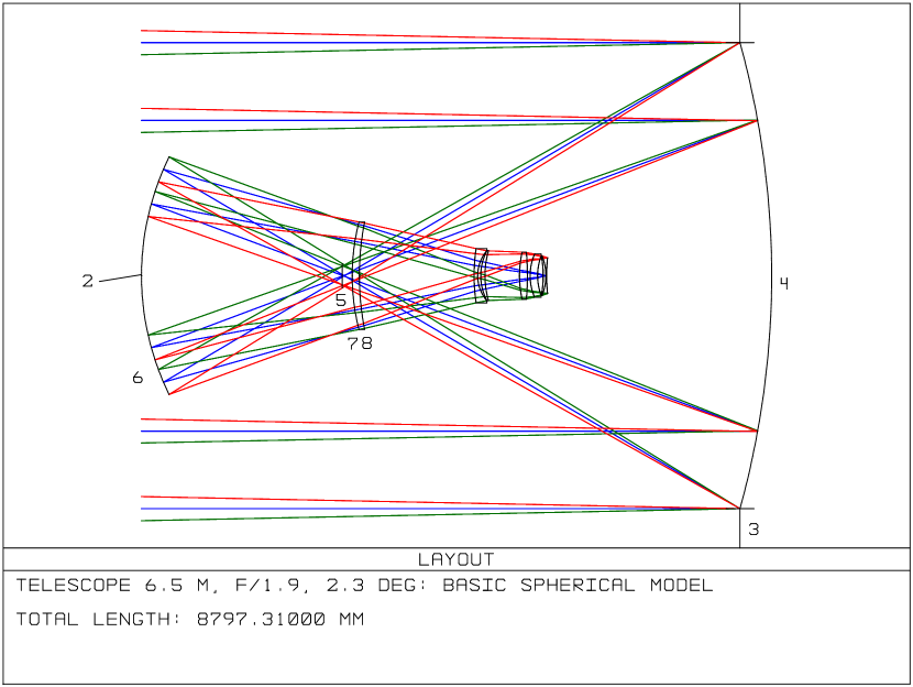
Figure 1: *

Optical layout of the 6.5-m telescope with the spherical basic corrector. Ordering of the surfaces corresponds to the Table 2.

Basic system of the 6.5-m telescope

In a basic configuration of the telescope (Figs. 1, 2), the primary and secondary mirrors are pure ellipsoids, while the lens surfaces are spherical. General performance of the telescope for a case, when the field of view is $2^{\circ}.3$ in diameter, is given in the Table 1; the parameters of its optical layout are specified in the Table 2. At the description of the optical layout we have introduced, for convenience, a fictitious surface No. 5, located close to the paraxial primary focus.

Figures 3 and 4 show image quality provided by the basic system, optimized for the field of view $2^{\circ}.3$. The circle diameter that contains 80% of a stellar image energy (designed, as usually, by $D_{80}$), varies within the waveband $0.35-0.90\,\mu$m from $\sim 0^{\prime\prime}.25$ at the center of the field up to $\sim 0^{\prime\prime}.50$ at its edge. The linear coefficient of central obscuration $\eta=0.51$, so the effective aperture diameter of the system is 5.6 m. The fraction of vignetted rays enlarges from the center of field to its edge less than on 2%.

Table 1. Basic system of the 6.5-m telescope
	Waveband, $\mu$m
Parameter
	0.35 – 0.45	0.54 – 0.66	0.70 – 0.90
Field of view
Angular	$2^{\circ}.3$
Linear	498 mm
Effective focal length, mm	12370.7	12368.9	12367.8
Relative focal length	1.903
Length of the system	8797.3 mm
Scale, $\mu$m/arcsec	59.97	59.97	59.96
Relative vignetting
at the edge of field	1.7 %
Variation of the RMS	$5.9-14.7\,\mu$m	$5.0-8.0\,\mu$m	$5.4-11.0\,\mu$m
image radius over field	$0^{\prime\prime}.10-0^{\prime\prime}.25$	$0^{\prime\prime}.08-0^{\prime\prime}.13$	$0^{\prime\prime}.09-0^{\prime\prime}.18$
Variation of $D_{80}$ from the	$15.8-31.6\,\mu$m	$14.4-22.1\,\mu$m	$16.8-29.7\,\mu$m
center to the edge of field	$0^{\prime\prime}.26-0^{\prime\prime}.52$	$0^{\prime\prime}.24-0^{\prime\prime}.37$	$0^{\prime\prime}.28-0^{\prime\prime}.50$
Transmission with the
single layer of $MgF_{2}$	$0.70$	$0.71$	$0.70$
Maximum distortion	0.27 %	0.28 %	0.29 %
The lens surfaces	All spheres

The relative focal length of the primary mirror, $\phi_{1}\equiv F_{1}/D_{1}$, is about 0.92, for the secondary mirror we have $\phi_{2}=0.56$. Let us remind, for comparison, relative focal lengths of three mirrors of the Large Synoptic Survey Telescope (LSST) according to Seppala (2002): $1.057$, $0.914$ and $0.774$; the light diameters are $8.40$ m, $3.37$ m and $5.44$ m, respectively. These mirrors are aspherics of the 6th–10th orders, the secondary mirror is convex. The primary mirrors of the Large Binocular Telescope (LBT) of diameter 8.4 m have $\phi_{1}=1.14$ (Hill, 1996; Salinari, 1996).

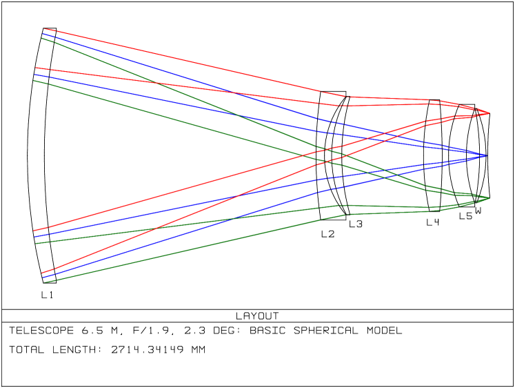
Figure 2: *

Optical layout of the basic corrector. Numbers of lenses
correspond to the Table 2, the detector window is marked by ‘W’.

According to the above data, we expect no specific problems at manufacturing of monolithic primary for the proposed here system, but the secondary mirror seems to be dangerously fast. However, we have to take into account that both mirrors are the concave pure ellipsoids, which can be controlled during manufacturing with the aid of the well-known and reliable methods. The other aspect of the problem under discussion concerns the customary nowadays practice of including the secondary mirrors to the active optics systems (e.g., on the LBT). These mirrors properly change their shape under action of actuators, and have very complicated form at each moment of time. For this reason, the initial form of a secondary mirror in active system is not obliged to follow the exact design. Further, it is known that making of fast mirrors becomes strongly simpler at use of the mosaic technology (see, e.g., Mountain and Gillett, 1998; Wilson, 1999). Let us notice, at last, that the f/number of a secondary depends upon a set of general characteristics of a telescope, and, in case of need, one can initially choose the characteristics in such a way that $\phi_{2}$ gets the desirable range. All said above allows to hope, that manufacturing of a secondary mirror for the proposed system is within modern technological abilities.

Table 2. Parameters of the basic 6.5-m telescope, optimized for the field $2^{\circ}.3$
Number		Curvature	Thickness		Light	Conic
of the	Comments	radius	(mm)	Glass	diameter	constant
surface		(mm)			(mm)
1	Screen	$\infty$	0	—	3315.00	0
2	Vertex of
	secondary	$\infty$	8355.89	—	0	0
3	Aperture
	diaphragm	$\infty$	441.42	—	6500.00	0
4	Primary	$-11993.55$	$-5995.78$	Mirror	6500.00	$-0.866870$
5	Primary focus	$\infty$	$-2801.53$	—	338.43	0
6	Secondary	$3728.74$	$2941.53$	Mirror	3314.54	$-0.194002$
71)	L1	$3034.14$	$100.00$	FS3)	1500.00	0
82)		$3835.23$	$1601.82$	—	1466.74	0
9	L2	$2587.74$	$50.00$	FS	758.08	0
10		$541.32$	$42.41$	—	697.64	0
11	L3	$736.49$	$59.65$	FS	698.08	0
12		$1268.16$	$481.986^{4)}$	—	693.44	0
13	L4	$1532.40$	$110.00$	FS	655.58	0
14		$-3638.17$	$37.74$	—	644.04	0
15	L5	$747.81$	$105.00$	FS	601.65	0
16		$800.48$	$78.00$	—	553.91	0
17	Window	$-1452.45$	$37.71$	FS	553.05	0
18		$-727.49$	$10.00$	—	551.45	0
19	Detector	$2322.90$			498.01	0

¹⁾ The hole of 427.7 mm in diameter.
²⁾ The hole of 542.3 mm in diameter.
³⁾ $FS$ – fused silica.
⁴⁾ The visual waveband is meant. The distances for the blue and red wavebands are 482.011 mm and 481.936 mm, respectively.

Figure 3: *

Spot diagrams of the 6.5-m telescope with spherical basic corrector
for the field angles $0;\,0^{\circ}.3;\,0^{\circ}.6;\,0^{\circ}.9$ and $1^{\circ}.15$ (the rows). The columns correspond to the wavebands $0.35-0.45\,\mu$m, $0.54-0.66\,\mu$m and $0.70-0.90\,\mu$m, respectively. The box width is $1^{\prime\prime}$ ($60\,\mu$m).

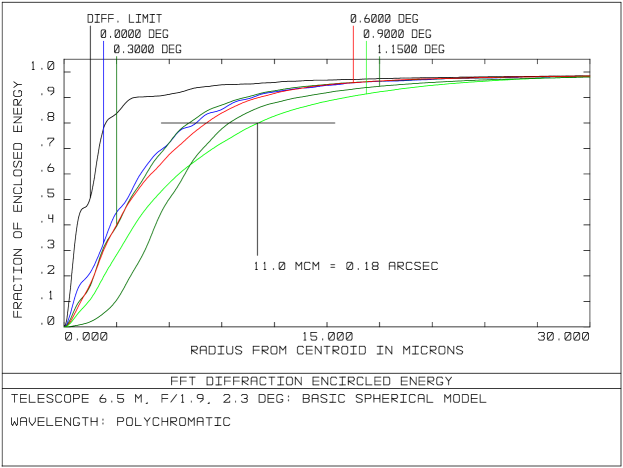
Figure 4: *

Basic telescope: Integral energy distribution along radius in a star image for the waveband $0.54-0.66\,\mu$m and the field angles $0;\,0^{\circ}.3;\,0^{\circ}.6;\,0^{\circ}.9$ and $1^{\circ}.15$. The similar distribution in the diffraction-limited image and the $80\%$-level are also shown.

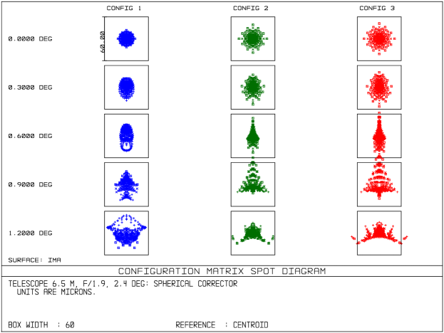
Figure 5: *

Spot diagrams of the 6.5-m telescope with spherical corrector for the
field angles $0;\,0^{\circ}.3;\,0^{\circ}.6;\,0^{\circ}.9$ and $1^{\circ}.2$ (the rows). The columns correspond to the wavebands $0.35-0.45\,\mu$m, $0.54-0.66\,\mu$m and $0.70-0.90\,\mu$m, respectively. The box width is $1^{\prime\prime}$ ($60\,\mu$m).

Figure 6: *

Spot diagrams of the 6.5-m telescope with aspheric corrector for the
field angles $0;\,0^{\circ}.5;\,0^{\circ}.75;\,1^{\circ}.0$, $1^{\circ}.25$ and $1^{\circ}.50$. The columns correspond to the wavebands $0.35-0.45\,\mu$m, $0.54-0.66\,\mu$m and $0.70-0.90\,\mu$m, respectively. The box width is $1^{\prime\prime}$ ($60\,\mu$m).

The aperture diameter and general characteristics of the telescope were mainly determined by condition, that the diameter of the front corrector lens L1 (see Fig. 2) is no more than 1.5 m (the front lens of the LSST corrector is 1.34 m). A central cone-shaped hole should be made in L1 for passage of light beam reflected by the primary mirror. It is possible to manage without the hole, supposing double passage of light through the lens L1, but the image quality in a correspondingly optimized system is not so high.

Note that lens sizes are close to those in the prime focus corrector to a single hyperbolic mirror of 4 m in diameter (Terebizh, 2004). Thus, application of a Gregory corrector allows to essentially increase the telescope aperture – in this case from 4.0 m up to 6.5 m, – while the system length has decreased from 10.8 m down to 8.8 m.

The focal surface of about 0.5 m in diameter is a convex sphere of curvature radius about 2.3 m. The corresponding sag at the field edge is 13.4 mm. Relatively small field curvature does not prevent to placing a set of matrix detectors, which own sizes are less than $\sim 25$ mm.

There are a few ways to control focusing at change of the spectral range; we choose, as an illustration, variation of the distance between the third and forth lenses. Namely, according to the Table 2, one should shift the rear part of the corrector only by $+25\,\mu$m and $-50\,\mu$m to turn from the visible range to the blue and red wavebands, respectively.

Under the pixels size ${\sim 15\,\mu}$m, which is typical for the modern CCD’s, one pixel corresponds to $0^{\prime\prime}.25$. Thus, about $1-2$ pixels cover a star image of $D_{80}$ in diameter, and we may consider as feasible the matching of resolution of the optical system with that of the detector and the atmosphere image quality.

The telescope light transmission has been estimated, assuming the simple coatings – the single $\lambda/4$ layer of $MgF_{2}$. Of course, the modern multi-layer coatings will ensure best transmission of light.

It is important to note, that the corrector is close to an afocal system, so the optical power of the telescope is determined mainly by its mirrors. Evidently, just that feature allows to avoid chromatism and, as a consequence, to attain the large field of view. This general principle is true also for other catadioptric systems.

Extending the field of view

The all-spherical corrector provides the field up to about $2^{\circ}.5$. Fig. 5 depicts, as an example, the spot diagrams for the field $2^{\circ}.4$ in diameter. Comparison with the Fig. 3 shows that the image quality has worsened only a little. Further extension of the field meets difficulties caused, first of all, by accepted here restriction of the sizes of the corrector front lens.

As is well known, there is a quite simple, from a designer’s point of view, way to attain the more wide field of an optical system: the aspherization of the all or some surfaces. Certainly, this way complicates technical realization of the system. In particular, the tolerances becomes much more hard, so both the fabrication and use of the telescope is laborious. Ultimately, these factors have an essential effect on the cost of the telescope. Nevertheless, many large telescopes that are now in progress include polynomial aspherics up to 10th order. In our case, aspherization of some surfaces of the lens corrector, namely, adding the terms of 4th, 6th and 8th orders, provides the sub-arcsecond field of view about $3^{\circ}$ in diameter (Fig. 6).

Even the wider field of view is attainable by applying the polynomial aspherics not only on the lenses, but also onto the (concave) mirrors of the system. We shall not consider here this opportunity, as now the main task is to give the general description of the lens corrector for a quasi-Gregory telescope.

Concluding remarks

Let us estimate the throughput $E$ of the proposed telescope and, for comparison, that of the LSST and a 4-m one-mirror telescope. The frequently used now parameter $E$ is defined as product of the telescope effective area by the solid angle, corresponding to its field of view. Table 3 gives approximate values of $E$ for the two field sizes. All systems under consideration include the lens field correctors. Obviously, to continue discussion it is necessary to take into account also a number of concomitant factors, as that: a reality of manufacturing of the optical surfaces of required form, the tolerances on temporal stability of the whole set of parameters, the operation cost of a telescope etc.

Table 3. Throughput of some telescopes $(m^{2}\,deg^{2})$
	Field of view
Telescope
	$2^{\circ}.3$	$3^{\circ}.0$
One-mirror 4.0-m telescope
with a prime-focus corrector	46	78
Two-mirror 6.5-m Gregory with
the corrector at the exit pupil	102	170
Three-mirror 8.4-m LSST with
the three-lens corrector	–	264

It is worth mentioning, that the two-mirror telescope alone, taken as a part of the considered here catadioptric system, provides the image of an axial point-like object of $0^{\prime\prime}.15$ in diameter, but a quarter of degree off-axis image is already $6^{\prime\prime}$ in diameter. Nearly the same characteristics has the aplanatic version of a Gregory telescope without lens corrector.

In the Introduction, we have touched on the attractive features of the Gregory telescope: reality of its exit pupil and concave form of the secondary mirror. Let us remind also, that it is much easier in the Gregory system to design an efficient baffles than in the Cassegrain system (Terebizh, 2001).

Naturally, the described above 6.5-m telescope is only one of examples; our main purpose was to attract attention to possibility of versatile use of the central and periphery zones of the front lens of the corrector placed in the exit pupil of a two-mirror Gregory telescope. Proceeding from the basic configuration, it is possible to design systems with account of the particular conditions and auxiliary optics (e.g., filters and the atmospheric dispersion corrector). The scaling of the system to smaller diameters does not meet problems, but scaling to larger diameters causes increasing of the corrector front lens.

The author is grateful to V.V. Biryukov for useful discussions.

References

- [1] J.R.P. Angel, M. Lesser, R. Sarlot, T. Dunham, ASP Conf. Ser. 195, 81, 2000.
- [2] J.M. Hill, Proc. SPIE 2871, 57, 1996.
- [3] K.W. Hodapp, U. Laux, W. Siegmund, “Preliminary Design for the Pan-STARRS Telescope Optics”, Pan-STARRS Document Control PSDC-300-001-00, 2003.
- [4] M. Mountain, F. Gillett, Nature 395, Supp. A23, 1998.
- [5] M. Paul, Rev. Opt. Theor. Instrum. 14, 169, 1935.
- [6] P. Salinari, Proc. SPIE 2871, 564, 1996.
- [7] L.G. Seppala, Proc. SPIE 4836-19, 2002.
- [8] V.Yu. Terebizh, Experimental Astronomy 11, 171, 2001.
-
[9]
V.Yu. Terebizh, Astron. Letters 30, 231, 2004
(AURA-CTIO Report No. C10430A, 2003; arXiv: astro-ph/0402212). - [10] R.V. Willstrop, MNRAS 210, 597, 1984.
- [11] R.N. Wilson, Reflecting Telescope Optics, v. II. Springer, Berlin. 1999.