SPITZER Observations of z$\sim$3 Lyman Break Galaxies: stellar masses and mid-infrared properties

Abstract

We describe the spectral energy distributions (SEDs) of Lyman Break Galaxies (LBGs) at z$\sim$3 using deep mid-infrared and optical observations of the Extended Groth Strip, obtained with IRAC and MIPS on board Spitzer and from the ground, respectively. We focus on LBGs with detections at all four IRAC bands, in particular the 26 galaxies with IRAC 8 $\mu$m band (rest–frame K-band) detections. We use stellar population synthesis models and probe the stellar content of these galaxies. Based on best–fit continuous star-formation models we derive estimates of the stellar mass for these LBGs. As in previous studies, we find that a fraction of LBGs have very red colors and large estimated stellar masses (M${}_{*}>5\times$ 10¹⁰ M_⊙): the present Spitzer data allow us, for the first time, to study these massive LBGs in detail. We discuss the link between these LBGs and submm-luminous galaxies. We find that the number density of these massive LBGs at high redshift is higher than predicted by current semi-analytic models of galaxy evolution.

1 Introduction

In recent years, great advances in our understanding of the nature and evolution of high redshift galaxies have been made, thanks to the availability of large samples. The techniques that have been developed rely either on colour selection criteria (e.g. Steidel et al. 2003, 2004, Franx et al. 2003, Daddi et al. 2004) or detection in the submillimeter through blank field surveys using the Submillimeter Common User Bolometer Array (SCUBA) on the James Clerk Maxwell Telescope (JCMT, e.g., Hughes et al., 1998) or the Max-Planck Millimeter Bolometer array (MAMBO, e.g. Bertoldi et al 2000, Eales et al. 2000). All these surveys have unveiled large numbers of $z>2$ galaxies but the overlap between the various populations is by no means easy to investigate.

Among the various methods the Lyman break dropout technique (Steidel & Hamilton 1993), sensitive to the presence of the 912$\AA$ break, is designed to select $z\sim 3$ galaxies. The typical star formation rate (SFR) deduced from the UV continuum emission of Lyman break Galaxies (LBGs) is estimated to be moderate, around 20–50 M${}_{\odot}/$yr (assuming H₀=70 km s^-1Mpc^-1 and q₀=0.5). The SFR value quoted is the “mean” SFR which is derived from the entire LBG sample which ranges from 10 to 1000 M${}_{\odot}/$yr (for the most massive LBGs). There is clear evidence, however, for the presence of significant amounts of dust in LBGs (e.g. Sawicki & Yee 1998, Calzetti 2001, Takeuchi & Ishii 2004 ). When corrected for the presence of dust then this “mean” SFR values increase to $\sim$ 100 M${}_{\odot}/$yr. The high SFRs and co-moving density of LBGs, together with the results of the clustering analyses (e.g. Adelberger et al. 2004) makes them plausible candidates for the long-sought progenitors of present–day elliptical galaxies (e.g Pettini et al. 1998).

The nature of the relationship between LBGs and submm-luminous galaxies (hereafter SMGs) has, however, remained unclear. One possible scenario is the one where LBGs and SMGs form a continuum of objects with the submm galaxies representing the “reddest” dustier LBGs. Central to such a hypothesis is of course the issue of dust in LBGs. A number of techniques have been used to deduce the dust content of LBGs ranging from studies of the optical line ratios (Pettini et al. 2001) to formal fits of the overall SED of LBGs based on various star forming scenaria (e.g. Shapley et al. 2001, 2003). Both methods agree that the most intrinsically luminous LBGs, which have higher SFRs, contain more dust (e.g. Adelberger & Steidel 2000, Reddy et al. 2006). More recently, X-ray stacking studies have shown that intrinsically more luminous LBGs also contain more dust (e.g. Nandra 2002, Reddy & Steidel 2004). Another important issue in understanding LBG evolution and their connection to SMGs is the study of their stellar mass content. The co-moving stellar mass density at any given redshift is the integral of past star-forming activity. Thus, stellar mass is a robust tool to probe galaxy evolution and is subject to fewer uncertainties than the star formation rate (SFR).

Until recently, stellar mass estimates for z$\sim$3 LBGs have been based on ground–based photometry which only samples out to rest–frame optical band. The observed luminosity at these wavelengths is dominated by recent star-formation activity rather than the stellar population that has accumulated over the galaxy’s lifetime. With the advent of the Spitzer Space Telescope (hereafter Spitzer, Werner et al. 2004) we now have access to longer wavelengths. In particular the availability of the IRAC instrument (Fazio et al. 2004) with imaging capabilities out to 8 microns allow us to probe rest–frame K band (for z$\sim$3 galaxies) where the light is sensitive to the bulk of the stellar content. Preliminary results of adding IRAC photometry to stellar mass estimates have been presented in e.g. Barmby et al. (2004) for z$\sim$3 LBGs and Shapley et al. (2005) for BX$/$BM objects.

In this paper, we present sensitive mid–infrared photometry for a sample of spectroscopically confirmed z$\sim$3 LBGs detected as part of the IRAC Guaranteed Time Observations (GTO) program on the Extended Groth Strip (EGS). We focus on the broad band Spectral Energy Distributions (SEDs) of luminous LBGs detected with IRAC channel 4 (8 $\mu$m corresponding to rest–frame K–band). The sample benefits from deep ground based optical photometry and spectroscopy (Steidel et al. 2003). Our aim is to explore the range of stellar masses and assess the benefits of adding longer wavelength observations. We examine the correlation between mass and absolute luminosity (magnitude) from optical to the K–band. The paper is organised as follows: in Section 2 we present a brief account of the observations and data reduction while in Section 3 we review the sample properties followed by a discussion of the detailed SEDs (Section 4). We discuss the detailed models used to estimate stellar masses in Section 5 while in Section 6 we present the actual masses. We focus on the properties of massive LBGs in Section 7 and we discuss their possible evolution and connection to submm-luminous galaxies. We estimate the number density of these massive LBGs in Section 8 and summarize our conclusions in Section 9.

2 Spitzer Observations and Data Reduction

The IRAC (Fazio et al. 2004) data presented here were acquired as part of the IRAC GTO program. The Extended Groth Strip was observed by IRAC at 3.6, 4.5, 5.8 and 8.0 $\mu$m during January and July 2004. IRAC observations of the EGS cover an area of 2^∘$\times$10${}^{{}^{\prime}}$. IRAC on board Spitzer has the capability of observing simultaneously in the 4 bands, when scanning a region, with an effective F.O.V. of 5${}^{{}^{\prime}}\times 5^{{}^{\prime}}$. The IRAC exposures consisted of 52$\times$200 sec dithered exposures at each of the 3.8, 4.5, 5.8 $\mu$m wavelengths and 50$\times$208 sec exposures at 8$\mu$m, in the 2^∘$\times$10${}^{{}^{\prime}}$ map. Because the field was observed twice and at different position angles, removal of instrumental artifacts during mosaicing was significantly facilitated. The observations reach a (5$\sigma$) point-source sensitivity limit of 24.0, 24, 21.9, and 22.0 mag (AB) at 3.6, 4.5, 5.8 and 8.0 $\mu$m, respectively.

Observations with MIPS (Rieke et al. 2004) were carried out in June 2004 in scanning mode. The MIPS 24$\mu$m channel ($\lambda=23.7\mu$m; $\Delta\lambda=4.7\mu$m) uses a 128$\times$128 BIB Si:As array with a pixel scale of 2$\farcs$55 pixel^-1, providing a field of view of 5$\farcm$4$\times$5$\farcm$4. The scan map mode was used with the slow scan rate, which results in an integration time of 100 s pixel^-1 per scan pass (10 frames $\times$10 s) at 24 $\mu$m. Since the sky position angle of the scan direction is determined by the spacecraft roll angle, the observing dates were constrained such that the resulting scan map would extend along the position angle of the Groth Strip. The final scan maps cover a sky area of 2.4°$\times$10′ with integration times of $>700$ s at 24 $\mu$m. The 24$\mu$m point source sensitivity (5$\sigma$) is 70 $\mu$Jy.

The IRAC and MIPS Basic Calibrated Data (BCD) delivered by the Spitzer Science Center (SSC) include flat-field corrections, dark subtraction, linearity correction and flux calibration. The BCD data were further processed by each team’s own refinement routines. These additional reduction steps include distortion corrections, pointing refinement, mosaicing and cosmic ray removal by sigma-clipping. Source extraction was performed in the same way as described in Ashby et al. (2006). In brief, we used DAOPHOT to extract sources from both IRAC and MIPS images. With an FWHM of the Point Spread Function (PSF) of 1$\farcs 8$–2$\farcs 0$ for IRAC and 6$\arcsec$ for MIPS 24 $\mu$m, virtually all objects at high redshifts are unresolved. We performed aperture photometry using a 3$\arcsec$ diameter apertures for both IRAC and MIPS sources. The aperture fluxes in each band were subsequently corrected to total fluxes using known PSF growth curves from Fazio et al. 2004; Huang et al. 2004. The magnitudes presented in this work are all in the AB magnitude system.

3 The Spitzer LBG Sample

The EGS LBG sample was constructed from the LBG catalogue of Steidel et al. (2003). The catalogue was matched to the IRAC and MIPS source lists instead of doing direct photometry on the images. We searched for counterparts within a 2${}^{{}^{\prime\prime}}$ diameter separation centered on the LBG optical position. The typical size for an LBGs is about 1” and in most cases the LBG is clearly identified although in Section 6.1 we discuss those cases where multiple counterparts were present. Due to the resolution of 2” we do not anticipate finding many multiple component counterparts.

Steidel et al. (2003) have reported on the detection of 334 LBGs in the EGS area. The Spitzer EGS survey covers 244 LBGs. About 200 LBGs are detected with IRAC at 3.6$/$4.5 $\mu$m, 53 LBGs are detected with IRAC at 5.8 $\mu$m and 44 at 8.0 $\mu$m. Finally, 13 LBGs have counterparts in the MIPS 24 $\mu$m survey of the field. Of the initial sample of 244 LBGs observed by Spitzer in the EGS area 175 objects have confirmed spectroscopic redshifts and are identified as galaxies at z$\sim$3 (we stress that this number refers to objects classified as galaxies and that we exclude from our analysis those classified as AGN, QSO or stars). Among the 13 LBGs with MIPS detections, 6 objects are classified as galaxies at z$\sim$ 3 based on their optical spectra (of the remaining MIPS detections 3 are classified as QSO and 1 AGN).

In this paper we focus on the properties of 44 LBGs that have 8 µm detections (referred to hereafter as ”the 8 µm LBG sample”). Of these, 26 have spectroscopic redshifts. The 8 µm LBG sample includes seven of the nine galaxies detected by MIPS and in particular the Infrared Luminous LBGs (ILLBGs, Huang et al. 2005). The criterion for an LBG to be classified as ILLBG is detection at 24 µm, which for the sensitivity of the EGS survey ($\sim$70 $\mu$Jy (5$\sigma$) implies an infrared luminosity $L_{IR}>10^{11}$ L_⊙. The two LBGs with MIPS 24 $\mu$m detections but no 8 micron detection have not been added to the sample as their IRAC photometry is incomplete.

In Table 1 we list the ground based photometry for the 8 micron LBG sample. The UGRJK data and the spectroscopic redshifts come from the large compilation of Steidel et al (2003). In Table 2 we list the Spitzer photometry. The uncertainties in the IRAC $/$MIPS magnitudes were estimated from an analysis employing Monte-Carlo simulations. We added artificial sources to the images, extracted them in the same manner as real sources, and computed the dispersion between input and recovered magnitudes. The dispersion of the recovered magnitudes about the mean recovered magnitude, computed for each bin in input magnitude, were used as the uncertainty estimates. In Figure 1 we plot the rest–frame UV$/$optical$/$near-infrared SEDs of all LBGs in the EGS area. The SEDs are normalised in R magnitude (R=24 mag). The rest–frame UV (UGR) part of the spectrum shows relatively little variation. Although K-band magnitudes are available for $\sim$40% of the EGS LBG sample we note a range of R–K colors with a mean value of $<$R–K$>\sim$ 1.5.

Clearly, the addition of the Spitzer IRAC$/$MIPS bands improves dramatically our understanding of the nature of LBGs. The rest–frame near-infrared colors of LBGs are spread over 4 magnitudes. LBGs display a variety of colors ranging from those that are red with R-[3.6]$>$2 to blue with R-[3.6]$<$2. The SED of those LBGs with blue colors is rather flat from the far–UV to the optical with marginal (in 1 band) IRAC detections. On the other hand, the SEDs of the red LBGs are rising steeply towards longer wavelengths. It is worth noting, that a number of such red color LBGs display R-[3.6] values similar to the extremely red objects discussed by Wilson et. al. (2004). Most of the ILLBGs display such extreme colors (see discussion in Section 7.2 and Figure 1 of Huang et al. 2005). The Spitzer observations presented here show that a fraction of optically-selected LBGs ($\sim$30%) have red colors and have a higher dust extinction and higher masses in contrast to the majority of the LBG population which comprises mostly of objects with blue colors modest extinction and masses.

4 Population Synthesis Models

4.1 Model Parameters

The SEDs of the Spitzer detected z$\sim$3 LBGs cover a wide range in wavelength from $\sim$900$\AA$ to 2$\mu$m. In this Section we discuss the models used to fit their SEDs in order to investigate and constrain the star formation histories, extinction, and masses of the LBGs. We use the Bruzual & Charlot code (2003, hereafter BC03) to generate models in order to fit the LBG SEDs. The new BC03 models are based on a new library of stellar spectra with an updated prescription of AGB stars. As suggested by the authors we adopted the Padova 1994 stellar evolution tracks and constructed models with solar metallicity (see discussion in Shapley et al. 2004) and a Salpeter Intitial Mass Function (IMF) extending from 0.1 to 100 M_⊙. We use the Calzetti et al. (2000) starburst attenuation law to simulate the extinction.

A major uncertainty in this type of analysis is the parameterization of the star formation history (e.g. Papovich et al. 2001, Shapley et al. 2001, Bundy et al, 2005). For the present analysis we have considered mostly two simple single-component models: exponentially declining models of the form SFR(t) $\propto$ exp(-t$/\tau$) with e-folding times of $\tau$ = 0.05, 0.1, 0.5, 2.0, and 5.0 Gyr and, continuous star formation (CSF) models. Although complex models, such as combinations of various star forming histories or single bursts on top of a maximally old underlying bursts (as suggested by Papovich et al. 2001) are probably more realistic, we do not consider them in this work as we cannot constrain the model parameters easily.

Our main aim for each galaxy is to constrain the stellar population parameters. The fitted parameters are the following: dust extinction (parameterised by E(B–V)), age (t_sf defining the onset of star formation), stellar Mass (M_∗) and star formation history ($\tau$). Using BC03 we generate a grid of models with ages ranging between 1 Myr and the age of the Universe at the redshift of the galaxy in question and, varying extinction. For each set of E(B–V), star formation history, and age we derive a model with the full set of colors, UGRJK plus the IRAC 3.6, 4.5, 5.8 and 8 $\mu$m, placed at the redshift of the galaxy in question. The intrinsic model spectrum is then reddened by dust. The model SED is finally corrected for the intergalactic medium (IGM) opacity. The predicted colors are then compared with the observed ones using $\chi^{2}$ minimization technique. The best-fit E(B–V) and age combination was chosen to minimize $\chi^{2}$ and the intrinsic SFR and stellar mass were determined from the normalization of the best-fit model to the measured SED.

We estimated the confidence intervals for individual objects using Monte Carlo simulations. For each source we generated about 200 synthetic model SEDs of the data by varying the fluxes randomly (random values where chosen according the the Gaussian distribution of the measured uncertainties). We then repeated the fitting procedure for each new set and determined the 68% confidence intervals from the distributions of the best-fit values obtained with each set. The procedure used here is similar to the one used recently by Papovich et al. (2006) for DRGs, Shapley et al. (2001) and Papovich et al. (2001) for LBGs. We note a strong assymetry around best-fit values which we interpret as the presence of strong degeneracies especially between E(B–V) and t_sf (as we discuss in Section 5.2). We note however that, the inferred stellar mass is one of the best constrained quantities suffering much less from uncertainties involved with the specific star formation history used to describe a specific LBG. In what follows we discuss how varying properties of the model fits affect the best-fit SED parameters.

4.2 Extinction

The impact of different extinction laws has already been investigated by e.g. Papovich et al (2001), Dickinson et al. (2003) who found the effect to be overall small. For the present work we have adopted the Calzetti law since such a law reproduces the total SFR from the observed UV for the vast majority of LBGs (e.g. Reddy & Steidel 2004, Reddy et al., 2005, Nandra et al. 2003). The choice of the Calzetti law was also dictated by the desire to facilitate comparison with previous work in the field.

4.3 Initial Mass Function

As discussed in 4.1 we have chosen a Salpeter IMF for our stellar population models. In this Section we investigate the effect on the models when using different IMFs. A Scalo (Scalo 1986) or a Miller-Scalo (Miller & Scalo 1979) IMF are also consistent with the data, as long as we keep the model lower and upper mass cutoffs fixed at 0.1 and 100 M_⊙, respectively. Both the Scalo and the Miller-Scalo IMFs however, result in slightly younger ages than the ones obtained here using Salpeter IMF. A Chabrier IMF (Chabrier 2003), also behaves very similarly to the Salpeter IMF. Both of them have a very similar upper mass dependence. However, in the Chabrier IMF the low-mass end assumes a flatter behaviour, following a log-normal distribution. This IMF results in M$/$L ratios that are a factor of $\sim$1.5 smaller than those for a Salpeter IMF.

Overall the exact values of the upper$/$lower mass cutoffs have a more noticeable effect on the derived stellar masses. The major difference lies in the relative contribution of stars with M$<$M_⊙. A lower mass cutoff of 1M_⊙ would, for instance, result in stellar mass values that are lower by about 30–40% than those derived when the lower mass cutoff is set to 0.1M_⊙ (assuming a Salpeter IMF). The result would be more pronounced (i.e. the estimated stellar mass will be lower) if we use a Chabrier (2003) IMF instead. Bell et al. (2003) seem to favour a “diet” Salpeter IMF (a Salpeter IMF which is deficient in low mass stars) which in the local Universe provides a satisfactory explanation for the M$/$L ratios derived from colors. Since the stellar content of $z\sim 3$ galaxies and in particular the fraction of low-mass stars is presently unknown we do not investigate variations in the lower mass cutoff any further.

4.4 Metallicity

So far, information on element abundances in LBGs is rather limited. Pettini et al. (2002) determined element abundances in cB58, a typical L_∗ galaxy which benefits from a factor of 30 magnification, and found it to be $\sim$ 0.25 Z_⊙. Nagamine et al. (2001) suggested that near–solar metallicities are in fact common in z$\sim$3 galaxies with masses greater than 10¹⁰ M_⊙ which is broadly consistent with the results for cB58. Shapley et al. (2004) also argued for solar metallicities for z$\sim$3 LBGs. Because 8 µm-detected LBGs are likely to be more massive than the typical LBG at $z=3$, we used solar metallicity in the models. Reducing metallicity to half solar would decrease the derived masses by 10–20%.

4.5 Model Uncertainties

Besides photometric uncertainties the parameters derived from SED fitting suffer from systematics and are subject to degeneracies simply because the models cannot fully constrain the star formation history of a high redshift galaxy. The uncertainties are model-independent and plague even the simplest single-component models that we use in the present work. This is due to the fact that model parameters such as extinction and star formation are strongly dependent on the value of $\tau$ used to parameterise the star formation history.

The extinction E(B-V) is strongly dependent on $\tau$ and the exact prescription used to describe the star formation history. For example a decaying star formation model with a lower E(B-V) will produce the same G-R and R-K colors as a model with a larger $\tau$, smaller $\tau/$t_sf but a higher E(B-V). For constant star formation histories extinction is responsible for reddening the UV part of the spectrum which is made up of a mixture of stars of earlier types. Likewise, the inferred age, t_sf, for a given value of $\tau$ depends on the strength of the Balmer break. The latter is sensitive to the relative number of B, A and F stars with respect to late type stars and the CaII H and K absorption at  4000 $\AA$ (which is determined by the relative number of late type stars). A larger value of $\tau$ corresponds to older ages for the O and A stellar populations. Finally, the SFR also suffers from uncertainties since it is primarily derived from the UV slope which will correspond to different E(B-V) and dust attenuation factor depending on the assumed stellar population and extinction law.

The uncertainties we just discussed are of course likely to affect the inferred stellar masses but in a less dramatic way. Even in the case of single star formation histories (CSF or EXP) the derived stellar masses vary by a factor of $\sim$10% for different values of $\tau$. Uncertainties in extinction and age also influence the derived masses but, it is quite difficult to disentangle the effect each of these have on the masses. A highly extincted underlying stellar population will have a similar effect on the stellar mass as an older population. As we show in Section 5, the addition of rest-frame near-infrared photometry from Spitzer has helped to constrain the dust properties of 8 micron selected LBGs.

Uncertainties in the mass estimates become more serious when one assumes more complex star formation histories. Papovich et al. (2001), for instance, introduced underlying maximally old bursts with t${}_{sf}>>$$\tau$ and found an increase in the M$/$L by a factor of several without a noticeable effect on the UV colors. Glazebrook et al. (2004) introduced random bursts in the range of star formation histories used to fit their multiband photometry and found that the mass increased by about a factor of 2 although the amount by which the stellar mass is underestimated depends on the specific galaxy SED. We conclude that use of the simple star formation histories (CSF or EXP) is likely to provide a lower limit on the stellar mass estimate.

Finally, it is worth noting that stellar population models including the Thermally-Pulsating Asymptotic Giant Branch (TP-AGB) phase (Maraston 2005) can also be used to fit the SEDs of z$\sim$3 galaxies. The signature of the TP-AGB phase is quite prominent for ages 0.2–2 Gyrs and as van der Wel et al. (2005) points out they provide a better fit for the SEDs of their z$\sim$1 galaxies. We defer modelling of our z$\sim$3 LBGs with models including the TP-AGB phase for future work.

5 Stellar Masses

Using the stellar population synthesis models described in Section 5.1 we have estimated the stellar masses for the entire sample of 181 LBGs with confirmed spectroscopic redshifts. Figure 2 shows a histogram of the inferred stellar masses for the whole Spitzer LBG sample. From this sample we selected LBGs with 8 micron detections and carried out a detailed study of their properties. In Figure 3 we show the rest–frame UV–optical–near-IR SEDs together with best-fit models for the 8 micron LBG sample (26 objects with confirmed spectroscopic redshifts). In Table 3 we report the results from the best-fit stellar population models for each galaxy for the entire optical–IRAC SED. Parameters are listed for the best-fit model either CSF or exponentially decaying models, whichever gives the lowest value of $\chi^{2}$ with $\tau$ as a varying parameter. The stellar mass inferred from the best fit model along with the fit parameters for each object are reported in Table 3. The median age for our sample is t_sf = 700 Myr. More than 50% of our galaxies have t${}_{sf}>$ 500 Myr while only 15% have t${}_{sf}<$ 100 Myr.

As we discussed already in Section 3, the 8 micron LBG sample contains most (all but two) of the ILLBGs (Huang et al. 2005). ILLBGs appear to have red colors (R-[3.6]$>$3) and best-fit ages t${}_{sf}>$1000Myr. Using best-fit CSF models we compute the stellar masses of the ILLBGs and find them to be of the order of (M$>$10¹¹M_⊙). Extinction for these massive LBGs (parameterised by E(B–V)) is around 0.3. The fits of the ILLBGs are discussed in detail in Section 7.1. The inferred stellar masses quoted in Table 2 do of course suffer from the uncertainties discussed in Section 4.6 and are quantified with the error bars reported in the same Table. The median stellar mass for the 8 micron LBG sample is (8.16$\pm$1.04)$\times$10¹⁰ M_⊙ compared to (2.95$\pm$1.51)$\times$10¹⁰ M_⊙ estimated for the entire EGS-LBG sample (and excluding the 8 micron selected LBGs). The fraction of LBGs with M$>$5$\times$10¹⁰M_⊙ among the 8 micron LBGs is 40% compared to 25% for the entire EGS-LBG sample.

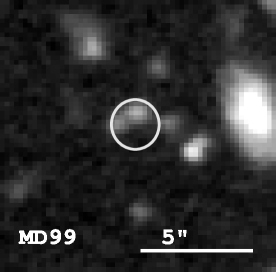
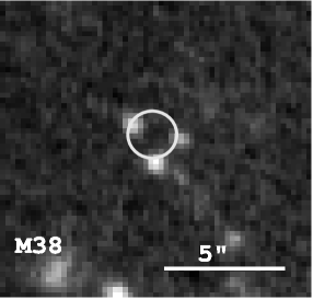
Figure 4: Subaru-R band postage stamps for two LBGs, Westphal-MD99 and Westphal-M38 where the 8 micron Spitzer flux might be contaminated due to the complex morphology of the sources. The images are 11$\arcsec\arcsec$ on a side and the circle indicates a 2 $\arcsec$ aperture.

Finally, it is also worth investigating the morphology of the 8 micron LBG sample. This investigation was carried out to assess at what level the IRAC fluxes might suffer from contamination from neighbouring sources. This is important as the resulting fluxes affect the modelling and the computation of stellar masses. For this reason we have compared the 8 micron IRAC images with deep R–band SUBARU images (Miyazaki, priv. comm). As we discussed in Section 2 the IRAC PSF is $\sim$2${}^{{}^{\prime\prime}}$ so we are looking for multiple sources within a 2${}^{{}^{\prime\prime}}$ area. Out of the 26 sources in the 8 micron LBG sample we have identified two cases where a possible contamination of the IRAC 8 micron flux by a neighbouring source is possible. In Figure 4 we show cutouts of the optical R-band images for Westphal-M38 and Westphal-MD99. While we include these sources in the discussion we caution that the reported fluxes might be contaminated.

5.1 Dust extinction: are 8 micron LBGs dustier?

In this Section we try to investigate the dust content of the 8 micron LBG sample based on the E(B–V) values derived from the best-fit models. In Figure 5 we plot the estimated stellar mass (based on best-fit CSF models) as a function of best-fit E(B–V) for the 8 micron LBG sample. We chose to plot E(B–V) against the stellar mass which, as we discussed extensively in Section 4, is relatively insensitive to the assumed star formation history. For comparison we also plot the same parameters for the LBG-EGS sample (i.e. all LBGs with detections in at least one IRAC band). The mean E(B–V) for the LBG-EGS, the 8 micron LBG and the ILLBG samples IS 0.156, 0.232 and 0.354, respectively. The more massive LBGs have, on average, higher E(B-V) though with a considerable scatter. We confirm that 8 micron LBGs suffer higher extinction (parameterised by the model value of E(B–V)) when compared to the Spitzer LBG sample (ie those without 8 micron detections). Moreover, extinction is higher for the ILLBGs although our sample is at present still small (6 objects) to draw statistically significant conclusions.

Another way to investigate the amount of obscuration in LBGs is to look at the 24 micron detections (ie the ILLBGs). Out of the 188 LBGs in the LBG-EGS sample only six of them are detected at 24 microns that is a fraction of $\sim$3%. However, the percentage of 24 micron detections among the 8 micron LBG sample is higher – 6 out of the 26 LBGs– which makes up for 23%. We thus conclude that Spitzer observations provide reliable means to probe the dust content of LBGs. In particular objects with Spitzer 24 micron detections must be in the high extinction end of the dust distribution.

6 Rest–frame NIR properties of LBGs

The addition of longer wavelength photometric points (ie the IRAC channels) has an effect on the accuracy of stellar mass estimates (e.g. Labbe et al. 2005, see also discussion in Section 7) but also on our understanding of the properties of the LBG population as a whole. Here, we investigate the distribution of stellar mass with rest–frame wavelength as we move from optical to the near-infrared bands. In Figure 6a we show the distribution of stellar masses as a function of absolute [3.6] $\mu$m magnitude which at the median redshift of 3 corresponds to rest–frame 0.9 $\mu$m (ie I–band). Although there is clearly a correlation between absolute I-band magnitude and stellar masses (correlation coefficient r=0.53) there is considerable scatter in the values especially at the fainter end. At the brighter end (which is where most of the massive galaxies are found) the correlation becomes tighter but this might also be due to the smaller number of sources at these magnitudes. We suggest that the spread in the correlation is due to the wide range of star–formation histories among LBGs. Moreover, it is apparent that it is quite difficult to project a single I-band rest–frame luminosity to a stellar mass.

In Figure 6b we show the distribution of stellar mass as a function of absolute [5.8] $\mu$m magnitude which at z=3 corresponds to rest–frame 1.4 $\mu$m (ie H–band). The correlation between stellar mass and absolute rest–frame H-magnitude improves significantly (r=0.61). The scatter in stellar mass decreases as one moves to longer wavelengths and probes the stellar luminosity due to recent$/$slightly older star formation activity. Likewise, in Figure 6c we plot the distribution of stellar masses as a function of absolute [8.0] $\mu$m magnitude which would correspond to rest–frame $\sim$2.0 $\mu$m (i.e. K–band). The correlation between stellar mass and magnitude becomes even tighter with r=0.77. The scatter in M$/$L values decreases and is now a factor of $\sim$12. The values of M$/$L for the most massive galaxies show a spread of about 10. From these simple comparisons, we conclude that the mid–infrared bands and especially the IRAC 8 $\mu$m channel (which samples the rest frame near–infrared wavelengths for z$\sim$3 LBGs) provides a more accurate estimate of the M$/$L ratio compared to that obtained when using optical bands. As we discussed already, IRAC 8 $\micron$ channel is sensitive to the light from the bulk of the stellar activity accumulated over the galaxy’s lifetime (see also Bell & de Jong 2001).

We finally examine the dependence of stellar mass on the R–[3.6] color index. As we discussed already in Section 5, the massive LBGs tend to have red colors with R–[3.6]$>$2. In Figure 6d we plot stellar masses as a function of the R–[3.6] color. The entire EGS–LBG sample (with confirmed spectroscopic redshifts) shows a wide range of R–[3.6] color with the 8 micron LBG members showing colors in the range 1 to 4. The most massive 8 micron LBGs (which are also ILLBGs) show the most extreme R–[3.6] colors $>$2.5. These values are close to the values of extremely red objects presented by Wilson et al. (2004). The correlation is tighter for the more massive$/$redder LBGs which have M$/$L close to that of present day galaxies.

All these results stress the importance of obtaining longer wavelength (rest–frame near-infrared) observations for the z=3 LBGs, as these allow us to probe the effect of recent star formation on the galaxy luminosities and masses. Although proper knowledge of the current stellar content is crucial, as we have discussed, it is the luminosity of older stars, that dominates the K–band light, that is found to correlate best with the derived stellar mass. In particular, this correlation becomes significant for the newly discovered ILLBGs and the massive 8 micron sample LBGs which have a significant dominant older stellar population. As we move to the other extreme of young and therefore less massive galaxies the current stellar content becomes perhaps more important as it dominates the luminosity and thus the stellar mass.

All the above correlations have been based on the stellar masses inferred from the models described in Section 3. To some extent the results are dependent on the particular details of the models assumed, in our case a single exponentially decaying or continuous episodes of star formation. Our models are, however, rather “conservative” in terms of the predicted stellar masses. If we use a two component model (an underlying old stellar episode and a very young continuous episode) this will result in a relative increase in the derived stellar masses which will be higher for the lower mass galaxies in comparison to the higher mass galaxies (Papovich et al. 2001, Shapley et al. 2005). This will likely make the trends seen in Figure 6 shallower but will not significantly affect our conclusions.

7 Comparison with K-selected LBGs

The original selection of LBGs was based purely on optical colors (Steidel & Hamilton 1992) thus only probing the rest–frame UV part of their spectrum. Shapley et al. (2001) and Papovich et al. (2001) obtained near-infrared photometry thus extending the available SEDs into the rest–frame optical. With the present data we have extended the SEDs of LBGs into the rest–frame near-infrared and have the opportunity to probe the bulk of the stellar emission. As we discussed already in Section 3 about 1$/$4 of the EGS-LBG sample has been detected with IRAC [8.0] (that probes the rest–frame K–band). In this Section, we want to compare the properties of the 8 micron LBG sample to those of optical$/$near infrared selected samples such as the NIRC sample (Shapley et al. 2001).

There are 16 LBGs in common between the NIRC (Shapley et al. 2001) and the entire LBG-EGS sample while five of these are part of the 8 micron LBG sample. Of these five targets we chose Westphal-D49 to carry out a detailed comparison. The best-fit CSF model for D49 (Table 3) has an age of t_sf=1350 Myr and an E(B–V) = 0.34. In the absence of the Spitzer photometry Shapley et al. fit D49 with a CSF model with 1139 Myrs and E(B–V)=0.17 In Figure 7 we want to compare the two models. It is obvious that in the absence of the Spitzer data both models would provide a good fit to the rest–frame UV–optical photometry. It is only with the addition of the rest–frame near infrared (Spitzer data) that a model with higher extinction becomes necessary. One could of course argue for a more “aged” and less extincted stellar model. Likewise, we have generated models where we varied the age of the stellar population (Figure 8). It is obvious that stellar ages larger than 1.3 Gyrs do not provide a satisfactory fit to the SED.

A similar exercise was performed for the remaining objects that are in common between the NIRC and our 8 micron LBG sample. For objects without 8 micron detections (11 LBGs) we find a very good agreement in the models (in particular age and extinction). The mean age of the NIRC sample is 355 Myrs compared to a mean age of 320 Myrs derived including the IRAC detections. Likewise the mean extinction derived for the NIRC sample is 0.218 whereas our mean extinction is 0.208. The differences are more pronounced however, for LBGs with 8 micron detections. Out of the small sample of 5 LBGs we derive mean age and extinction of 400 Myrs and E(B-V)=0.378, while the corresponding values for the NIRC fits are 293 Myrs and 0.238. For two of the five targets in common between NIRC and 8 micron samples (MD109 and MD115) Shapley et al. could not constrain the best-fit ages and thus fixed the age at 10 Myrs. Figure 9 summarizes our results.

The overlap between the NIRC sample and the 8 micron LBG sample is small so the differences might not be very significant. We suggest, however, that it is likely that LBGs with 8 micron detections have higher extinctions (see also discussion in 5.1) and slightly more aged population than LBGs undetected at 8 micron. The possibility for 8 micron contributions from a putative AGN cannot be constrained with the current data although optical spectroscopy (Steidel et al. 2003) or X-ray studies (e.g. Nandra et al. 2002) do not reveal any signs of such activity.

7.1 Massive LBGs and ILLBGs

A subset of the 8 micron LBG sample (12 objects out of 44) have masses M${}_{*}\geq$10 ¹¹ M_⊙. From this subset 1 object is a confirmed QSO and six objects do not have spectroscopic confirmation. In Section 5 we discussed in details the various models used and the accuracy in the derived stellar masses. In this Section we focus the discussion on these “massive” 8 micron LBG sample galaxies with confirmed spectroscopic redshifts. These massive 8 micron LBGs are also detected in the MIPS24 $\mu$m band. There are two additional galaxies that do not have 8 micron counterparts but are detected in the 24 MIPS band, we will consider those as part of the massive luminous LBG sample.

Because of their luminosity and rather unusual properties (compared to the rest of the LBGs) Huang et al. (2005) termed this subclass of objects as Infrared Luminous LBGs (ILLBGs). The masses of the ILLBGs have been estimated using BC03 models and are reported in Table 2. All ILLBGs are best fit by a CSF model with ages $>$ 1000 Myr with extinction that varies around A${}_{V}\sim$0.2. Although, as we discussed, the addition of the IRAC bands has significantly improved the accuracy of the derived stellar masses, the models do not constrain very well the star formation history of high-z and LBG objects (as has been discussed already by Papovich et al. 2001, Shapley et al. 2004, 2005). Despite the uncertainties in the detailed properties of the star formation history the derived stellar mass is a robust estimate depending mostly on the SED shape rather than the details of the particular model. However, we will show that in the case of these “massive” luminous LBGs we can, for the first time, discriminate between the two “simple” models (CSF vs EXP) used to fit the SEDs of the LBGs. We caution that although the star formation history of galaxies is a more complicated process than a constant star formation activity or a a smooth exponential function the details of more complicated models (short bursts of different strength superimposed on a constant star forming model) can not be well constrained so we do not consider them here.

As we have shown in Section 6 the correlation between estimated stellar mass and absolute magnitudes becomes tighter as one moves to longer wavelengths especially for the brighter more massive objects. An accurate estimate of the total stellar mass can be obtained when the star formation of the past several hundred Myrs is less than the integrated star formation over the lifetime of a galaxy. In a more realistic case, a good estimate of the stellar mass can be obtained when the light from the optical and more importantly near-infrared wavelengths far exceeds the UV light. The massive ILLBGs considered here represent exactly this phase in galaxy evolution: their light is dominated by the light of the older stars which output mainly in the near-infrared bands (observed frame around 8 $\mu$m covered by IRAC [8.0] channel) and exceed the light in the UV (due to the more recently formed stars). This is in line with the large M$/$L_2.2 found for the massive LBGs.

The last point to be addressed is the issue of the exact prescription of star formation history used to estimate masses for the ILLBGs. The discussion in Section 6 is of particular relevance. There, we discussed how the luminous (and massive) LBGs show the most extreme (very red) R-[3.6] and g-R colors. Through our detailed modelling we find that CSF models with an extinction E(B–V)$\sim$0.3, reproduce quite well the extreme colors of ILLBGs (see also Figure 2 in Huang et al. 2005). In models with declining star formation histories red G-R and R–[3.6] colous can be produced either with t${}_{sf}/\tau>$1 and little or no dust extinction or with smaller t${}_{sf}/\tau$ and more dust extinction. In such models the reddening of the UV slope is caused by a mixture of stars of later spectral types. In continuous star formation models reddening of the rest-frame UV is due solely to extinction. The fact that ILLBGs are detected at 24$\mu$m implies that they are quite dusty so that the constant star formation model provides a natural match to the extremely red colors observed. Since (observationally) we cannot constrain the spectral types of late type stars in LBGs we suggest that the CSF model is a better (simpler) explanation for the extremely red colors displayed by ILLBGs.

7.2 Old and Massive LBGs: a new class or the missing link?

We now want to investigate the connection between the massive luminous z$\sim$3 LBGs and the SMGs. Both LBGs and SMGs have sufficient SFRs to form present-day elliptical galaxies. Until recently, attempts to find a connection between the two populations had not been very successful (Webb et al. 2003, Chapman et al. 2000) although more recent studies (e.g. Chapman et al. 2005, Reddy et al 2005) have been exploring a possible link. Naturally, most of the submm searches targeted LBGs with high predicted SFRs. These SFRs, however, have been estimated based on the relationship between far-infrared$/$far-UV flux and UV continuum for local starbursts (Adelberger & Steidel 2000); this relationship however, does not apply to ultraluminous galaxies where a greater fraction of the total star formation is in optically-thick regions. Another issue is of course the detailed properties of the dust distribution in LBGs which may differ from that of present-day evolved galaxies (Takeuchi 2003). An obvious evolutionary scenario is one in which massive LBGs and SMGs form a continuum of objects with the bright submillimeter-selected sources representing the highest star-forming LBGs.

The current sample of massive LBGs has many properties in common with SMGs. For one, as we discussed in Section 6 their R–K colors are extreme ($>$3) similar to those of SMGs. Indeed the only LBG detected in the submm so far , Westphal -MMD11, by Chapman et al. (2000) shows such extremely red colors. The Spitzer colors of massive LBGs are also very similar to those of SMGs. Egami et al. (2004) reported on Spitzer detections of SMGs in the Lockman hole. Based on the observed SEDs of the SMGs and from comparisons with local templates they classified SMGs as warm (Mrk231-like SED) and cold (Arp220-like SED). They found that the majority of SMGs are cold. More recently, Ashby et al. (2006) presented a detailed study of the mid-colors of SMGs detected in the EGS area. Using these measurements as a reference point, we plot in Figure 10 (a and b) the R-[3.6] and [8.0]-[24.0] colors for SMGs and ILLBGs and find that they are indeed quite similar. For the SMGs we used the 17 candidates with secure 8 $\mu$ counterparts (see note in Table 1 of Ashby et al. 2006). Finally, it is worth looking at the inferred stellar masses of SMGs and LBGs: both populations appear to have large estimated stellar masses ranging from several $\times$10¹⁰ to 10¹¹ M_⊙ (e.g. Borys et al. 2005, Tecza et al. 2004). We caution that stellar mass estimates for SMGs are relatively uncertain due to the likely presence of an AGN component in some members. The values we quote are based on the estimates by Borys et al. (2005) for relatively young and gas-rich SMGs as well as the dynamical masses measured by Tecza et al. Based on the similarities of the colour indices, mid-infrared colors and inferred stellar masses we propose that a link must exist between ILLBGs and SMGs.

To further investigate the possible connection between the two populations let us also take a look at some sample statistics. Huang et al. (2005) found that ILLBGs represent about 15% of the total LBG population, excluding objects with possible contamination from AGN. This number most likely represents a lower limit to the true fraction of ILLBGs among the general LBG population for two reasons:(a) the MIPS depth is not uniform over all of the Steidel et al. (2003) fields and (b) we do not have spectroscopic confirmations for the whole ILLBG sample.

Recently, Chapman et al. (2005) presented spectroscopy of 73 SMGs with faint radio emission. The median redshift of the Chapman et al. sample is 2.2 with 19 objects with redshifts z${}_{spec}>$2.5. Although the redshift distribution of the SMGs does not match that of the z$\sim$3 LBGs we will use the Chapman sample as is the largest compilation of measured spectroscopic redshifts for SMGs (though we have to make some adjustments to allow for the slight difference in the mean redshifts) for our comparisons. Chapman et al. find that 30 of the 73 SMGs with confirmed spectroscopic redshifts have rest-frame UV-characteristics similar to those of star forming galaxies. Among the 19 z$>$2.5 SMGs, 6 of them have starburst-like UV colors (similar to those of LBGs). Thus, we estimate that $\sim$30% of SMGs are star-forming galaxies (with UV colors matching those of LBGs) with this number likely to be a lower limit (due to unidentified objects which are unlikely to show AGN signatures). Among the EGS-LBG sample, on the other hand, Huang et al. found that 15% of LBGs (the so-called ILLBGs) show evidence for increased dust extinction (via their 24 $\mu$m detections). Very recently we confirmed detection of ILLBGs at mm wavelengths with IRAM$/$MAMBO (Rigopoulou et al. 2006, in prep) at a flux level similar to that of faint SMGs.

Bringing these statistics together 30% of SMGs display LBG-like UV-colors while 15% of LBGs show evidence for higher extinction and submm emission. Thus, it is likely that ILLBGs (with red colors, higher A_V, submm emission) and a sub-fraction of SMGs (those with UV colors similar to starburst galaxies) appear to be identical in their UV and$/$or submm properties, this is likely to happen at the 2–3 mJy level. It is possible that SMGs fainter than the current survey limits (2-3 mJy) will have lower star formation rates and lower levels of dust obscuration, such that the overlap fraction between SMGs and LBGs would become increasingly larger as one goes to fainter flux levels. We suggest that an evolutionary or physical link between these two subsamples is likely to exist.

As a last point, we want to address the connection (if any) of ILLBGs with the DRGs (Franx et al. 2003). Foerster-Schreiber et al. (2004) and Labbe et al. (2005) compared the properties of DRGs and blue LBGs and found that the former are, not surprisingly, on average dustier and more massive. When examining the M$/$L_k mass-to-light ratio they find that DRGs display higher values (the mass-to-light ratios remains of course critically dependent on the assumed star formation history, metallicity and IMF values) than the LBGs. The mean age and extinction of DRGs is $<$t$>$=1.3 Gyr and $<$A${}_{V}>$1.5 mag. From the SED fits in Figure 2 of Labbe et al. (2005) we conclude that ILLBGs resemble more the “old and dusty” DRGs rather than the “dead” DRGs.

8 Massive LBGs: how many are there?

Recently, it has become apparent that the number densities of high-redshift galaxies with large stellar masses exceed the theoretical predictions of semi-analytical models of galaxy evolution (e.g. Saracco et al. 2004, Daddi et al. 2004, Tecza et al. 2004). In the widely accepted hierarchical merging scenario for galaxy formation, massive galaxies are the end points of mergers which increase with cosmic time. In the semi-analytical models of Kauffmann et al (1999), the predicted number density of $\mathcal{M}_{\rm star}\geq 10^{11}$ $M_{\odot}$ ellipticals at $z\simeq 2.5$ is about $5-6\times 10^{-5}$ Mpc^-3. A similar conclusion is reached by Moustakas & Somerville (2002). The semi-analytic models of galaxy formation in the hierarchical clustering scenario by Baugh et al. (1998, 2002) predict, in fact, no such massive galaxies at redshift z$>$2.

In Figure 11 we plot the evolution of the number density $\it{\Phi}(M>10^{11}M_{\odot})$ based on the massive LBGs (assuming an $\Omega_{m}=0.3$, $\Omega_{\Lambda}=0.7$ cosmology with H₀=70 km s^-1 Mpc^-1) as a function of redshift. If we assume an effective volume for the U-dropouts V = 450 h^-3 Mpc³ arcmin^-2 (taken from from Steidel et al. 1999) then, the effective co-moving volume becomes V = 1400 Mpc³ arcmin^-2 (the volumes have been weighted according to the number of objects per R-magnitude bin). For the 8 micron LBGs with M $>$10¹¹ M_⊙ in the 227 sq. arcmin Westphal field, we derive a co-moving density of $\Phi=(1.6\pm 0.5)\times 10^{-5}$ Mpc^-3 at the average redshift $\langle z\rangle\simeq 3$. The derived number density is an actual underestimate of the real number density of galaxies with $\mathcal{M}_{\rm star}\gtrsim 10^{11}$ $M_{\odot}$ at $z>3$ since our calculation refers only to the 8 micron selected massive LBGs. Although we are fairly confident that the 8 micron LBG sample contains all massive LBGs it does not, of course, account for the optically faint massive population at z$\sim$3. However, deriving $\Phi$ for other $z>3$ objects (e.g. the DRGs of Franx et al.) is a difficult task due to the very limited availability of measured spectroscopic redshifts for such targets. To date LBGs consitute by far the largest $z\sim 3$ sample with measured spectroscopic redshifts and thus we confined our calculations of the number density to this sample.

The current value of $\Phi$ is about a factor 3 higher than the predictions of hierarchical models by e.g. Kauffmann et al. (1999). In Figure 11 we also plot the co-moving densities of galaxies at z$\sim$0 (Cole et al. 2001), z$\sim$1 (Drory et al. 2004), z$\sim$2 (Fontana et al. 2004). In the same plot we show the theoretical predictions from semianalytical models of Kauffmann et al. (1999), and Baugh et al. (2003). It is evident from Figure 11 that the evolution of the number density of massive ( $\mathcal{M}_{\rm stars}\simeq 10^{11}$ $M_{\odot}$) galaxies with redshift is slower than the prediction of the current hierarchical models, at least in the redshift range 0$<$z$<$3. We note, however, that the number densities shown in Figure 11 are based on a variety of surveys with different selection techniques. This, undoubtedly, introduces selection biases. Although disentagling the various biases is beyond the scope of the present work, we stress that despite the selection effects the main conclusion regarding the number density $\Phi$ of z$\sim$3 galaxies remains unaffected.

The fact that these galaxies have already assembled this mass at z$\sim$3, places the possible merging event of their formation at z$\geq$3.5 assuming a dynamical time scale of 3$\times$10⁸ yr (e.g. Mihos & Hernquist 1996). The inferred mass weighted age of the stellar populations places the formation of their bulk at z${}_{f}\geq$ 3.5 implying substantial activity at such high redshifts. Ferguson et al. (2002) postulated that the assembly of massive systems at z$\sim$3 can happen if star formation in LBGs is episodic and proceeds with a top heavy IMF. Another possibility is that the bulk of the stellar mass was formed during a single star formation episode with large $\tau$ (modeled as a single burst with large $\tau$ resembling conditions similar to a CSF model).

9 Conclusions

The addition of long wavelength Spitzer$/$IRAC data reveals, for the first time, that LBGs are rather inhomogeneous in their rest–frame near-infrared properties. While very little scatter is observed in the optical (rest–frame UV properties), IRAC has revealed the existence of a distinct class of (rest–frame) near–infrared luminous LBGs whose properties deviate from those of typical blue less massive LBGs.

Using the BC03 stellar population synthesis code we have generated simple models with exponentially decaying and$/$or constant star formation histories to fit the LBG SEDs and estimate stellar masses. While in most cases both star formation models provide a good fit to the LBG SEDs, there is a specific sub-group of LBGs (luminous at 8 microns) that are best fit by a constant star formation history. This subgroup of LBGs are also luminous in the mid–IR and are detected by MIPS 24 micron channel. Incidentally, these are among the most massive z$\sim$3 LBGs with estimated stellar masses in excess of 10¹¹M_⊙.

We have compared the properties of the 8 micron LBG sample to the near-IR selected sample of Shapley et al. (2001). The 8 micron LBGs form a slightly different subclass of “redder” LBGs. The results of their SED modelling reveals that 8 micron LBGs are dustier (with marginally older ages) and also have higher masses. The need for a higher dust extinction is only apparent when the IRAC data are included in the fit.

While the addition of the IRAC data has improved on the accuracy of the estimated stellar masses the biggest gain has come from the tight correlation between the absolute [8.0] micron magnitude and the infrerred stellar mass. The [8.0] micron magnitude (rest–frame K–band) correlates well with the stellar mass estimates and that in turns implies that the observed mid–infrared absolute magnitudes “trace” the stellar mass much better than the optical magnitudes. We infer an average M${}_{*}/$L of $\sim$ 0.2 although the values for the most massive galaxies show a spread of about 10. It is interesting to note that the massive LBGs also display “red colors” (index R–[3.6]) similar to those found by Wilson et al. (2004) and to the colors of submm-galaxies (e.g. Egami et al. 2004).

With such high masses and star formation rates LBGs along with submm galaxies could well be the progenitors of today’s ellipticals. It is thus natural to investigate the connection between the two population from a mid–infrared point of view. The connection between LBGs and submm galaxies has been addressed indirectly by Chapman et al. (2005). However, it is only with the availability of the IRAC observations (See Figure 1) that a proper comparison can be made. Huang et al. (2005) have addressed this issue at length. Given the ever increasing number of high redshift galaxies with high masses (stellar or dynamical) it is of interest to investigate the number density for these massive, high-redshift systems. In the semi-analytical rendition of most hierarchical models for structure formation the predicted number density of massive M${}_{*}>10^{11}M_{\odot}$ galaxies decreases with redshift. The number density we derived based on the 8 micron LBG sample (with M${}_{*}>10^{11}M_{\odot}$) is $\Phi=(1.6\pm 0.7)\times 10^{-4}$ Mpc^-3 is at least a factor of 3 higher than semi-analytical predictions. If we compare the density of local L$\geq$L_∗ galaxies with our estimate we find that their density cannot decrease by more than a factor of 3 from z=0 to z=3 thus we conclude that a significant fraction of the stellar mass in local massive galaxies must have been in place at z$\sim$3.

Table 1: Ground based data for the 8 micron LBG sample with z_spec

Name1	U2,3	G2,3	R2,3	J2,3	K2,3	z${}_{spec}^{4}$
C10	28.22	25.55	25.33			3.053
M30	28.09	25.62	24.57			3.380
MD9	26.65	25.18	24.9			3.035
D29	27.43	25.14	24.82	24.12	23.78	3.245
D49	25.95	23.67	23.5	23.07	21.976	2.808
M63	27.8	25.78	24.82			3.101
C49	28.03	25.7	24.93			2.932
C69	27.68	25.08	24.24			2.948
C15	27.84	25.13	24.07			3.024
C47	27.67	25.02	24.44			2.973
C50	27.63	24.63	23.96			2.910
C58	27.97	25.00	24.51			2.747
C76	27.54	24.12	23.33			2.876
D40	27.5	24.44	23.67			2.958
D55	26.54	24.1	23.66			2.994
M28	27.42	25.49	24.65			2.903
M38	27.9	25.75	24.86			2.928
M41	28.14	26.09	25.4			3.396
M43	27.96	25.77	24.78			3.351
MD23	26.91	25.04	24.22		23.23	2.862
MD91	26.23	24.33	23.84	23.63	22.93	2.740
MD97	25.3	23.81	23.43			2.496
MD98	27.73	25.57	24.64			3.119
MD99	27.55	25.06	24.02			3.363
MD109	26.62	24.78	23.94		22.71	2.719
MD115	26.27	24.62	23.97		24.17	3.208

Table 2: Spitzer Properties of 8 micron LBG sample with $z_{s}pec$

Name1	[3.6]2	[4.5]2	[5.8]2	[8.0]2	[24]2
C10	24.83$\pm$0.31	24.68$\pm$0.39		23.95$\pm$0.12
M30	23.04$\pm$0.14	22.67$\pm$0.12		22.19$\pm$0.12	19.35$\pm$0.45
MD9	22.40$\pm$0.07	22.30$\pm$0.09	22.42$\pm$0.31	22.77$\pm$0.12
D29	23.49$\pm$0.20	23.08$\pm$0.16		21.75$\pm$0.12
D49	21.03$\pm$0.03	20.72$\pm$0.05	20.53$\pm$0.07	20.39$\pm$0.06	18.53$\pm$0.46
M63	22.79$\pm$0.11	22.79$\pm$0.12		22.69$\pm$0.12
C49	22.33$\pm$0.07	22.16$\pm$0.08		21.78$\pm$0.12
C69	22.68$\pm$0.10	22.63$\pm$0.11		22.63$\pm$0.12
C15	22.78$\pm$0.11	22.97$\pm$0.14		22.13$\pm$0.12
C47	22.79$\pm$0.11	22.68$\pm$0.11		22.48$\pm$0.12
C50	20.90$\pm$0.03	20.62$\pm$0.02	20.97$\pm$0.11	20.49$\pm$0.07	20.98$\pm$0.65
C58	21.88$\pm$0.06	21.79$\pm$0.05	22.05$\pm$0.27	21.52$\pm$0.12	18.95$\pm$0.06
C76	22.49$\pm$0.12
D40	22.13$\pm$0.06	21.99$\pm$0.07	22.07$\pm$0.27	21.90$\pm$0.12
D55	22.81$\pm$0.12	22.71$\pm$0.12		22.98$\pm$0.12
M28	20.50$\pm$0.02	20.22$\pm$0.01	20.51$\pm$0.07	20.41$\pm$0.06	18.24$\pm$0.30
M38	23.40$\pm$0.11	23.54$\pm$0.22		22.70$\pm$0.12
M41	22.55$\pm$0.09	22.43$\pm$0.10	22.54$\pm$0.31	22.23$\pm$0.12
M43	23.70$\pm$0.21	23.36$\pm$0.19		26.56$\pm$0.12
MD23	22.45$\pm$0.08	22.52$\pm$0.11	21.92$\pm$0.14	22.74$\pm$0.12
MD91	22.63$\pm$0.09	22.44$\pm$0.10		22.31$\pm$0.12
MD97	21.59$\pm$0.05	21.50$\pm$0.04	21.07$\pm$0.11	21.29$\pm$0.12
MD98	23.10$\pm$0.15	23.09$\pm$0.16		22.67$\pm$0.12
MD99	21.64$\pm$0.05	21.41$\pm$0.04	21.21$\pm$0.12	20.72$\pm$0.08	17.39$\pm$0.09
MD109	22.55$\pm$0.09	22.52$\pm$0.11		22.68$\pm$0.12
MD115		23.53$\pm$0.23		22.80$\pm$0.12

Table 3: Modelling results for the 8 micron LBG sample

Name	E(B–V)	t${}_{sf}^{1}$	log M∗(CSF)2	log M∗(EXP)3
C10	0.214	65	9.56$\pm$0.11	9.82$\pm$0.09
M30	0.201	2076	10.83$\pm$0.18	10.91$\pm$0.22
MD9	0.123	1542	10.48$\pm$0.05	10.62$\pm$0.09
D29	0.184	402	10.45$\pm$0.11	10.37$\pm$0.14
D49	0.340	1350	11.06$\pm$0.09	11.10$\pm$0.06
M63	0.104	551	10.71$\pm$0.13	10.84$\pm$0.18
C49	0.211	351	10.62$\pm$0.24	10.71$\pm$0.19
C69	0.111	641	10.53$\pm$0.08	10.61$\pm$0.11
C15	0.251	850	10.68$\pm$0.12	10.84$\pm$0.14
C47	0.187	1250	10.69$\pm$0.22	10.78$\pm$0.13
C50	0.223	1009	11.58$\pm$0.15	11.69$\pm$0.08
C58	0.224	1351	10.62$\pm$0.06	10.85$\pm$0.09
C76	0.378	346	10.92$\pm$0.28	10.78$\pm$0.22
D40	0.118	910	10.41$\pm$0.07	10.53$\pm$0.11
D55	0.092	989	10.27$\pm$0.14	10.32$\pm$0.11
M28	0.254	1140	11.48$\pm$0.13	11.51$\pm$0.19
M38	0.322	48	9.76$\pm$0.09	9.84$\pm$0.05
M41	0.100	1933	11.06$\pm$0.04	11.12$\pm$0.08
M43	0.258	267	10.69$\pm$0.16	10.77$\pm$0.10
MD23	0.34	96	10.48$\pm$0.25	10.56$\pm$-.19
MD91	0.224	375	10.49$\pm$0.13	10.52$\pm$0.26
MD97	0.331	104	10.46$\pm$0.07	10.54$\pm$0.12
MD98	0.208	114	10.46$\pm$0.11	10.51$\pm$0.22
MD99	0.264	2112	11.06$\pm$0.10	11.12$\pm$0.14
MD109	0.66	67	10.43$\pm$0.19	10.67$\pm$0.11
MD115	0.100	1551	10.48$\pm$0.09	10.61$\pm$0.05

Figure 1: The rest–frame UV$/$optical$/$near–IR SEDs of all LBGs detected in at least two Spitzer bands in the EGS area with spectroscopic redshifts. The UGR data are from the compilation of Steidel et al. (2003). The SEDs are normalised in R. The U_n magnitudes for the “C” LBGs are upper limits.

Figure 2: Distribution of the stellar masses derived from the best-fitting models for the entire sample of Spitzer LBGs with spectroscopic redshifts. The models assume a Salpeter IMF (0.1 – 100 M_⊙) solar metallicity and the Calzetti (2000) extinction law. The shaded area refers to the distribution of the stellar masses of the 8 micron LBG sample.

Figure 3: Best-fit BC03 constant star formation models for the 26 LBGs with confirmed spectroscopic redshifts from the 8 micron LBG sample. The wavelength axis is in the rest-frame. The solid lines represent the best fit BC 2003 model (either CSF: constant star formation or EXP: exponentially decaying star formation).

Fig. 3. — Continued.

Fig. 3. — Continued.

Figure 5: Stellar mass as a function of extinction. Parameters are derived from the best-fit BC03 models with constant star formation. Open squares denote all galaxies detected by Spitzer, filled squares denote the 38 non-ILLBG galaxies in the 8 µm LBG sample, and large filled diamonds denote the six ILLBGs, which are also in the 8 µm LBG sample. For clarity we mark the ILLBGs (part of the 8 micron LBG sample) as asterisks.

Figure 6: Estimated stellar masses from the best fit model as a function of absolute [3.6] micron magnitude, rest–frame I-band (top left), absolute [5.8] micron magnitude, rest–frame H–band (top right), for all LBGs with confirmed spectroscopic redshifts. The filled symbols correspond to the 8 micron LBGs (with known spectroscopic redshifts). The lower left panel shows inferred stellar masses as a function of absolute [8.0] micron magnitude (8 micron LBG sample). The scatter in stellar mass-to-light ratio at a given [8.0] micron luminosity (rest–frame K band luminosity at redshift 3) can be as high as 12. The dashed lines indicate the range of stellar M$/$L in the sample and are given in solar units evaluated at rest–frame K-band. The lower right panel shows stellar masses as a function of R–[3.6] colour. There is a strong corellation between masses and the R–[3.6] colour particularly for the 8 micron LBG sample (filled squares). The most massive objects (M$>$10¹¹M_⊙) tend to show the reddest R–[3.6] colors as well.

Figure 7: A comparison of two BC03 models assuming constant star formation history but varying extinction. The dashed line shows a model with E(B-V)=0.17 and $t_{sf}$ = 1139 Myrs as suggested by Shapley et al. (2001) based on their analysis. The solid line shows our model, E(B-V)=0.34 and $t_{sf}$=1350 Myrs (fit including the IRAC photometry)

.

Figure 8: A Comparison of three BC03 constant star formation models with varying ages t_sf: 1.35 Gyrs (solid line), 2.0 Gyrs (short dashed line) and 3 Gyrs (long dashed line). The comparison (together with the results shown in Figure 7) demonstrates that the IRAC photometry is best fit by a model with higher extinction rather than older stellar ages.

Figure 9: Age as a function of extinction. Sets of the best fit BC03 constant star formation extinction E(B–V) and age t_sf (Myrs) parameters are plotted for: (left panel) the 11 LBGs that are in common between the NIRC sample of Shapley et al. (open symbols ) and the Spitzer LBG sample (filled symbols). In the right panel the same set of parameters (age and extinction) are plotted for the 5 NIRC LBGs (open symbols) that are part of the 8 micron LBG sample (filled symbols). The differences in the values of E(B–V) and t_sf are more pronounced for those LBGs with Spitzer 8 micron detections. Overall, the best fit E(B–V) values are higher for those LBGs with Spitzer 8 micron detections.

Figure 10: (Lower panel): R-[3.6] vs. [3.6] color-magnitude plot for 8 micron LBGs (open squares), ILLBGs (filled squares) and SMGs (stars). (Upper panel): [8.0]-[24.0] vs. [8.0] color-magnitude for ILLBGs (filled squares), SMGs (asterisks). The data for the SMGs are from Ashby et al. (2006). All magnitudes are in AB.

Figure 11: Number density for galaxies with M$>$10¹¹M_⊙ as a function of redshift (assuming a flat $\Omega_{\Lambda}$ = 0.7, H₀ = 70 h_0.7 km s^-1 Mpc^-1). The filled square represents the mass density of the 8 micron LBGs (with M$>$10¹¹M_⊙). The open pentagon denotes the z=0 results based on 2dF/2MASS data by Cole et al. (2000). The open diamonds are from Drory et al. (2004) and represent source densities for massive early-type galaxies from the MUNICS survey. Open squares denote number densities for massive red galaxies in the HDFS (Saracco et al. 2004). We show, for comparison, two theoretical predictions from semi–analytical models: thick solid curve comes from the predictions of Kauffmann et al. (1999), while dashed line represents the predictions from Baugh et al. (2003).

References

- Adelberger & Steidel (2000) Adelberger, K. L. & Steidel, C. C. 2000, ApJ, 544, 218
- Ashby (2006) Ashby, M.L.N., Dye, S., Huang, J-S., et al. 2006, ApJin press, (astroph0603198)
- Barmby et al. (2004) Barmby, P., Huang, J.-S., Fazio, G.G., et al. 2004, ApJS, 154, 97
- Baugh et al. (1998) Baugh, C.M., Benson, A. J., Cole, S., Frenk, C. S., Lacey, C. G., 1998, MNRAS, 305, 21
- Baugh et al. (2003) Baugh, C.M., Benson, A. J., Cole, S., Frenk, C. S., Lacey, C. G., 2003, in The Mass of Galaxies at Low and High Redshift. Proceedings of the ESO Workshop held in Venice, Italy, 24-26 October 2001, p. 91.
- Bell et al. (2003) Bell, E., McIntosh, D., H., Katz, N., Weinberg, M.D., 2003, ApJS149, 289
- Bertoldi et al. (2000) Bertoldi, F., Carilli, C.L., Menten, K.M., et al., 2000, å360, 92
- Bruzual & Charlot (2003) Bruzual, G., & Charlot, S., 2003, MNRAS, 344, 1000
- Bundy et al. (2005) Bundy, K., Ellis, R.S., Conselice, C.J., 2005, ApJ, 625 621
- Calzetti (2000) Calzetti, D., Armus, L., Bohlin, R.C., et al., 2000, ApJ, 533, 628
- Calzetti (2001) Calzetti, D., 2001, PASP, 113, 1449
- Chapman et al. (2000) Chapman, S.C., Scott, D., Steidel, C.C., et al., 2000, MNRAS, 319 318
- Chabrier (2003) Chabrier, G., 2003, PASP, 115, 763
- Chapman et al. (2005) Chapman, S.C.,Blain, A.W., Smail, I., Ivison, R.J., 2005, ApJ, 622, 722
- Cole et al. (2001) Cole, S., Norberg, P., Baugh, C. M. et al 2001, MNRAS, 326 255
- Daddi et al. (2004) Daddi, E., Cimatti, A., Renzini, A., Fontana, A., et al. 2004, ApJ617, 746
- Daddi et al. (2005) Daddi, E., Dickinson, M., Chary, R., Pope, A., et al. 2005, ApJ631 13
- Dickinson et al. (2003) Dickinson, M., Papovich, C., Ferguson, H. C., Budavari, T. 2003, ApJ, 587, 25
- Drory et al. (2004) Drory, N., Bender, R., Feulner, G., et al. 2004, ApJ, 608, 742
- Eales et al. (1999) Eales, S. et al. 1999, ApJ, 515, 519
- Eales et al. (2000) Eales, S., Lilly, S., Webb, T., Dunne, L., et al. 2000, AJ, 120, 2244
- Egami et al. (2004) Egami, E., et al. 2004, ApJS, 154, 130
- Fazio et al. (2004a) Fazio, G. G. et al 2004, ApJS, 154, 10
- Ferguson et al. (2002) Ferguson, H. C., Dickinson, M., Papovich, C. 2002, ApJ, 569, 65
- Fontana et al. (2003) Fontana, A. et al. 2003, ApJ, 594, 9
- Franx et al. (2003) Franx, M., Labbe, I., Rudnick, G., van Dokkum, P.G., et al. 2003, ApJ587, 79
- Glazebrook et al. (2004) Glazebrook, K.,Abraham, R.G., McCarthy, P.J., Savaglio, S., et al., 2004, Nature, 430, 181
- Huang et al. (2005) Huang, J-S. et al. 2005, ApJ, in press
- Hughes et al. (1998) Hughes, D., et al. 1998, Nature, 329, 241
- Kauffmann et al. (1999) Kauffmann, G., Colberg, J. M., Diaferio, A., White, S. D. M 1999, MNRAS, 307, 529
- Labbe et al. (2005) Labbe, I., Huang,J.-S., Franx, M., Rudnick, G., et al. ApJ, 624, 81
- Maraston (2005) Maraston, C., 2005, MNRAS, 362, 799
- Mihos & Hernquist (1998) Mihos, J. C., Dubinski, J., Hernquist, L. 1998, ApJ, 494, 183
- Miller & Scalo (1979) Miller, G.E., & Scalo, J.M., 1979, ApJS, 41, 513
- Moustakas & Somerville (2002) Moustakas, L., & Sommerville, R. 2002, ApJ, 577, 1
- Nagamine et al. (2001) Nagamine, K., Fukugita, M., Cen, R., Ostriker, J. P. 2001, MNRAS, 327, 10
- (37) Nandra, K., Mushotzky, R. F., Arnaud, K., et al. 2002, ApJ576, 625
- Papovich et al. (2001) Papovich, C., Dickinson, M., Ferguson, H. C. 2001, ApJ, 559, 620
- Papovich et al. (2004) Papovich, C., et al. 2004, ApJS154, 70
- Papovich et al. (2006) Papovich, C., et al. 2006, in press (astroph0511289)
- Pettini et al. (1998) Pettini, M., Kellogg, M., Steidel, C. C., Dickinson, M., Adelberger, K. L., Giavalisco, M. 1998, ApJ, 508, 539
- Pettini et al. (2001) Pettini, M., et al. 2001, ApJ, 554, 981
- Pettini et al. (2002) Pettini, M., Rix, S.A., Steidel, C.C., Adelberger, K. L., Hunt, M. P., Shapley, A. E. 2002, ApJ, 569, 742
- (44) Reddy, N.A., Steidel, C.C. 2003, ApJ603, 13
- Rieke et al. (2004) Rieke, G.H., et al 2004, ApJ, 154, 25
- Saracco et al. (2004) Saracco, P. et al 2004, å, 420, 125
- Sawicki & Yee (1998) Sawicki, M. & Yee, H.C. 1998, AJ, 115, 1329
- Scalo (1986) Scalo, J.M. 1986, in Fundamentals of Cosmic Physics, vol. 11, p. 1-278
- Shapley et al. (2001) Shapley, A. E., Steidel, C. C., Adelberger, K. L., Dickinson, M., Giavalisco, M., & Pettini, M. 2001, ApJ, 562, 95
- Shapley et. al. (2003) Shapley, A. E., Steidel, C. C., Pettini, M., Adelberger, K. L. 2003, ApJ, 599, 65
- Shapley et al. (2004) Shapley, A.E., Erb, D. K., Pettini, M., Steidel, C. C., Adelberger, K. L. 2004, ApJ, 612, 108
- Shapley et al. (2005) Shapley, A. E., et al 2005, ApJ, 626, 698
- Steidel & Hamilton (1993) Steidel, C. C. & Hamilton, D. 1993, AJ, 105, 2017
- Steidel et al. (2003) Steidel, C. C., Adelberger, K L., Shapley, A E., Pettini, M, Dickinson, M, & Giavalisco, M. 2003, ApJ, 2003, 592, 728
- Takeuchi & Ishii (2004) Takeuchi, T. & Ishii, T. T. 2004, å, 426, 425
- Tecza et al. (2005) Tecza, M., et al 2004, ApJ, 605, 109
- van der Wel et al. (2005) van der Wel, Franx, M., van Dokkum, P. et al. 2005, in press (astroph0511581)
- Webb et al. (2003) Webb, T.M. et al 2003, ApJ, 582, 6
- Werner et al. (2004) Werner, M. W., et al.2004, ApJS, 154, 1
- Wilson et al. (2004) Wilson, G, Huang, J.-S., et al. 2004, ApJ, 154, 107