Long-Term V-Band Monitoring of the Bright Stars of M33 at the Wise Observatory

Abstract

We have conducted a long-term $V$-band photometric monitoring of M33 on 95 nights during four observing seasons (2000 – 2003). A total number of 6418 lightcurves of bright objects in the range of 14 – 21 mag have been obtained. All measurements are publicly available. A total of 127 new variables were detected, of which 28 are periodic. Ten previously known non-periodic variables were identified as periodic, 3 of which are Cepheids, and another previously known periodic variable was identified as an eclipsing binary. Our derived periods range from 2.11 to almost 300 days. For 50 variables we have combined our observations with those of the DIRECT project, obtaining lightcurves of up to 500 measurements, with a time-span of $\sim\!$ 7 years. We have detected a few interesting variables, including a 99.3 day periodic variable with a 0.04 mag amplitude, at the position of SNR 19.

1 Introduction

Systematic searches for variable objects in M33 started with the seminal work of Hubble (1926), who found 42 variables in this galaxy. He identified 35 of the variables as Cepheids, with which he established the extragalactic nature of M33. A few additional studies have been conducted since then (Hubble & Sandage 1953, van den Bergh et al. 1975, Sandage & Carlson 1983, Kinman et al. 1987) using photographic techniques.

The first CCD-based variability search in M33 was conducted as part of the DIRECT project (Kaluzny et al. 1998, Stanek et al. 1998) with the goals of finding Cepheids and Eclipsing Binaries (hereafter EBs) that will yield a better distance estimate to our neighboring galaxies (M31 & M33). The first DIRECT observational campaign of M33 (Macri et al. 2001a, b) was carried out with the Whipple Observatory 1.2-m telescope and with the Michigan-Dartmouth-MIT Observatory 1.3-m McGraw-Hill telescope. Three 10.8’ $\times$ 10.8’ fields were selected to cover the central part of the galaxy, labeled M33A, M33B and M33C, located North, South and South-West of the center, respectively. Observations during 42 nights, from September 1996 to October 1997, revealed 544 variables, including 251 Cepheids, 47 EBs and 62 unclassified periodic variables, in the M33A and M33B fields (Macri et al. 2001b).

The DIRECT second observational campaign (Mochejska et al. 2001a, b) aimed to follow two detached EBs in M33A and M33B. Observations were conducted with the Kitt Peak National Observatory 2.1-m telescope, using 10.4’ $\times$ 10.4’ FOVs centered on the central coordinates of the M33A and M33B fields of Macri et al. (2001b). Two separate runs, each of 7 nights, were conducted in October and November 1999. A total of 892 new variables were detected in both fields, increasing the number of DIRECT variables to 1436.

In this study we wished to continue the DIRECT thorough search for variable stars in M33, with an emphasis on long time span, so we could identify variables with longer time scales, and in particular stars with double periodicity. We therefore performed a photometric monitoring of the same three fields with the 1-m telescope at the Wise Observatory on 95 nights from September 2000 until November 2003.

Ideally, we would combine our data with the individual measurements of the DIRECT project and search the combined data for new variables. However, the DIRECT individual measurements were publicly available only for the variables identified in M33A & M33B. Therefore we could combine the data only for the stars already identified by DIRECT as variables. We did that in order to get a better coverage of the periodicity and to try and look for additional modulations. For all the other stars we performed periodicity and variability searches independent of the DIRECT data. Although the precision of our measurements were inferior to those of the DIRECT project, the long time span enabled us to detect a few unknown variables, some of which are quite interesting. Among those are an optically-periodic X-ray source and a periodic variable at a SNR position.

Observations and data processing are described in § 2. Section 3 describes the temporal analysis techniques and results. It also describes the method of combining our data with the DIRECT data and compares our results with the DIRECT. We present a few interesting variables in § 4 and state concluding remarks in § 5.

2 Observations and Data Processing

2.1 Observations

We observed M33 with the 1-m telescope at the Wise Observatory from September 2000 until November 2003. Observations were carried out with a standard Cousins-Johnson $V$ filter using a Tektronix 1024$\times$1024 back-illuminated CCD, with a pixel scale of $0.696~{}\pm~{}0.002$ “/pixel and an 11.88’$\times$11.88’ overall field of view (Kaspi et al., 1999). Exposure time was 900 seconds.

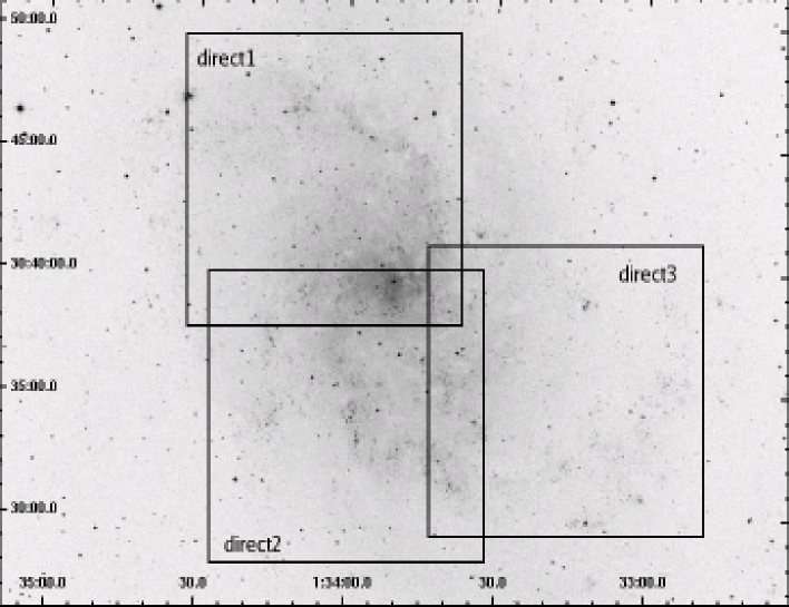
M33 central region was covered by three fields — direct1, direct2 and direct3, similar to the DIRECT three fields. Table 1 lists the fields central coordinates, and Fig. 1 shows the field boundaries on a Palomar Quick-$V$ survey image of M33.

During the three years of the project M33 was observed on 95 nights, with about 30 nights per typical observing season (In the season of 2002 – 2003 M33 was observed only on 3 nights). We made an effort to observe each of the three fields twice per observing night, although some technical and/or weather conditions did not allow all six exposures to be acquired on all nights. A total of 617 exposures were obtained and are listed on Table 2. They include 286 exposures of direct1, 177 of direct2 and 154 of direct3.

On the night of Aug. 31, 2003, at the last stage of our monitoring of M33, a nova eruption was discovered in the direct1 field (Ganeshalingam & Li, 2003). To follow-up the nova evolution, we obtained 111 exposures for the direct1 field between Sep. 7 and Sep. 22, 2003 (Shporer et al., 2003). Those images are included in our present analysis.

Table 1: Fields central coordinates (J2000.0)

Field name	RA	Dec
direct1	01:34:05.1	+30:43:43
direct2	01:34:00.0	+30:34:04
direct3	01:33:16.0	+30:35:15

Figure 1: Boundaries of the three fields over-plotted on a Palomar Quick-$V$ survey image of M33. North is up and East is to the left. Coordinates are in the J2000.0 system.

Table 2: Mid-exposure JD of all 617 $V$ exposures obtained in the course of this survey.

			direct1
1801.290	1896.308	2134.414	2181.451	2305.187	2891.514	2899.316	2900.515
1801.301	1898.196	2134.508	2181.461	2305.198	2891.525	2899.327	2900.526
⋮	⋮	⋮	⋮	⋮	⋮	⋮	⋮
			direct2
1801.324	1842.532	1927.283	2134.542	2166.489	2257.203	2301.286	2904.384
1802.297	1842.543	1931.200	2134.553	2166.500	2257.214	2301.297	2905.345
⋮	⋮	⋮	⋮	⋮	⋮	⋮	⋮
			direct3
1801.337	1829.289	1925.290	2131.554	2151.492	2259.242	2305.232	2908.536
1801.348	1829.300	1927.295	2134.457	2166.521	2259.253	2305.243	2914.344
⋮	⋮	⋮	⋮	⋮	⋮	⋮	⋮

Mid-exposure JDs are given as JD - 2450000, for each observed field separately. Only a small sample of Table 2 is presented here. The entire table is available in the MNRAS electronic issue.

2.2 Photometry

Photometric processing was performed using IRAF packages and routines. Biasing and flat field correction were done with the CCDPROC package with exposures taken nightly.

For object identification and astrometry we created for each field a reference image by combining the best 20 images. A total of 6487 objects were identified using the IRAF daofind task (Stetson, 1987). After X,Y coordinates were transformed to the coordinate system of each of the images we applied aperture photometry with the IRAF phot task in a fixed position mode. Other photometric techniques we experimented with did not result in significantly different results. Aperture radius was set to 3.5 pixels ($=2.4$ arcsec) for all images, as this value is the typical PSF FWHM.

To remove systematic effects in our data we applied the newly developed SysRem algorithm (Tamuz et al., 2005), which can remove systematic effects in large sets of photometric lightcurves. SysRem succeeded to decrease the stellar scatter of the brightest objects by up to about 50%.

Astrometry was performed using the USNO A-2.0 star catalog (Monet et al., 1998) and the reference image. CCD X,Y coordinates were transformed to equatorial FK5 with second-order polynomials. Residuals RMS were $\lesssim$ 0.45” and no single coordinate residual exceeded 1.0”.

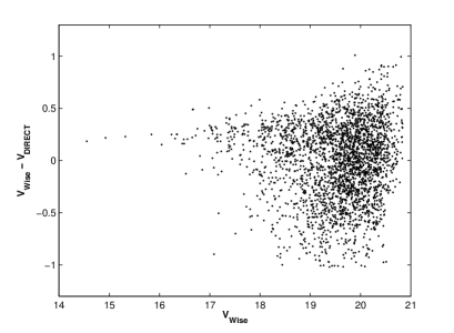
Instrumental magnitude was transformed to real magnitude using the catalog of Macri et al. (2001a). This catalog contains $V$ magnitudes of all objects observed by the DIRECT first M33 observational campaign. A linear transformation from instrumental to real magnitude was derived using objects which were successfully astrometrically matched with catalog objects, allowing a maximum distance of 2”. Fig. 2 shows the magnitude difference between Wise and DIRECT magnitude vs. Wise derived magnitude for those objects. The increased scatter in the magnitudes difference for faint stars results from the increased uncertainty in the magnitudes of those stars.

Figure 2: Difference between Wise and DIRECT magnitudes vs. Wise magnitude for astrometrically matched objects.

The RMS of the difference between Wise and DIRECT magnitudes is 0.3 – 0.4 mag, varying slightly from field to field. This scatter is similar to the scatter presented by Mochejska et al. (2001a, Figure 7, 2001b, Figure 6) and found by Lee et al. (2002).

2.3 Photometric Results and ON-Line Data

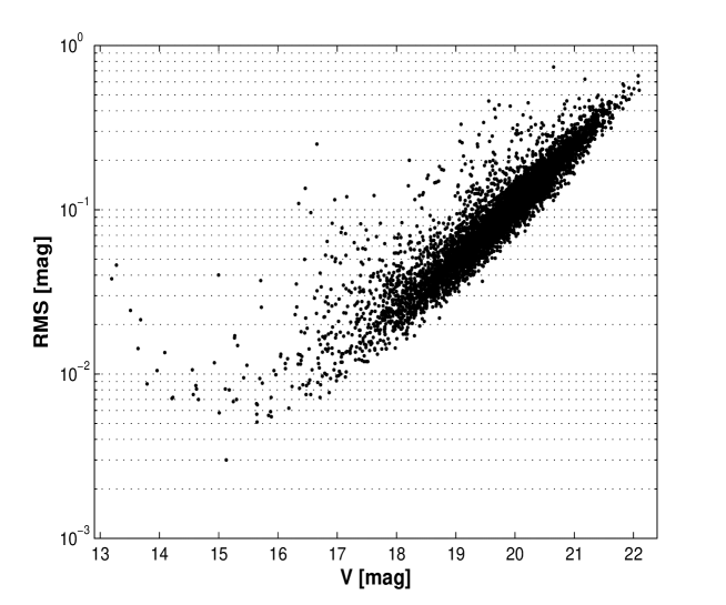
Fig. 3 presents the RMS vs. the averaged $V$ magnitude for all objects. Poisson and readout noises are dominant for objects fainter than mag $\sim\!16$. For brighter objects the scatter levels off and systematic noise at the level of $\sim\!7$ mmag becomes dominant. For stars brighter than $\sim\!14$ noise level rises again due to CCD saturation.

Table 3 lists the position, $V$ magnitude and RMS of all 6418 objects. Lightcurves, consisting of a total of 899,509 individual measurements are publicly available at the Wise Observatory FTP server at wise-ftp.tau.ac.il:/pub/shporer/m33/, which can be accessed through anonymous FTP. Each lightcurve is given as a separate text file, named ’lc’ with a 5-digit internal number extension. The listing of lc.12121 is given in Table 4.

Table 3: Object catalog

Desig.	R.A.	Dec	$V$	$\sigma$
	hh mm ss.ss	dd mm ss.s	[mag]	[mag]
W30144	01 32 55.66	30 33 02.3	20.63	0.15
W31679	01 32 55.68	30 34 27.7	18.79	0.03
W31624	01 32 55.69	30 35 34.8	17.61	0.04
W30656	01 32 55.73	30 31 41.4	19.65	0.08
W31717	01 32 55.73	30 34 30.1	18.48	0.03
W30559	01 32 55.73	30 39 31.3	20.08	0.12
W31082	01 32 55.74	30 39 22.4	20.36	0.17
W31078	01 32 55.77	30 39 12.7	19.71	0.08
W31484	01 32 55.81	30 37 13.0	16.42	0.01
W30901	01 32 55.83	30 35 24.4	19.80	0.09
⋮	⋮	⋮	⋮	⋮

Columns contain (1) designation, (2) R.A. (J2000.0), (3) Dec (J2000.0), (4) $V$ magnitude and (5) magnitude RMS. Only a small sample of Table 3 is presented here. The entire table is available in the MNRAS electronic issue.

Figure 3: RMS against real $V$ magnitude for all 6418 objects. The decrease of the Poisson noise and read noise as objects become brighter, up to a magnitude of $\sim\!16$, is the dominant feature of the diagram. For brighter objects a residual systematic noise of $\sim\!7$ mmag is observed. The increased scatter for objects brighter than $\sim\!14$th magnitude is due to CCD saturation.

Table 4: Example of an on-line lightcurve text file.

1809.4479	20.511	0.146
1809.4589	20.591	0.158
1813.5006	20.358	0.131
1819.2919	20.490	0.169
1819.3029	20.697	0.184
1819.3735	20.522	0.113
1819.3844	20.493	0.120
1820.2384	20.437	0.243
1820.2494	20.267	0.170
1820.3184	20.595	0.154
⋮	⋮	⋮

Columns contain (1) mid-exposure JD - 2450000, (2) $V$ magnitude and (3) magnitude uncertainty. Only part of the lightcurve is presented here, for guidance regarding form and content of all lightcurve text files.

3 Search for Variability

Each Lightcurve was searched first for periodic modulation, and then for non-periodic variability. For stars with available DIRECT data, we also applied periodic analysis to the combined data.

3.1 Periodicity Detection

Periodicity search was applied to all lightcurves with the Analysis of Variance (AoV) algorithm of Schwarzenberg-Czerny (1989). For each trial frequency, $\nu$, data was folded with the corresponding period and then binned into 10 bins, using equal as possible number of points per bin. Two variances were calculated: Binned lightcurve variance, $s_{1}^{2}(\nu)$, and the sum of bins internal variance, $s_{2}^{2}(\nu)$. Periodogram value, $S(\nu)$, was taken as the ratio of those variances, $s_{1}^{2}(\nu)/s_{2}^{2}(\nu)$.

For each lightcurve, we defined $\mathcal{S}$ as the value of the highest periodogram peak divided by periodogram average:

$$\mathcal{S}=\frac{max_{\nu}S(\nu)}{<S(\nu)>_{\nu}}\,.$$ (1)

We consider the value of $\mathcal{S}$ as an indicator of the significance of the detection of a periodicity within the lightcurve.

To estimate the significance of the periodicity detection we computed $\mathcal{S}$ for 100 random permutations of every lightcurve in each of the three fields, obtaining an $\mathcal{S}$ distribution consisting of $\sim 2\times 10^{5}$ elements per field. We defined $\mathcal{H}_{S}(S)$ to be the percentage of randomly permuted lightcurves with higher $\mathcal{S}$ values. Stars with $\mathcal{H}_{S}(S)$ smaller than $0.01\%$ were flagged as periodic. This threshold gives an expectation of one false detection for every $10^{4}$ lightcurves, or, $0.64$ for our entire sample.

A total of 113 periodic variables were detected. The period uncertainty, ${\Delta}P$, was defined as the FWHM of the periodogram peak. In order to derive the amplitude we applied an iterative running-median to the phased lightcurve and took half the magnitude difference between maximum and minimum brightness.

We have classified 45 periodic variables as Cepheids by examining the period, amplitude and shape of all periodic variables. In particular, we examined the relative duration of increasing and decreasing brightness, in order to detect stars with an increasing phase substantially shorter than the decreasing phase. Comparing with the publicly available DIRECT catalogs and the SIMBAD astronomical database we find that 8 out of the 45 Cepheids are new, and 37 are previously known Cepheids. The 8 new Cepheids are listed in Table 5 and plotted in Fig. 4. Five of the new Cepheids were not identified before as variables, and the other 3 were classified as variables and had no known period. The 5 new Cepheids are positioned in our direct3 field and in the DIRECT M33C field. Variables of this field were not reported by the DIRECT project, although Table 9 of Macri et al. (2001b, reporting variables in fields M33A and M33B) includes 15 M33C variables. (The 37 known Cepheids are included in Table 11 which lists all variables identified here.)

Table 5: List of 8 new Cepheids. Five of the new Cepheids were not identified before as variables and the other 3 were classified as variables and had no known period.

Desig.	R.A.	Dec.	$V$	$\sigma$	Amp.	Period	${\Delta}P$	Comments
	hh mm ss.ss	dd mm ss.s	[mag]	[mag]	[mag]	[days]	[days]
New Variables
W30837	1 33 27.66	30 34 24.0	19.52	0.12	0.15	14.837	0.073	1
W31339	1 32 57.55	30 38 46.5	19.36	0.15	0.16	18.553	0.096	1
W31573	1 33 16.45	30 36 58.2	19.65	0.15	0.18	18.553	0.091	1
W31027	1 33 30.15	30 38 04.8	20.45	0.34	0.35	19.920	0.100	1
W30348	1 33 30.40	30 35 55.8	19.67	0.36	0.45	22.08	0.13	1
New Periodic Variables
W22288	1 33 57.56	30 38 44.8	18.04	0.07	0.08	26.74	0.16
W20128	1 34 15.47	30 31 06.7	18.93	0.08	0.10	28.01	0.17
W21681	1 33 39.92	30 35 08.2	18.31	0.12	0.15	51.28	0.91

Columns contain (1) Designation, (2) J2000.0 R.A., (3) J2000.0 Dec., (4) mean $V$ magnitude, (5) magnitude RMS, (6) amplitude, (7) period, (8) period uncertainty and (9) comments.

Comments: 1: Position in DIRECT M33C field.

Figure 4: Lightcurves of the 8 new Cepheids detected here. Magnitude is plotted against phase. Title of each lightcurve is composed of (from left to right) designation, period, in days, and mean $V$ magnitude.

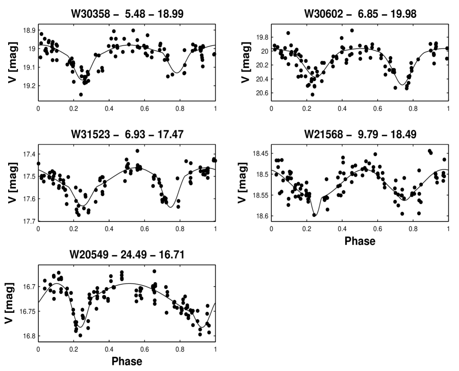
In order to detect EBs we applied the Eclipsing Binary Automated Solver (Tamuz, Mazeh & North 2006, Mazeh, Tamuz & North 2006, hereafter EBAS) to all periodic variables that were not identified as Cepheids. EBAS has its own built in goodness-of-fit estimator, the alarm — $\mathcal{A}$, which we used to identify the true EBs. The advantage of the alarm over the classical $\chi^{2}$, as a goodness-of-fit estimator, results from accounting for measurements order, by considering maximal series of consecutive, mean-subtracted measurements with the same sign. We manually inspected all objects with $\mathcal{A}$ $<1.0$, in order to remove spurious EB classifications. We identified 12 systems as EBs, of which 5 are new, presented in Fig. 5 and listed in Table 6. Those 5 include four new variables and one new classification of a known, unclassified periodic object (W21568). Table 3.1 lists the EBAS solution parameters of all 12 EBs detected here. The 7 already known EBs are included in Table 11.

Table 6: List of 5 new eclipsing-binaries. Three of those were not identified before as variables, and the other one was identified as an unclassified periodic.

Desig.	R.A.	Dec.	$V$	$\sigma$	Comments
	hh mm ss.ss	dd mm ss.s	[mag]	[mag]
New Variables
W30358	1 32 57.31	30 36 07.6	19.04	0.07	1
W31523	1 33 29.88	30 31 47.5	17.52	0.07	1
W30602	1 33 35.31	30 40 24.7	20.15	0.19	1
W20549	1 33 58.67	30 35 26.6	16.73	0.03
New Classification
W21568	1 33 54.80	30 32 49.0	18.52	0.04

Columns contain (1) Designation, (2) J2000.0 R.A., (3) J2000.0 Dec., (4) mean $V$ magnitude, (5) magnitude RMS and (6) comments.

Comments: 1: Position in DIRECT M33C field.

Table 7: EBAS orbital solutions for the 12 eclipsing-binaries identified here.

Desig.	$\mathcal{A}$	$V$	Period	$r_{t}$	$k$	$J_{s}$	$x$	$e\,cos\,w$	$e\,sin\,w$	$A_{p}$	$A_{s}$
		[mag]	[days]
W21612	-0.09	19.4681	2.337324	0.706	0.2	1.9	0.79	0.014	-0.018	0.995	1.0000
		$\pm$3.2e-02	$\pm$8.5e-05	$\pm$9.7e-02	$\pm$1.2e+00	$\pm$2.6e+00	$\pm$1.3e-01	$\pm$3.1e-02	$\pm$4.4e-02	$\pm$2.6e-02	$\pm$2.3e-03
W11486	0.12	18.359	2.70811	0.81	0.93	0.75	0.800	0.034	-0.037	0.99	1.000
		$\pm$3.1e-02	$\pm$1.1e-04	$\pm$1.0e-01	$\pm$5.8e-01	$\pm$2.7e-01	$\pm$8.1e-02	$\pm$2.4e-02	$\pm$4.5e-02	$\pm$2.1e-01	$\pm$1.4e-02
W11491	-0.22	18.980	3.84684	0.640	1.44	1.27	0.64	0.002	0.08	1.0000	1.00
		$\pm$7.2e-02	$\pm$3.2e-04	$\pm$9.7e-02	$\pm$8.0e-01	$\pm$8.4e-01	$\pm$1.1e-01	$\pm$4.7e-02	$\pm$1.0e-01	$\pm$3.9e-03	$\pm$1.7e-01
W10764	0.55	20.318	4.432920	0.731	0.59	1.43	-0.09	-0.060	0.05	0.016	0.08
		$\pm$7.0e-02	$\pm$7.1e-05	$\pm$5.7e-02	$\pm$5.6e-01	$\pm$6.0e-01	$\pm$1.3e-01	$\pm$2.3e-02	$\pm$1.0e-01	$\pm$1.3e-02	$\pm$1.6e-01
W20942	0.53	20.739	5.09566	0.670	1.06	0.67	-0.001	-0.015	-0.06	1.0000	0.34
		$\pm$4.9e-02	$\pm$1.6e-04	$\pm$6.8e-02	$\pm$2.3e-01	$\pm$1.9e-01	$\pm$8.5e-02	$\pm$2.5e-02	$\pm$1.2e-01	$\pm$9.2e-03	$\pm$2.6e-01
W30358	0.16	18.990	5.48325	0.634	0.68	1.36	0.661	0.047	0.061	0.000	1.000
		$\pm$3.7e-02	$\pm$3.3e-04	$\pm$3.7e-02	$\pm$4.4e-01	$\pm$4.7e-01	$\pm$5.2e-02	$\pm$1.2e-02	$\pm$5.6e-02	$\pm$3.9e-02	$\pm$1.6e-03
W30051	0.78	18.5282	6.624649	0.6751	2.64	0.67	-0.015	-0.0645	0.024	0.07	1.00
		$\pm$7.3e-03	$\pm$1.1e-05	$\pm$9.7e-03	$\pm$9.0e-01	$\pm$1.2e-01	$\pm$5.1e-02	$\pm$5.4e-03	$\pm$1.4e-02	$\pm$2.0e-01	$\pm$1.4e-01
W30602	-0.16	19.980	6.85114	0.785	0.93	0.99	0.41	-0.017	-0.106	1.00	0.00
		$\pm$6.6e-02	$\pm$4.1e-04	$\pm$6.1e-02	$\pm$5.1e-01	$\pm$1.6e-01	$\pm$1.0e-01	$\pm$1.7e-02	$\pm$9.7e-02	$\pm$2.8e-01	$\pm$2.6e-01
W31523	-0.18	17.473	6.92557	0.634	1.71	0.73	0.784	-0.0056	-0.106	0.005	1.000
		$\pm$1.6e-02	$\pm$1.2e-04	$\pm$3.3e-02	$\pm$4.0e-01	$\pm$6.6e-02	$\pm$1.7e-02	$\pm$5.4e-03	$\pm$1.6e-02	$\pm$3.4e-02	$\pm$5.7e-02
W22214	-0.23	18.582	8.77401	0.455	3.8	0.89	0.32	-0.031	-0.001	0.902	0.99983
		$\pm$2.4e-02	$\pm$4.1e-04	$\pm$1.5e-02	$\pm$1.3e+00	$\pm$3.7e-01	$\pm$1.7e-01	$\pm$1.0e-02	$\pm$3.9e-02	$\pm$2.6e-02	$\pm$1.5e-04
W21568	-0.20	18.493	9.7870	0.549	4.0	0.050	0.947	0.002	-0.067	1.000	0.13
		$\pm$2.9e-02	$\pm$1.3e-03	$\pm$3.9e-02	$\pm$1.1e+00	$\pm$7.2e-02	$\pm$5.4e-02	$\pm$3.1e-02	$\pm$3.7e-02	$\pm$3.3e-02	$\pm$2.2e-01
W20549	0.27	16.71	24.4920	0.652	1.16	1.343	0.7938	0.2464	0.0600	0.940	0.36
		$\pm$1.1e-1	$\pm$3.9e-3	$\pm$2.1e-2	$\pm$1.1e-1	$\pm$5.2e-2	$\pm$9.2e-3	$\pm$6.7e-3	$\pm$8.1e-3	$\pm$6.1e-2	$\pm$1.0e-1

Columns contain (1) Designation, (2) alarm, (3) out-of-eclipse $V$ magnitude, (4) period, in days, (5) relative sum of radii, (6) radii ratio, (7) surface brightness ratio, (8) impact parameter, (9) eccentricity, $e$, multiplied by cos$w$ and (10) by sin$w$, where $w$ is the periastron longitude, (11) bolometric reflection coefficient for the primary binary component and (12) for the secondary component.

Figure 5: Lightcurves of the 5 new EBs detected here. Magnitude is plotted against phase. EBAS lightcurve solution is presented by a solid line. Title of each lightcurve is composed of (from left to right) Designation, EBAS period, in days, and EBAS out-of-eclipse $V$ magnitude.

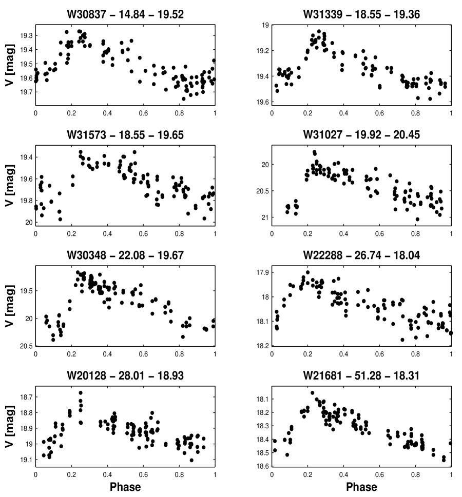
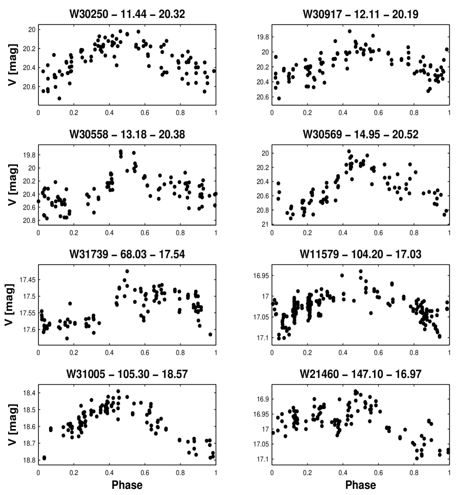
Periodic variables not identified as Cepheids or EBs were noted as unclassified periodic. Those include 56 objects, 26 of which were not known before as periodic variables, listed on Table 8. (The 30 known periodic variables are included in Table 11.) The 26 new unclassified periodics include 19 new variables (not known before as variables) and 7 previously known as non-periodic variables. A sample of 8 new unclassified periodic variables is presented in Fig. 6.

In addition, we have determined an improved period, of 175.4 days, for W11984 where the previously known period was 458 days (Kinman et al., 1987).

Table 8: List of 26 new unclassified periodic variables. Twenty of those were not identified before as variables. The other 8 are known variables without a known period.

Desig.	R.A.	Dec.	$V$	$\sigma$	Amp.	Period		${\Delta}P$		Comments
	hh mm ss.ss	dd mm ss.s	[mag]	[mag]	[mag]	[days]		[days]
New Variables
W10109	1 34 15.57	30 41 10.1	18.61	0.04	0.04	9.	718	0.	021
W30344	1 33 27.37	30 35 51.5	20.81	0.24	0.25	11.	211	0.	021	1
W30250	1 33 25.58	30 34 27.0	20.32	0.18	0.19	11.	442	0.	047	1
W30917	1 33 18.48	30 35 34.3	20.19	0.18	0.18	12.	107	0.	061	1
W30558	1 33 31.65	30 39 32.0	20.38	0.26	0.27	13.	175	0.	048	1
W30569	1 33 32.17	30 39 46.2	20.52	0.29	0.33	14.	948	0.	046	1
W20380	1 34 16.05	30 33 44.9	16.79	0.02	0.03	15.	773	0.	063
W12052	1 34 00.90	30 40 25.1	18.25	0.04	0.05	26.	46	0.	34
W12073	1 33 45.15	30 44 19.0	18.02	0.04	0.04	52.	9	1.	2
W31739	1 33 12.34	30 38 48.7	17.54	0.05	0.05	68.	03	0.	80	1
W31230	1 33 11.16	30 34 21.9	16.80	0.03	0.04	99.	3	4.	4
W11579	1 33 48.32	30 42 41.4	17.03	0.03	0.03	104.	2	3.	1
W31005	1 33 05.77	30 37 20.3	18.57	0.09	0.15	105.	3	3.	4	1
W31047	1 33 15.76	30 38 22.1	17.96	0.05	0.07	117.	6	3.	8	1
W30803	1 33 00.09	30 33 41.4	19.27	0.10	0.09	140.	8	4.	8	1
W21460	1 33 50.96	30 38 19.4	16.97	0.05	0.08	147.	1	5.	0
W30292	1 32 59.34	30 35 05.1	17.91	0.04	0.04	222		13		1
W11898	1 34 10.91	30 41 41.6	18.70	0.05	0.06	270		34
W31416	1 33 12.60	30 32 52.5	19.51	0.20	0.31	278		29		1
New Periodic Variables
W30043	1 33 36.60	30 31 55.0	19.36	0.09	0.09	13.	624	0.	068
W21058	1 33 41.34	30 32 12.9	18.24	0.06	0.06	20.	12	0.	16
W21193	1 33 58.33	30 34 29.7	18.04	0.04	0.04	36.	50	0.	29
W21387	1 34 05.42	30 37 19.7	19.16	0.10	0.13	135.	1	6.	5
W20509	1 33 55.58	30 35 01.0	17.39	0.04	0.06	144.	9	7.	0
W11870	1 33 52.39	30 39 08.4	16.55	0.10	0.15	263		10
W10678	1 33 58.93	30 41 38.5	17.11	0.02	0.04	286		26

Columns contain (1) Designation, (2) J2000.0 R.A., (3) J2000.0 Dec., (4) mean $V$ magnitude, (5) magnitude RMS, (6) period, (7) period uncertainty ,(8) amplitude and (9) comments.

Comments: 1: Position in DIRECT M33C field.

Figure 6: Lightcurves of eight new unclassified periodics, out of the 26 new periodic variables identified here. Magnitude is plotted against phase. Title of each lightcurve is composed of (from left to right) designation, period, in days, and mean $V$ magnitude.

3.2 Non-Periodic Variability Detection

All non-periodic lightcurves were searched for variability using the alarm statistic, $\mathcal{A}$, introduced by Tamuz et al. (2006). Here, the alarm is used to detect variable lightcurves by estimating the goodness-of-fit of a constant function. The significance of the detection of the variability was estimated by a permutation test, as was done for the periodicity detection. For each single lightcurve, we generated $10^{5}$ random permutations and calculated their alarm value. For each real lightcurve we defined $\mathcal{H}_{A}(A)$ to be the percentage of randomly permuted lightcurves with higher $\mathcal{A}$ values. Lightcurves with $\mathcal{H}_{A}(A)$ smaller than $0.01\%$ were flagged as non-periodic variables.

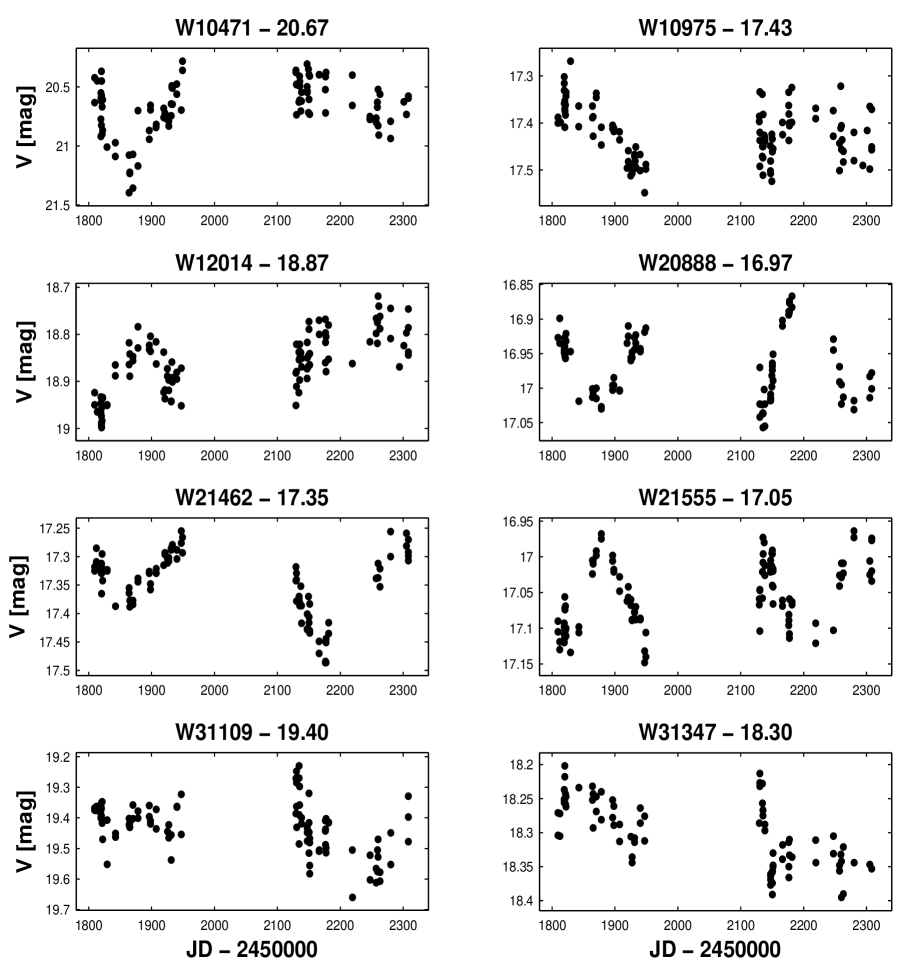
A total of 177 non-periodic variables were detected. Those include 99 new variables, listed on Table 9. (The 78 previously known are included in Table 11.) A sample of eight new non-periodic variables is presented on Fig. 7.

Figure 7: Lightcurves of eight new non periodic variables, out of the 99 new non-periodics detected here. Magnitude is plotted vs. JD - 2450000. Title of each lightcurve is composed of (from left to right) designation and mean $V$ magnitude. Data of only the first two observational seasons is presented on the above plots, to make the variability more apparent.

Table 9: List of 99 new non-periodic variables.

Desig.	R.A.	Dec.	$V$	$\sigma$	Comments
	hh mm ss.ss	dd mm ss.s	[mag]	[mag]
W31624	1 32 55.69	30 35 34.8	17.61	0.04	1
W31074	1 32 56.73	30 39 04.0	19.22	0.12	1
W31279	1 32 57.86	30 35 55.1	19.13	0.10	1
W30354	1 32 58.19	30 36 06.4	18.80	0.17	1
W31223	1 32 59.58	30 34 05.8	19.23	0.08	1
W30648	1 32 59.70	30 31 37.0	19.84	0.12	1
W31070	1 32 59.74	30 38 55.1	18.06	0.06	1
W30214	1 33 00.94	30 34 04.0	19.19	0.08	1
W30877	1 33 01.02	30 35 00.7	18.79	0.08	1
W30185	1 33 01.70	30 33 29.6	19.55	0.10	1
⋮	⋮	⋮	⋮	⋮	⋮

Columns contain (1) Designation, (2) J2000.0 R.A., (3) J2000.0 Dec., (4) mean $V$ magnitude, (5) magnitude RMS and (6) Comments.

Comments: 1: Position in DIRECT M33C field. 2: Position outside all three DIRECT fields.

Only a small sample of Table 9 is presented here. The entire table is available in the MNRAS electronic issue.

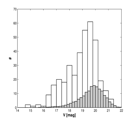
Fig. 8 presents a mean $V$ magnitude histogram of all variable (periodic and non-periodic) objects detected here, indicating a completeness magnitude of about 19.5. For comparison, the corresponding histogram for all objects, where bin hight was reduced by a factor of 40, is also presented, in gray.

Figure 8: Magnitude histogram of all variables detected here, showing a completeness magnitude of about 19.5. Corresponding (scaled) histogram for all objects is presented in gray.

3.3 Combined Lightcurves

We combined the data presented in this paper with the available data for DIRECT variables from Macri et al. (2001a) and Mochejska et al. (2001a, b). Data from all three sources were combined to create $\la$ 7 years time span lightcurves, although with large gaps, of up to 500 $V$ measurements each. Combining data from several telescopes requires fine calibration, removing possible zero point differences, when searching for variables in particular.

To derive a periodogram we fitted the data from the three telescopes with a few harmonics for each frequency together with different zero points for the three data sources. Those zero points were fitted separately for each variable. Since there is a large scatter in the magnitude difference of the same stars in different telescopes (See Fig. 2 and Mochejska et al. (2001a, Figure 7, 2001b, Figure 6)) taking the same zero point shift for all lightcurves would not be accurate enough.

Periodogram value for each frequency was taken to be the fitted amplitude divided by the ${\chi}^{2}$ goodness-of-fit parameter. We then divided the whole periodogram by a fitted polynomial, using a cubic smoothing spline fit. Number of harmonics used for each frequency in the fit was determined by using the Akaike Information Criterion (AIC, Akaike, 1974). Fig. 3.1 shows an example of this analysis for W10821.

Figure 9: Combined lightcurve analysis of W10821 and its DIRECT counterpart — D33J013343.4+304356.5. Two harmonics were fitted to 462 measurements (of a time span of 2615 days). Top panel shows data of the DIRECT 1st campaign (Macri et al., 2001b), in circles, of the DIRECT 2nd campaign (Mochejska et al., 2001a), in crosses, and data obtained here, in triangles. Middle panel presents the periodogram where the 2nd strongest frequency is consistent with one half the strongest frequency value, respectively. Bottom panel shows the combined phase-folded lightcurve, where the fitted zero point of each data set was subtracted. Fitted zero points are 19.43, 19.91 and 19.90 mag for the DIRECT 1st campaign (Macri et al. 2001b, marked by circles), DIRECT 2nd campaign (Mochejska et al. 2001a, marked by crosses) and the Wise data (marked by triangles), respectively. The black solid line is just an harmonic fit, derived by the lightcurves combining procedure.

Lightcurves of 59 periodic objects were combined with data obtained here. For 9 of those stars results were unsatisfactory, mainly due to high noise level of faint objects. Results of the combining analysis for 50 objects are presented on Table LABEL:table:comb_lc, together with the periods obtained previously by the two DIRECT project programs.

Columns contain (1) Wise Designation, (2) period of Macri et al. (2001b), (3) period of Mochejska et al. (2001a, b), (4) period of the combined lightcurves, (5) Period uncertainty, (6) amplitude of the fit, (7) zero point shift of Mochejska et al. (2001a, b) relative to Macri et al. (2001b), and (8) zero point shift of the Wise data relative to Macri et al. (2001b).

Except for two objects, W10034 & W20923, period derived by the combining procedure is consistent with those derived by analyzing each data set separately. For W10034, analysis of the combined lightcurve was able to reveal the true period (107.53 days), which is twice the period derived previously. For W20923, we have detected a period of 69.44 days, while the DIRECT period is 56.84. It is also interesting to note that a period of 69.50 days was already derived by Hubble (1926, Table II, variable No. 10) for this object.

Figure 10: Combined lightcurve of W10034 with its DIRECT counterpart — D33J013420.8+303943.0, revealing the true period of 107.53 days, twice then period derived previously. Only by analyzing the combined lightcurve, consisting of 490 measurements taken in a time span of 2608 days, the true period was derived. The different markings for each data set are the same as in Fig. 3.1, bottom panel.

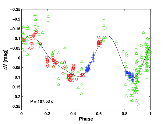
Table 11 lists all variables detected here along with designation of known variables.

Table 11: List of all 290 variables detected in this survey. Within each variability type objects are sorted by increasing period and the non-periodic variables are sorted by increasing R.A. For previously known variables their known designation is given.

Wise						Known
Desig.	R.A.	Dec.	Type	Period		Designation	Type	Period	Comments
	hh mm ss.ss	dd mm ss.s		[days]				[days]
W21612	01 33 56.26	+30 33 58.8	E	2.337324		D33J013356.2+303358.6	E	2.34
W11486	01 33 54.32	+30 40 28.9	E	2.70811		D33J013354.3+304029.6	E	2.71
W11572	01 33 45.93	+30 42 30.3	C	12.9199		D33J013346.0+304231.9	C	12.93	10
W10128	01 34 02.76	+30 41 44.4	C	13.0634		D33J013402.8+304145.7	C	13.04	10
W21162	01 33 60.96	+30 33 54.8	P	2.1142		D33J013359.8+303354.9	P	2.12
W21067	01 33 41.63	+30 32 20.5	P	5.2618		D33J013341.6+303220.3	P	5.30	10
W31624	01 32 55.69	+30 35 34.8	N	-		-	-	-	1,4
W31074	01 32 56.73	+30 39 04.0	N	-		-	-	-	1,4
⋮	⋮	⋮	⋮	⋮		⋮	⋮	⋮	⋮

Key to variability types: E — Eclipsing binary, C — Cepheid, P — Unclassified Periodic, N — Non-periodic variable (DIRECT miscellaneous type).

Comments: 1: New variable; 2: New classification of a known variable; 3: Position in DIRECT M33C, reported in Table 9 of Macri et al. (2001b); 4: Position in DIRECT M33C (new variable); 5: Position outside all DIRECT fields (new variable); 6: Object detected as periodic variable by Shemmer et al. (2000); 7: Astrometric matching between Wise and DIRECT objects can not be determined accurately due to the crowded region; 8: classified as a Long Period Variable (LPV) by Kinman, Mould & Wood (1987); 9: Object detected as variable by Hubble & Sandage (1953); 10: Period derived from the combined lightcurve.

Only a small sample of Table 11 is presented here, including two objects from each variability type. The entire table is available in the MNRAS electronic issue.

3.4 Comparison with the DIRECT results

Table 12: Summary of the detections by the Wise Observatory

Var. Type	All Fields	M33A & M33B		M33C		Out	Previous	New Class.	New Var.
		Wise	DIR	Wise	DIR
Cepheid	45	34	34	11	6	-	-	3a	5
EB	12	8	7	4	1	-	-	1b	4
Unclass. Per.	56	40	34	16	1	-	2	7a	19
Non Per.	177	136	73	38	2	3	3	-	99
Total	290	218	148	69	10	3	5	11	127

Columns contain: (1) variability type and (2) number of detected variables. (3) Variables detected here inside the DIRECT M33A and M33B fields and (4) of those, number of variables detected by the DIRECT, including objects for which a new variability class was obtained here. (5) Variables detected here inside the DIRECT M33C field and (6) of those, number of variables detected by the DIRECT (Macri et al. 2001b, Table 9). Only variables in M33C and not in overlapping regions are listed on columns 5 and 6. (7) Variables detected outside the DIRECT FOVs. (8) Variables detected here, detected previously by studies other than the DIRECT. (Hubble & Sandage 1953, Kinman et al. 1987 and Shemmer et al. 2000). (9) Newly classified variables and (10) new variables.

Notes: (a) classified by DIRECT as non-periodic. (b) classified by DIRECT as an unclassified periodic.

Many objects classified here as variables were not classified as such by the DIRECT project. Out of the total 290 variables detected here only 158 variable objects were astrometrically matched to DIRECT variables. The other 132 variables consist of 102 non-periodic and 30 periodic variables. Of those 132, 5 were already identified as variables by previous studies (Hubble & Sandage 1953, Kinman et al. 1987 and Shemmer et al. 2000), giving a total of 127 new variables, consisting of 99 non-periodic and 28 periodic. In addition, we obtained an improved variability type for 11 of the 158 astrometrically matched variables.

The M33 area monitored here includes three fields, while the DIRECT catalogs of Macri et al. (2001b) and Mochejska et al. (2001a, b) list variables from only two fields, M33A and M33B. Those fields are also slightly smaller than the corresponding direct1 and direct2 fields observed here. Considering only the 221 variables we find here inside the FOV of DIRECT M33A and M33B fields, 148 of them are present in the variables catalogs of Macri et al. (2001b) or Mochejska et al. (2001a, b). The other 73 variable objects include 63 non-periodic and 10 periodic variables.

Table 12 lists the number of variables detected here, of each variability type, and of those, number of variables detected by the DIRECT project. Table 12 also refers to variables positioned in the DIRECT M33C field since although this field’s variables were not reported by the DIRECT, 15 of them are included in Table 9 of Macri et al. (2001b). Also given in Table 12 are number of variables detected outside all three DIRECT fields, variables detected by other, previous studies, number of newly classified variables and of new variables.

4 Interesting Variables

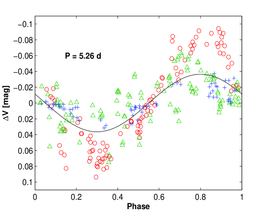
4.1 W21067 — An Optical Periodic X-Ray Source

The combined data of W21067 (1:33:41.63, +30:32:20.5), one of the brightest objects in the sample, yielded a period of 5.26 days with an amplitude of 0.04 (see Fig. 11). An X-ray source at a distance of 1.4” from our position of W21067 was detected by Pietsch et al. (2004, Table 3, source 194) using the XMM-Newton observatory. They have measured an 0.2–4.5 KeV flux of $(1.3900\pm 0.0097)\times 10^{-14}$ erg/sec/cm² and also suggested that the positional correlation between an optically periodic variable and an X-ray source makes this object an XRB candidate.

Figure 11: Combined lightcurve of W21067 folded on the period detected by the combining procedure, of 5.2618 days. Data of DIRECT 1st campaign (Macri et al., 2001b) is marked in circles, of DIRECT 2nd campaign (Mochejska et al., 2001b) in crosses and data obtained here in triangles. The solid line is a single harmonic fit calculated by the combining procedure (See section 3.3).

To follow this suggestion Alceste Bonanos of the CfA obtained for us a multi-order spectrum of W21067 with the Echellette Spectrograph and Imager (ESI) at the Keck II 10-m telescope in the Echelle mode. Fig. 12 presents the joined spectrum of all 10 orders (orders 6 to 15), with a complete spectral coverage from 3900–10000 Å . Velocity dispersion is about 11.4 km/sec/pixel in all orders.

Figure 12: Joined spectrum from all 10 orders of W21067, taken by the Keck II ESI. Normalized flux is plotted against wavelength. Spectrum was smoothed using a running mean of 5 adjacent pixels.

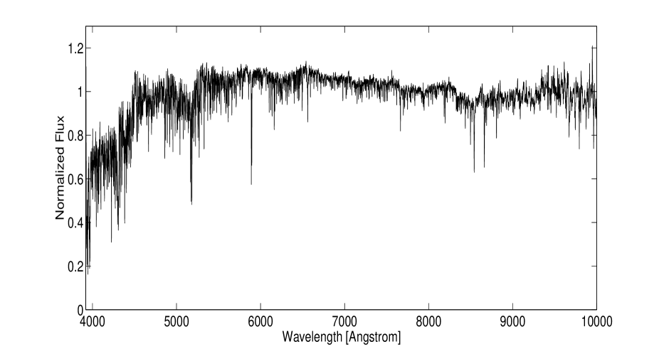
By correlating W21067’s spectrum with the ELODIE library of template spectra we were able to determine it is a K star, with a heliocentric radial velocity of $+16.4\pm 0.6$ km/s. The derived velocity is significantly different from the systemic radial velocity of M33, of $-179\pm 3$ km/s (de Vaucouleurs et al., 1991). The most plausible conclusion therefore is that W21067 is not an M33 member but a Galactic foreground object.

The many absorption lines and absence of significant emission features in W21067 spectrum rules out the possibility of a compact binary companion as the X-rays source (Bradt & McClintock, 1983). Therefore we propose chromospheric activity as the source of the optical periodicity and X-ray radiation.

The periodic modulations of chromospherically active stars are known to show long-term amplitude and shape variations, resulting from their dark regions evolution during solar-like activity cycles (Guinan & Giménez 1992, Oláh et al. 2000, Rodono 1992). This might be the cause for the somewhat large scatter in W21067 combined folded lightcurve, consisting of data from a period of $\sim$7 years.

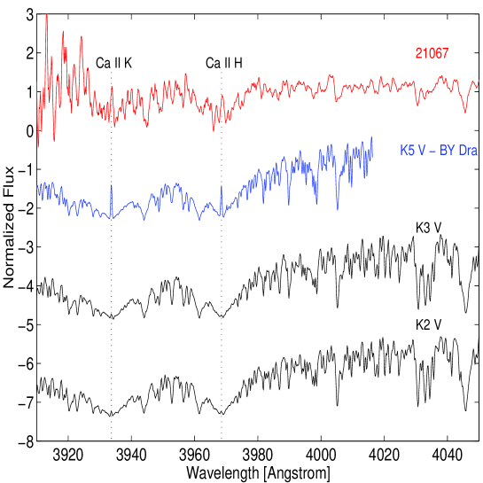
Fill-in cores of the Ca II H & K absorption lines, at 3968.5 Å and 3933.7 Å , respectively, are a classical spectral feature used to identify chromospheric activity (Fekel & Balachandran 1993, Strassmeier et al. 1993). Fig. 13 shows W21067 Ca II H & K lines together with an active star and two inactive stars of a similar spectral type. Despite the decreased S/N close to the spectrum’s blue end caused by the lower CCD QE and increased atmospheric extinction at these wavelengths, fill-in cores of W21067 Ca II H & K lines can be noticed.

The color-temperature color-index relation (Allen, 1973) for the DIRECT $B-V=0.79~{}\pm~{}0.04$ color index yields a color temperature of  $T_{c}~{}=~{}5250~{}\pm~{}150^{\,\,{}^{\circ}}$K. For Galactic object in the direction of M33 extinction and reddening can be neglected, and therefore we can assume the temperature estimate is valid. The effective temperature bolometric correction (BC) relation (Allen, 1973) yields $BC~{}=~{}0.18~{}\pm~{}0.03$ mag, which results in an X-ray to $V$ flux ratio of $log(f_{X}/f_{V})~{}=~{}-2.72\pm 0.04$, consistent with the mean value of $-2.9~{}\pm~{}0.8$ (median $-2.8$), given by Padmakar et al. (2000) for 202 active binaries.

Figure 13: From top to bottom: Spectrum of W21067 at the Ca II H & K spectral region. Spectrum of a chromospherically active star, HD 201091, a BY Dra K5 V star. Spectra of two inactive stars for comparison (HD 4628 K2 V, HD 16160 K3 V). Spectra of comparison stars were taken from Montes et al. (1997).

4.2 W31230 — An Optical Periodic at SNR Position

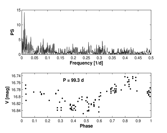
W31230 (1:33:11.17, 30:34:21.9) is located 0.41” from SNR 19 of Gordon et al. (1998) and was detected here as an unclassified periodic variable. Considering the number of SNRs and periodic variables detected here in the direct3 field, the probability of a random positional correlation is 0.0009. Calzetti et al. (1995) list this object as an $H_{\alpha}$ emitter and Sholukhova et al. (1999) detected an $H_{\alpha}$ emitter at a distance of 2.2” from W31230, for which they measured an $H_{\alpha}$ equivalent width of 19 Å. W31230 is located at the DIRECT M33C field and was not reported as variable by them. Our analysis detected a period of $99.3\pm 4.4$ days and an amplitude of 0.04 mag. Fig. 14 presents a Lomb-Scargle (Scargle, 1982) power spectrum and a phased lightcurve of our data for this star.

Figure 14: Top panel presents a Lomb-Scargle power spectrum of W31230 (normalized to unit mean) and the bottom panel shows the phased lightcurve, with an amplitude of 0.04 mag.

4.3 Optical Variables at Wolf-Rayet Positions

WR Variability can originate from random winds variations, rotation, spots evolution and pulsation, radial and non-radial (Moffat & Shara, 1986). A persistent periodic variability might indicate a WR in a binary system where variability is induced by either geometric eclipses, wind eclipses or proximity effects (Marchenko et al., 1998).

By correlating our variables against the SIMBAD database we found two objects which are located at positions of WR stars and a third object located at the position of a WR candidate. All three astrometric matches are within 1.1”.

W20549 (1:33:58.67, 30:35:26.6), a spectroscopically confirmed M33 WR (Massey & Johnson, 1998, WR115) of type WNE (Massey et al., 1995), was identified here as a new EB, with a period of 24.4920 days and orbital eccentricity of 0.25 (see Fig. 5 and Tables 6 & 3.1). W31347 (1:33:27.25, 30:39:09.7), a spectroscopically confirmed M33 WR of type WN9 (Massey & Johnson, 1998, WR39), was detected as a new non-periodic variable (see Fig. 7 and Table 9). W10975 (1:34:20.30, 30:45:45.4) was identified as a WR candidate by Massey et al. (1987, Table 2, object 29) and was detected here as a new non-periodic variable (see Fig. 7 and Table 9).

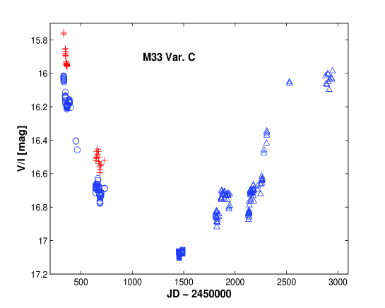
4.4 W31284 - M33 Variable C

W31284 (1:33:35.13, 30:36:00.8) is a known LBV, named M33 Variable C, discovered by Hubble & Sandage (1953, Fig. 6) by using data from 1921 to 1953. Since then, this star was included in a few other long-term surveys: Rosino & Bianchini (1973, Fig. 8), from 1960–1972, Kinman et al. (1987, Fig. 5) from 1982–1985 and Kurtev et al. (1999, Fig. 2) from 1982–1990.

In both DIRECT campaigns and in this work M33 Var. C was identified as a non-periodic variable. Lightcurve containing data of the three telescopes, with a time span of 7.16 years, is presented on Fig. 15. Although there might be small zero-point shifts between telescopes, a decrease of more than 1 magnitude, followed by a similar increase is evident. This lightcurve and the one presented by Kinman et al. (1987), show brightness variations with a much shorter time-scale than observed by Hubble & Sandage (1953) and Rosino & Bianchini (1973). Furthermore, Fig. 15 shows that the star stayed at minimum brightness for a relatively short time before brightening again, a behavior which was not observed previously. This suggests that M33 Var. C brightness variations became more rapid since the 1980s.

Figure 15: M33 Var. C lightcurve from DIRECT and this work. $V$-band data of the DIRECT first campaign is presented in circles, of the DIRECT second campaign in squares and from this work in triangles. DIRECT first campaign $I$-band data is marked by crosses. $V$-band lightcurve shows a decrease of about 1 magnitude in the star’s luminosity followed immediately by a similar increase. Variability time-scale is shorter than observed by Hubble & Sandage (1953) and Rosino and Bianchini (1973).

4.5 W11324 - LBV Periodic Microvariability Confirmation

W11324 (1:34:06.59, 30:41:46.8) is known as B416 (Humphreys & Sandage, 1980). It was identified by Shemmer, Leibowitz & Szkody (2000, hereafter SLS) as an LBV, confirming Massey et al. (1996) LBV candidate classification. SLS also report a periodic microvariability of 8.26 days with a $V$ amplitude of 27 mmag, a $V$ magnitude of 16.7$\pm$0.1 and an $H_{\alpha}$ EW of 106$\pm$2 Å , consistent with a $V$ magnitude of 16.76 and $H_{\alpha}$ EW of 109.1 Å , measured by Calzetti et al. (1995). W11324 was not classified by DIRECT as a variable. Here, W11324 was detected as an unclassified periodic, with a period of 8.251$\pm$0.017 days. The consistency of our period and SLS period, derived from observations taken more than 10 years apart, confirms the periodic nature of this object.

4.6 W10913 - Hubble’s Variable 19 in M33

W10913 (1:33:57.02, 30:45:11.5) was identified as variable by Hubble (1926, V19) who classified it as a 54.7 days Cepheid. Macri et al. (2001) have shown that this object has undergone a dramatic decrease in its brightness variation, from a $B$ amplitude of 0.55 mag in Hubble’s lightcurve to no detectable variation in the DIRECT data. In our data, this object is also non-variable and has a $V$ RMS of 0.03 mag, similar to the scatter of other non-variable stars of the same brightness.

5 Conclusions

We presented here the results of a long-term monitoring of the bright stars in M33, complete to $V\sim 19.5$ mag. We discovered 8 new Cepheids, 5 binaries, 26 unclassified periodic variables with period range up to almost 300 days, and 99 non-periodic variables. Combined with the publicly available data of the DIRECT project, our data covers more than 5 years of stellar variability. One of these variables is the famous M33 Var. C, which displays more than 1 mag modulation with a timescale of 2500 days. The variability found here is different from that previously reported and therefore further observations of this star will be most interesting.

One intriguing result of this study is the findings about W31230, one of the brightest stars in M33, which is found at the location of SNR 19 of Gordon et al. (1998) and shows $H_{\alpha}$ emission. It displays a small periodic modulation of 0.04 mag at a period of about 100 days. This is similar to one of the two periodic modulations found for the famous Galactic source SS 433 (Margon, 1984), which is also located at the center of Galactic SNR (e.g., Kirshner & Chevalier 1980) and has a prominent $H_{\alpha}$ emission. The 165 d periodicity of SS 433 is associated with the precessing disc around the compact object, which is probably the remnant of the SN explosion. SS 433 displays another periodicity of 13 days (e.g., Mazeh et al. 1987), associated with the binary period (e.g., Cherepashchuk 1981). We could not find a shorter periodicity at the W31230 data. If W31230 is indeed similar to SS 433, the lack of the short periodicity could be caused by a smaller inclination angle in our case. It would be therefore of special interest to obtain a spectrum of this interesting star, to see if there is any resemblance to the special spectral features of SS 433 (Margon, 1984).

Followup spectroscopy turned out another interesting candidate, W21067, to be a foreground Galactic chromospheric star. We therefore suggest that the interesting cases found in M33 by photometry should all be followed by spectroscopy. With multi-object spectrographs available today on a few telescopes, such followup observations would require a relatively small amount of telescope time.

acknowledgments

We are indebted to the many observers of the Wise Observatory for gathering the data. We also wish to thank the Wise Observatory staff: E. Mashal, F. Loinger, S. Ben-Guigui and J. Dan. We have benefited from the assistance and fruitful conversations with K. Stanek, S. Kaspi, S. Zucker and E. O. Ofek. We would like to express our deep gratitude to A. Bonanos for obtaining for us W21067 spectra. We thank M. Mayor and S. Udry for using their library of spectra to derive W21067 radial velocity. We wish to thank the referee for his thorough reading of the paper and for his very useful suggestions. This work was partially funded by the German-Israeli Foundation for Scientific Research and Development and by the Israeli Science Foundation. This research has made use of NASA’s Astrophysics Data System Abstract Service and of the SIMBAD database, operated at CDS, Strasbourg, France.

References

- Akaike (1974) Akaike H., 1974, IEEE Transactions on Automatic Control, 19, 716
- Allen (1973) Allen C. W., 1973, Astrophysical quantities. London: University of London, Athlone Press, —c1973, 3rd ed.
- Bradt & McClintock (1983) Bradt H. V. D., McClintock J. E., 1983, Annu. Rev. Astron. Astrophys., 21, 13
- Calzetti et al. (1995) Calzetti D., Kinney A. L., Ford H., Doggett J., Long K. S., 1995, Astron. J., 110, 2739
- Cherepashchuk (1981) Cherepashchuk A. M., 1981, MNRAS, 194, 761
- de Vaucouleurs et al. (1991) de Vaucouleurs G., de Vaucouleurs A., Corwin H. G., Buta R. J., Paturel G., Fouque P., 1991, Third Reference Catalogue of Bright Galaxies. Volume 1-3, XII, 2069 pp. 7 figs.. Springer-Verlag Berlin Heidelberg New York
- Fekel & Balachandran (1993) Fekel F. C., Balachandran S., 1993, Ap. J., 403, 708
- Ganeshalingam & Li (2003) Ganeshalingam M., Li W., 2003, IAU Circulars, 8195, 2
- Gordon et al. (1998) Gordon S. M., Kirshner R. P., Long K. S., Blair W. P., Duric N., Smith R. C., 1998, Ap. J., Supp. Ser., 117, 89
- Guinan & Giménez (1992) Guinan E. F., Giménez A., 1992, in Sahade J., McCluskey G. E., Kondo Y., eds, ASSL Vol. 177: The Realm of Interacting Binary Stars Magnetic Activity in Close Binaries. p. 51
- Hubble & Sandage (1953) Hubble E., Sandage A., 1953, Ap. J., 118, 353
- Hubble (1926) Hubble E. P., 1926, Ap. J., 63, 236
- Humphreys & Sandage (1980) Humphreys R. M., Sandage A., 1980, Ap. J., Supp. Ser., 44, 319
- Kaluzny et al. (1998) Kaluzny J., Stanek K. Z., Krockenberger M., Sasselov D. D., Tonry J. L., Mateo M., 1998, Astron. J., 115, 1016
- Kaspi et al. (1999) Kaspi S., Ibbetson P. A., Mashal E., Brosch N., 1999, Wise Observatory Technical Report 95/6
- Kinman et al. (1987) Kinman T. D., Mould J. R., Wood P. R., 1987, Astron. J., 93, 833
- Kirshner & Chevalier (1980) Kirshner R. P., Chevalier R. A., 1980, Ap. J. Lett., 242, L77+
- Kurtev et al. (1999) Kurtev R. G., Corral L. J., Georgiev L., 1999, Astron. Astrophys., 349, 796
- Lee et al. (2002) Lee M. G., Kim M., Sarajedini A., Geisler D., Gieren W., 2002, Ap. J., 565, 959
- Macri et al. (2001) Macri L. M., Sasselov D. D., Stanek K. Z., 2001, Ap. J. Lett., 550, L159
- Macri et al. (2001a) Macri L. M., Stanek K. Z., Sasselov D. D., Krockenberger M., Kaluzny J., 2001a, Astron. J., 121, 870
- Macri et al. (2001b) Macri L. M., Stanek K. Z., Sasselov D. D., Krockenberger M., Kaluzny J., 2001b, Astron. J., 121, 861
- Marchenko et al. (1998) Marchenko S. V., Moffat A. F. J., van der Hucht K. A., Seggewiss W., Schrijver H., Stenholm B., Lundstrom I., Gunawan D. Y. A. S., Sutantyo W., van den Heuvel E. P. J., de Cuyper J.-P., Gomez A. E., 1998, Astron. Astrophys., 331, 1022
- Margon (1984) Margon B., 1984, Annu. Rev. Astron. Astrophys., 22, 507
- Massey et al. (1995) Massey P., Armandroff T. E., Pyke R., Patel K., Wilson C. D., 1995, Astron. J., 110, 2715
- Massey et al. (1996) Massey P., Bianchi L., Hutchings J. B., Stecher T. P., 1996, Ap. J., 469, 629
- Massey et al. (1987) Massey P., Conti P. S., Moffat A. F. J., Shara M. M., 1987, Pub. A. S. P., 99, 816
- Massey & Johnson (1998) Massey P., Johnson O., 1998, Ap. J., 505, 793
- Mazeh et al. (1987) Mazeh T., Kemp J. C., Leibowitz E. M., Meningher H., Mendelson H., 1987, Ap. J., 317, 824
- Mazeh et al. (2006) Mazeh T., Tamuz O., North P., 2006, MNRAS, 367, 1531
- Mochejska et al. (2001a) Mochejska B. J., Kaluzny J., Stanek K. Z., Sasselov D. D., Szentgyorgyi A. H., 2001a, Astron. J., 121, 2032
- Mochejska et al. (2001b) Mochejska B. J., Kaluzny J., Stanek K. Z., Sasselov D. D., Szentgyorgyi A. H., 2001b, Astron. J., 122, 2477
- Moffat & Shara (1986) Moffat A. F. J., Shara M. M., 1986, Astron. J., 92, 952
- Monet et al. (1998) Monet D. B. A., Canzian B., Dahn C., Guetter H., Harris H., Henden A., Levine S., Luginbuhl C., Monet A. K. B., Rhodes A., Riepe B., Sell S., Stone R., Vrba F., Walker R., 1998, VizieR Online Data Catalog, 1252, 0
- Montes et al. (1997) Montes D., Martin E. L., Fernandez-Figueroa M. J., Cornide M., de Castro E., 1997, Astron. Astrophys. Supp., 123, 473
- Oláh et al. (2000) Oláh K., Kolláth Z., Strassmeier K. G., 2000, Astron. Astrophys., 356, 643
- Padmakar et al. (2000) Padmakar Singh K. P., Drake S. A., Pandey S. K., 2000, MNRAS, 314, 733
- Pietsch et al. (2004) Pietsch W., Misanovic Z., Haberl F., Hatzidimitriou D., Ehle M., Trinchieri G., 2004, Astron. Astrophys., 426, 11
- Rodono (1992) Rodono M., 1992, in Kondo Y., Sistero R., Polidan R. S., eds, IAU Symp. 151: Evolutionary Processes in Interacting Binary Stars, The Rs-Canum Stars. pp 71–82
- Rosino & Bianchini (1973) Rosino L., Bianchini A., 1973, Astron. Astrophys., 22, 453
- Sandage & Carlson (1983) Sandage A., Carlson G., 1983, Ap. J. Lett., 267, L25
- Scargle (1982) Scargle J. D., 1982, Ap. J., 263, 835
- Schwarzenberg-Czerny (1989) Schwarzenberg-Czerny A., 1989, MNRAS, 241, 153
- Shemmer et al. (2000) Shemmer O., Leibowitz E. M., Szkody P., 2000, MNRAS, 311, 698
- Sholukhova et al. (1999) Sholukhova O. N., Fabrika S. N., Vlasyuk V. V., 1999, Astronomy Letters, 25, 14
- Shporer et al. (2003) Shporer A., Ofek E. O., Mazeh T., 2003, IAU Circulars, 8199, 5
- Stanek et al. (1998) Stanek K. Z., Kaluzny J., Krockenberger M., Sasselov D. D., Tonry J. L., Mateo M., 1998, Astron. J., 115, 1894
- Stetson (1987) Stetson P. B., 1987, Pub. A. S. P., 99, 191
- Strassmeier et al. (1993) Strassmeier K. G., Hall D. S., Fekel F. C., Scheck M., 1993, Astron. Astrophys. Supp., 100, 173
- Tamuz et al. (2006) Tamuz O., Mazeh T., North P., 2006, MNRAS, 367, 1521
- Tamuz et al. (2005) Tamuz O., Mazeh T., Zucker S., 2005, MNRAS, 356, 1466
- van den Bergh et al. (1975) van den Bergh S., Herbst E., Kowal C. T., 1975, Ap. J., Supp. Ser., 29, 303