Substructure and the Cusp and Fold Relations

Abstract

Gravitational lensing of a background source by a foreground galaxy lens occasionally produces four images of the source. The cusp and the fold relations impose conditions on the ratios of magnifications of these four-image lenses. In this theoretical investigation, we explore the sensitivity of these relations to the presence of substructure in the lens. Starting with a smooth lens potential, we add varying amounts of substructure, while keeping the source position fixed, and find that the fold relation is a more robust indicator of substructure than the cusp relation for the images. This robustness is independent of the detailed spatial distribution of the substructure, as well as of the ellipticity of the lensing potential and the presence of external shear.

1 Introduction

Gravitational lensing describes the deflection of light rays from a background source caused due to the presence of a foreground concentration of mass (Refsdal 1964; Blandford & Narayan 1986; Schneider et al. 1992). The source can be a star, a galaxy, or a quasar, while the matter concentration, the lens, can also be a star, an individual galaxy, or a cluster of galaxies. The geometry of space-time, defined by a particular cosmological model, is also an essential ingredient in gravitational lensing, as the strength of the deflection depends on the relative positions of the source, the lens, and the observer. If the lens is a very massive object, such as a galaxy or a cluster of galaxies, and if it is appropriately aligned with the background source, then it can produce multiple images of the source. This defines the ‘strong lensing’, regime. In this work, we study the strong lensing of a background source by a galaxy lens. The salient feature of gravitational lensing is that this mapping from the source plane to the image plane preserves surface brightness. However, because the monochromatic flux of the source is usually unobservable, we can only measure the magnification ratios, or flux ratios, of the lensed images. Based on these flux ratios, we can then construct a model of the gravitational lens that will most accurately reproduce observed values.

Unfortunately, this modeling has turned out to be very difficult in practice, despite stringent constraints. The primary constraint on lens modeling comes from the magnification theorem, which states that for a given source position, the magnification of all images must sum to at least unity. One of the most important issues in gravitational lensing is the (growing) number of lenses whose flux ratios violate this magnification theorem. Some of the lenses with so-called ‘anomalous flux ratios’ are B1422+231, PG1115+080, B0712+472, B2045+265, and SDSS 0924+0219 (Patnaik et al. 1999, Chiba et al. 2005, Jackson et al. 1998, Fassnacht et al. 1999, Inada et al. 2003). These lenses, among others, exhibit flux ratios that cannot be fit with smooth lens models. It is reasonable to assume that these anomalous flux ratios may be due to limitations in our lens models. For example, our lens models may have inaccurate or too few parameters. However, as Mao & Schneider (1998) first demonstrated, for the case of B1422+231, in which the discrepancy between observed and model-predicted flux ratios cannot be ascribed to an incorrect choice of parameterization, but rather to substructure in the lens.

This suggestion is compelling, because it is in accord with predictions of the granularity of the mass distribution inferred from high resolution cosmological simulations in a Cold Dark Matter (CDM) dominated Universe. These simulations have found copious amounts of substructure on all scales in the Universe, including galaxy scales (Diemand et al. 2005; Mathis et al. 2002; Moore et al. 1999). Metcalf & Madau (2001) quantified the effect of CDM substructure on flux ratios and found that $10^{4}-10^{8}M_{\odot}$ substructures near the Einstein radius can cause the flux ratios to deviate significantly from their model-predicted values. Soon afterwards, Dalal & Kochanek (2002) introduced a method by which to measure the abundance of substructure using lensing data, and concluded that substructure comprised $\approx 2\%$ of the mass interior to the Einstein radius of typical lens galaxies.

Assuming, therefore, that substructures exist and that their effect is important, we would like to develop a robust diagnostic that quantifies their presence. In the theoretical investigation presented in this paper, we keep the source position fixed and study the effect of substructure on the image configurations. Aided by previous work from Keeton et al. (2003, 2005), we have two diagnostics at our disposal, namely, examining the cusp and the fold relations ($R_{\rm{cusp}}$ and $R_{\rm{fold}}$ hereafter), which we do in this paper. We compare the robustness of these two relations using the publicly available software Gravlens by Keeton (2001). We simulate a simple lens model with added substructure, with the aim of seeing how $R_{\rm{cusp}}$ and $R_{\rm{fold}}$ gauge the presence of substructure as a function of its mass and position in the lens.

This paper is organized as follows. In $\S 2$ we give a brief review of the magnification relations for folds and cusps, and describe the general properties of $R_{\rm{cusp}}$ and $R_{\rm{fold}}$. In $\S 3$ we use $R_{\rm{cusp}}$ and $R_{\rm{fold}}$ on a singular isothermal ellipsoid (SIE). These two sections also provide an overview of previous work by Keeton et al. In $\S 4$ we add substructure to our lens and investigate the values of $R_{\rm{cusp}}$ and $R_{\rm{fold}}$ as the masses and positions of the substructure are varied. We also examine these relations when the ellipticity of the lens is varied and when external shear is added to the lens. We present our results and discuss its implications in $\S 5$.

2 The cusp and the fold relations

We begin with a brief review of the necessary lensing terminology. The lens equation for a gravitational lens system relates the impact parameter of the source’s light ray on the lens plane $L$ to the source’s position on the source plane $S$, by taking into account the deflection of the ray by the lens mass. It can be written in dimensionless form as ${\vec{y}}={\vec{x}}-{\vec{\alpha}}({\vec{x}})$, where $\vec{y}$ is the position of the source, $\vec{x}$ is the source position on the lens plane, and ${\vec{\alpha}}({\vec{x}})$ is the bending angle vector, which accounts for the deflection of the light ray. The lens equation can also be viewed ‘in reverse’, as a map $\vec{\eta}:L\to S$ tracing the light ray backwards from the lens to the source plane. That is, we can view $\vec{\eta}$ as the assignment $\vec{x}\mapsto\vec{\eta}({\vec{x}})={\vec{x}}-{\vec{\alpha}}({\vec{x}})$. The inverse of the determinant of the Jacobian of this map, $({\rm{det}}[{\rm{Jac}}{\vec{\eta}}]({\vec{x}}))^{-1}$, for a lensed image at position $\vec{x}$ on the lens plane, gives the magnification of that image, and is conventionally referred to as the amplification matrix $A({\vec{x}})$. The magnification is a signed quantity: when it is negative, the image is called a saddle; when it is positive, it is called a minimum or a maximum. From the definition of magnification that those positions $\vec{x}$ for which ${\rm{det}}[{\rm{Jac}}{\vec{\eta}}]({\vec{x}})=0$ formally have an infinite magnification. The collection of all such points on the lens plane defines the critical curve. The corresponding collection of points on the source plane defines the caustic curve. Focusing on the source plane, the smooth portions of the caustic curve are called its folds, while the points where two abutting folds coincide are called its cusps. Typical examples of critical curves, caustic curves, folds, and cusps are shown in Fig. 1. For a detailed treatment of these concepts, see Blandford & Narayan (1986), Schneider et al. (1992), and Petters et al. (2001).

For folds and cusps, certain local relations between the magnifications of the multiple images are satisfied (Blandford & Narayan 1986; Schneider & Weiss 1992; Schneider et al. 1992; Petters et al. 2001; Gaudi & Petters 2002a,b; Keeton et al. 2003, 2005). For example, when the source lies asymptotically close to a cusp caustic (see Fig. 1), the three closely-spaced images (the so-called cusp triplet) should satisfy $|\mu_{A}|-|\mu_{B}|+|\mu_{C}|\approx 0$, where $\mu_{i}$ is the signed magnification of image $i$. For four-image lenses, Keeton et al. (2003) used this relation for the cusp triplet to define

$$R_{\rm{cusp}}\equiv{|\mu_{A}|-|\mu_{B}|+|\mu_{C}|\over|\mu_{A}|+|\mu_{B}|+|\mu_{C}|}={F_{A}-F_{B}+F_{C}\over F_{A}+F_{B}+F_{C}},$$ (1)

where $F_{i}=F_{\rm{src}}|\mu_{i}|$ is the flux of image $i$ if the source has flux $F_{\rm{src}}$ (we have essentially divided out by $F_{\rm{src}}$ since it is unobservable, and are left with a dimensionless quantity). $\mu_{B}$ is the magnification of the middle image, and there is no need to specify whether it is a minimum or a saddle (for an SIE, it is a saddle if the source lies on the long axis of the caustic, and a minimum if the source lies on the short axis). The ideal cusp relation $R_{\rm{cusp}}\to 0$ is satisfied only when the source lies asymptotically close to the cusp caustic. To move beyond the asymptotic regime, Keeton et al. (2003) expanded the lens mapping in a Taylor series about the cusp to get

$$R_{\rm{cusp}}=0+A_{\rm{cusp}}d^{2}+\cdots,$$ (2)

where $d$ is the maximum separation between the three images and the coefficient $A_{\rm{cusp}}$ is a function that depends on properties of the lens potential at the cusp point. In fact, Keeton et al. (2003) found that the properties of the lens that matter for $A_{\rm{cusp}}$ are the ellipticity, higher-order multipole modes, and external shear, whereas the radial mass profile is unimportant. Looking at eqn.(2), we see that as the source moves a small but finite distance from the cusp, $R_{\rm{cusp}}$ picks up a term to second order in $d$. Keeton et al. (2003) derived reliable upper bounds on $R_{\rm{cusp}}$, and concluded that these bounds would be violated only if the lens potential has significant structure on scales smaller than the distance between the images.

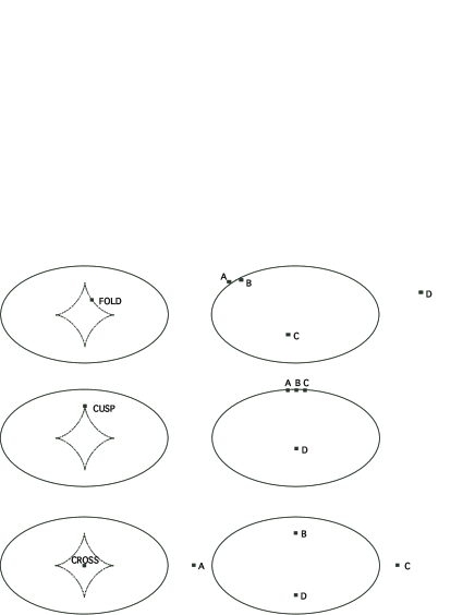
Figure 1: The three types of image configurations: folds (top right), cusps (middle right), and crosses (bottom right), with the corresponding source position and caustic curve to the left. The lens potential used here is an SIE with ellipticity $e=0.5$.

A similar magnification relation holds when the source lies near a fold caustic (see Fig. 1). In this case, two of the four images lie closely-spaced together, straddling the critical curve (the so-called fold image pair). One of these images is a minimum and the other a saddle. When the source lies asymptotically close to the fold caustic, the fold image pair should satisfy $|\mu_{\rm{min}}|-|\mu_{\rm{sad}}|\approx 0$. For four-image lenses, Keeton et al. (2005) used this relation to define

$$R_{\rm{fold}}\equiv{|\mu_{\rm{min}}|-|\mu_{\rm{sad}}|\over|\mu_{\rm{min}}|+|\mu_{\rm{sad}}|}={F_{\rm{min}}-F_{\rm{sad}}\over F_{\rm{min}}+F_{\rm{sad}}}\cdot$$ (3)

Like its predecessor, the ideal fold relation $R_{\rm{fold}}\to 0$ is satisfied only when the source lies asymptotically close to the fold caustic. To move beyond the asymptotic regime, these authors expanded the lens mapping in a Taylor series about the fold point to get

$$R_{\rm{fold}}=0+A_{\rm{fold}}d_{1}+\cdots,$$ (4)

where $d_{1}$ is now the distance between the two images in the fold image pair and the coefficient $A_{\rm{fold}}$ is a function that depends once again on those properties of the lens potential listed above. As we approach a cusp in the asymptotic regime, $|A_{\rm{fold}}|\to\infty$, where the sign depends on whether the cusp is on the long or short axis of the caustic. For a cusp on the long axis, $A_{\rm{fold}}\to-\infty$ because the middle image is a saddle, whereas for a cusp on the short axis, $A_{\rm{fold}}\to+\infty$ because the middle image is a minimum (remember that we are now looking at a cusp triplet, but using $R_{\rm{fold}}$ instead of $R_{\rm{cusp}}$, and that $R_{\rm{fold}}$ is to be evaluated on minimum/saddle pairs of images). This means that $R_{\rm{fold}}$ breaks down asymptotically close to a cusp, which is not too surprising because it is designed to be evaluated only on fold points. We mention this fact because in our calculations below we do indeed evaluate $R_{\rm{fold}}$ for cusp points, but we are safe in doing so because our source sits a small but finite distance from the cusp, and is not asymptotically close.

The more interesting feature of $R_{\rm{fold}}$, as Keeton et al. (2005) discovered, is that the validity of the ideal fold relation depends not just on how close the source is to the fold caustic, but also where precisely the source is along the caustic. This is reflected in the coefficient $A_{\rm{fold}}$, which takes on all values, both positive and negative, as one moves along the caustic (see Fig. 2). For this reason the authors introduced another variable, the distance $d_{2}$ to the next nearest image (note that, as we are dealing with minimum/saddle image pairs only, neither $d_{1}$ nor $d_{2}$ will ever denote the distance between two saddles or two minima). They did so because both the source and the fold caustic are of course unobservable, and therefore the value of $A_{\rm{fold}}$, too, is unknown. Fortunately, the source’s position is encoded in the image configuration: not in the separation $d_{1}$ between the fold image pair, but rather in the distance $d_{2}$ to the next nearest image. (To give an example: a source near a fold but not near a cusp will have $d_{1}\ll d_{2}\sim R_{\rm{E}}$, whereas a source near a cusp will have $d_{1}\sim d_{2}\ll R_{\rm{E}}$, where $R_{\rm{E}}$ is the Einstein radius.) Hence the authors concluded that when deriving an upper bound on $R_{\rm{fold}}$, beyond which one can infer the presence of small-scale structure, $d_{2}$ must also be taken into account along with $d_{1}$. The sensitivity of $R_{\rm{fold}}$ with respect to the source’s position along the fold caustic will unfortunately make things difficult for us, and for this reason we will concentrate on cusp points only, not fold points; see $\S 3$ below.

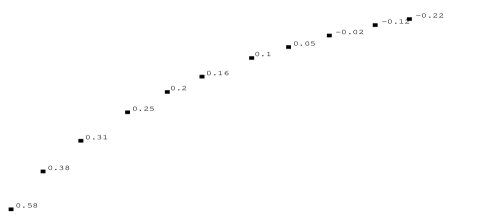
Figure 2: Caustic curve for an SIE with ellipticity $e=0.5$. The numbers below are the values of $A_{\rm{fold}}$ in the asymptotic fold relation $R_{\rm{fold}}=A_{\rm{fold}}d_{1}$, evaluated at the points selected above. Note that $A_{\rm{fold}}$ is monotonically decreasing from left to right, as one moves from the short axis to the long axis. As Appendix A of Keeton et al. (2005) discusses rigorously, $A_{\rm{fold}}$ is to be evaluated on the caustic, but describes the fold relation in the vicinity of the caustic.

Incidentally, in Figures 1 and 2, and in all of our calculations below, we use as our lens model an SIE with ellipticity $e=0.5$. Although we are restricting our theoretical analysis to an SIE, our results are nevertheless general, for the following reason. Keeton et al. (2005) generated a large ensemble of realistic lens potentials drawn from three different observational samples, with varying values of ellipticity, octupole modes, and external shear. For each lens potential in their ensemble, they chose $\sim 10^{6}$ source positions, solved the lens equation using Gravlens, and then computed $(d_{1},d_{2},R_{\rm{fold}})$ for each minimum/saddle image pair. They then plotted $R_{\rm{fold}}$ on the $(d_{1},d_{2})$ plane. This enabled them to extract the probability distribution of $R_{\rm{fold}}$ for fixed values of $d_{1}$ and $d_{2}$. Next, using an SIE with $e=0.5$, they chose source positions such that $d_{1}^{\rm{fold}}=d_{1}^{\rm{cusp}}=.46R_{\rm{ein}}$, and calculated $R_{\rm{fold}}$. They compared this value of $R_{\rm{fold}}$ to that of each of the lens potentials in their ensemble, for the same values of $d_{1}$ and $d_{2}$. Finally, for each minimum/saddle image pair, they found that the value of $R_{\rm{fold}}$ calculated in the case of the SIE fell within the probability distribution of their ensemble, and thus concluded that each image pair of the SIE was consistent with lensing by a realistic potential. They repeated this procedure on the 23 known four-image lenses, and concluded that each case in which $R_{\rm{fold}}$ lay outside the probability distribution constituted strong evidence that small-scale structure was present for that particular lens. Given their result, we take as our ‘archetypal smooth lens potential’ an SIE with ellipticity $e=0.5$. However, we also vary the ellipticity and external shear and evaluate their impact on our results.

3 Investigating $R_{\rm{cusp}}$ and $R_{\rm{fold}}$

Prior to adding our point-mass substructures to the SIE, we calculate the values for $R_{\rm{cusp}}$ and $R_{\rm{fold}}$ for a smooth lens model. In what follows, we assume that the source sits a very small but finite distance from the cusp or the fold.

For a source near a fold caustic but not near a cusp (mathematically, this means that we pick a neighborhood around our source that does not contain a cusp point), the image configuration is given in the top panel of Fig. 1. Calculating $R_{\rm{fold}}$ for the fold image pair (A,B) that straddles the critical curve gives $R_{\rm{fold}}\approx 0$ because, as stated in §2, A & B have roughly equal and opposite magnifications. Of course we can apply $R_{\rm{fold}}$ to any minimum/saddle image pair. Now, the two fold pair images A & B will have much higher magnifications than the other two images C & D. In fact, it can be as much as three orders of magnitude greater. So the fold relation for an image in the fold image pair and one of the other two images will converge to $R_{\rm{fold}}\approx\pm 1$. If the image in the fold image pair is a minimum, we get $+1$; if it is a saddle, we get $-1$.

The more interesting case is when a source lies near a cusp point, in which case we can use both relations $R_{\rm{cusp}}$ and $R_{\rm{fold}}$; see the middle panel of Fig. 1. In this case the magnifications of the outer two images A & C will have the same sign and exactly the same magnitude, while the magnification of the middle image B will have the opposite sign and roughly twice the magnitude, with the sign depending on whether the source lies near a long axis cusp (B is a saddle) or near a short axis cusp (B is a minimum). Of course, as stated in $\S 2$, for the cusp triplet (A,B,C), $R_{\rm{cusp}}\approx 0$. We now apply $R_{\rm{fold}}$ to the cusp triplet. Pairing the middle image B with either of the outer images A or C gives $R_{\rm{fold}}\approx\pm 1/3$. If B is a saddle, then A & C are minima, so we get $-1/3$; if B is a minimum, then A & C are saddles, and we get $+1/3$. The fourth image D, not part of the cusp triplet, will have a magnification much less than that of A,B, or C. It can be as much as three orders of magnitude less. So the fold relation gives $R_{\rm{fold}}\approx\pm 1$ for the combination of any one of the cusp triplet images and D. The sign will depend on which cusp triplet image we use, and whether the source sits on the long or short axis: for a long axis cusp, (A,D) and (C,D) give $+1$, while (B,D) gives $-1$.

Of all these values, the important ones for our purposes are the relations $R_{\rm{cusp}}\approx 0$ and $R_{\rm{fold}}\approx\pm 1/3$ for the cusp triplet: as we will show in the next section, substructure breaks the cusp triplet symmetry. The breaking of the symmetry causes the two outer images to no longer have identical magnifications (and thus the same value for $R_{\rm{fold}}$). They are also no longer equidistant from the middle image.

4 Simulating the effects of substructure

Since our examination involves a simulated configurations rather than observational data, we can and choose to keep the source position fixed and investigate the effect of substructure on the image configurations. Specifically, we investigate the change to both the image configurations and to the values of $R_{\rm{fold}}$ and $R_{\rm{cusp}}$ when we distribute substructure in the form of point-masses onto our archetypal smooth lens potential, an SIE with ellipticity $e=0.5$. We consider both random and symmetric spatial distributions for 5-10 point-masses. We examine cases when the spatial distribution of these point-masses is (1) less than, (2) roughly equal to, and (3) greater than the distance between the images. We use Gravlens to solve the modified lens equation (SIE + point-masses) for a source placed very close to either a fold or cusp. In each case, we gradually increase the mass of our point-masses from $0$ (the control case) to the ‘cut-off’ mass, which is the mass value beyond which we no longer have a four-image lens. Finally, we calculate $R_{\rm{fold}}$ and $R_{\rm{cusp}}$ for these granular lenses.

When considering sources near a cusp, we concentrate on long axis cusps because they satisfy the ideal fold relation more readily than short axis cusps (Keeton et al. 2005). We also ignore cross configurations (see the bottom panel of Fig. 1) because in such a case $d_{1}\sim d_{2}\sim R_{\rm{E}}$, and scales on the order of the Einstein radius are no longer ‘small-scale’. (Recall from $\S 2$ above that a violation of the cusp or fold relation implies the presence of significant substructure on scales smaller than the distance between the images. Therefore calculating $R_{\rm{fold}}$ for widely separated images does not really tell us about small-scale structure, because we are no longer restricted to short length scales.)

Of course, the shortest length scale (i.e. the smallest possible value for $d_{1}$) is the distance between the fold image pair in a fold image configuration (the two closely-spaced images in the top panel of Fig. 1). However, we encounter a problem when investigating sources near a fold but not near a cusp. In general, changing the lens potential by adding substructure changes the shape of the caustic curve, and the nature of the change depends on both the spatial distribution of the substructure, and more importantly, their masses. To give an example: setting the mass of our SIE to 1 (this sets $R_{\rm{E}}=1$ in the code units), the spatial distribution of five point-masses in the manner shown in Fig. 3, with masses ranging from $0<m_{i}\leq 0.0190$, deforms the caustic curve considerably, but still produces four-image lenses. For masses $0.0190\leq m_{i}<0.0259$, the lens can also produce five images, though the fifth image is quite faint: its magnification is $|\mu|\sim 10^{-5}$, while $|\mu|$ for any one of the cusp triplet images is $\sim 10^{2}$. Finally, for masses $m_{i}\geq 0.0259$, the lens can produce six images. Strictly speaking, the cusp and the fold relations are defined only for four-image lenses, so we will not examine $R_{\rm{cusp}}$ and $R_{\rm{fold}}$ in the five- and six-image regimes.

We would like to come as close as we can to satisfying the ideal fold and cusp relations, we want to place our source as close to the caustic curve as Gravlens allows. Now, aside from deforming certain regions of the caustic curve, the addition of substructure also tends to narrow the diamond-shaped region of the curve, so that a source placed very close to a fold or cusp may actually end up falling outside the diamond-shaped region of the new caustic curve. A source outside this region, of course, will not produce fold or cusp configurations, so this means that we are forced to move our source back inside the diamond-shaped region of our new caustic curve in order to produce four-image configurations. We do encounter the problem of trying to place our new source in the ‘same place’ with respect to the new fold caustic as our old source was with respect to the old fold caustic. Given the sensitivity of $R_{\rm{fold}}$ to where our source lies along the fold (see §2 and Fig. 2), this is difficult in practice. When we move our source back inside the caustic curve, the value of $R_{\rm{fold}}$ will change, but we cannot say with confidence whether this change in $R_{\rm{fold}}$ is due to the addition of substructure, or simply because we displaced our source by a small amount. For this reason, we ignore sources lying near a fold.

Figure 3: The breaking of the cusp triplet symmetry for a distribution of five point-masses onto an SIE with ellipticity $e=0.5$. In each panel, the diagram on the left shows the caustic curve and source position while that on the right shows the corresponding critical curve and cusp configuration. For each caustic curve we have moved our source as close to the cusp as Gravlens allows. In each case, note the deformations of both the caustic and critical curves due to the point-masses, and compare these with the cusp configuration in Fig. 1. The triangles are the point-masses and the squares are the images. In each panel, the point-masses have the same mass. In the first panel, that mass is $m=0.0185$ (in units where $R_{\rm{E}}=1$); in the second panel, $m=0.0255$; in the third, $m=0.0258$. Note the fifth image near the origin in the second and third rows. For $m\geq 0.0259$, we get six images.

Fortunately, we do not encounter this problem when we place our source near a cusp, because the cusp is a much smaller region than the fold caustic. We cannot ‘move along’ the cusp in the same way that we can move along the fold because the cusp is essentially a tiny wedge. Therefore we can safely move our source back inside the caustic curve and place it back into the wedge of the cusp. We still have to be careful, however, because the addition of substructure tends to displace the long axis cusp slightly off the axis (so that the long axis is no longer aligned with the coordinate axis), making it more difficult to locate the cusp accurately. Doing so gives us our most interesting result: when we add substructure onto our SIE, and consider a source near our new long axis cusp, we no longer have the symmetry in our cusp triplet. The cusp triplet tends to be displaced to one side, so that the two outer images are no longer identical. In fact, one of them is closer to the middle image. This is illustrated in the three panels shown in Fig. 3. At this point an important issue arises: because the cusp point is more difficult to locate when substructure displaces the long axis, one may wonder whether the skewed cusp triplet shown in Fig. 3 is caused merely by the possibility that we have missed the cusp point and instead placed our source against a fold caustic. If so, then we would be able to reproduce the same skewed cusp triplet in the case of an SIE without substructure, simply by displacing our source off the cusp by a small amount. But in fact this is not the case: a source displaced slightly off the cusp for an SIE without substructure produces a very tight fold configuration (as in the top panel of Fig. 1), one that looks altogether different from the skewed cusp triplet shown in Fig. 3. Thus it is the substructure that breaks the cusp triplet symmetry.

5 Results and Conclusions

We now examine the sensitivity of the cusp and the fold relations to the spatial distribution of substructure shown in Fig. 3. We set the mass of our SIE to 1 ($R_{\rm{E}}=1$) and vary the substructure masses from $0$ (the control case) to $m_{i}=0.019$. For a typical galaxy lens this corresponds to adding substructure in the mass range of 10⁵ - 10${}^{7}\,M_{\odot}$. Note that for $m_{i}>0.019$ we no longer have a four-image lens.

5.1 Dependence on Substructure Mass

First of all, for the control case of the smooth potential and no substructure, we find $R_{\rm{cusp}}=0.002$ and $R_{\rm{fold}}=(-0.331,-0.331)$, where $R_{\rm{fold}}=-0.331$ for both the left/middle image pair and the right/middle image pair. As discussed in $\S 3$, we expect a value close to $0$ for $R_{\rm{cusp}}$ because we have placed our source as close to the cusp as Gravlens allows (see Fig. 1). However, our source still sits a finite distance from the cusp, not asymptotically close, so we should not expect to satisfy the ideal cusp relation $R_{\rm{cusp}}\to 0$ exactly; hence $R_{\rm{cusp}}=0.002$ is acceptably close to zero. As for $R_{\rm{fold}}=-0.331$, this value, too, is what we expect: both the leftmost and rightmost images have the same magnification, which is half the magnitude as that of the middle image with the opposite sign. In this case our source sits near a long axis cusp, so the middle image is a saddle and $R_{\rm{fold}}$ is negative. As discussed in $\S 3$, we expect a value of $R_{\rm{fold}}\approx-0.333$, so a value of $-0.331$ is close enough.

Now we examine the breaking of the cusp triplet symmetry shown in Fig. 3, for three mass values in the four-image regime:

• $m=.000$ : $R_{\rm{cusp}}=.002$ and $R_{\rm{fold}}=(-.331,-.331)$

• $m=.001$ : $R_{\rm{cusp}}=.005$ and $R_{\rm{fold}}=(-.326,-.332)$

• $m=.005$ : $R_{\rm{cusp}}=.006$ and $R_{\rm{fold}}=(-.317,-.340)$

• $m=.010$ : $R_{\rm{cusp}}=.006$ and $R_{\rm{fold}}=(-.305,-.352)$

The notation $R_{\rm{fold}}=(-0.317,-0.340)$ implies that the left/middle image pair gives $R_{\rm{fold}}=-0.317$, while the right/middle image pair gives $R_{\rm{fold}}=-0.340$; likewise for the others. The change in $R_{\rm{fold}}$ manifestly reveals the breaking of the cusp triplet symmetry; the change in $R_{\rm{cusp}}$, however, does not, as shown in the top panel of Fig. 4. In Fig. 4 we show the effect of varying the mass of the substructure on $R_{\rm{cusp}}$ and $R_{\rm{fold}}$. It is clear that, within the four-image regime, $R_{\rm{fold}}$ readily reflects the change in the mass of the substructure, while $R_{\rm{cusp}}$ stays roughly constant.

Figure 4: $R_{\rm{cusp}}$ and $R_{\rm{fold}}$ as a function of the mass $m$ of the substructure for the $e=0.5$ case, for the spatial distribution given in Fig. 3. Left column: Without shear. For $0\leq m\leq 0.0185$ (in units where $R_{\rm{E}}=1$), we get four images for a source as near the long axis cusp as Gravlens allows. Right column: External shear with an amplitude of $\gamma\sim 5\%$. In this case we have a four-image regime for $0\leq m\leq 0.020$. The control case (no substructure) is shown by the dashed line. In the bottom panel, the black and white data points denote the left/middle and right/middle image pairs in the cusp triplet, respectively. $R_{\rm{fold}}$ reflects the change in the mass of the substructure better than $R_{\rm{cusp}}$.

Keeton et al. (2005) demonstrated that, for observed cusp lenses, the fold relation indicated the same flux ratio anomalies as the cusp relation, with one exception: in B2045+265, the possible presence of octupole modes precluded the authors from declaring that the fold relation was violated, whereas the cusp relation was very clearly violated. However, because the fold relation is defined for pairs, it gave the additional information of indicating which particular image in the cusp triplet was the one most affected by substructure, a distinction that could not be made with the cusp relation. What we have shown in our analytic argument here is that, for an SIE with $e=0.5$, the fold relation is a more reliable indicator of substructure than the cusp relation.

5.2 Sensitivity to External Shear

Both $R_{\rm{cusp}}$ and $R_{\rm{fold}}$ are expected to be sensitive to the presence of external shear. We therefore add external shear with an amplitude of $\gamma\sim 5\%$ to the configurations. With this modification, we examine the breaking of the cusp triplet symmetry for the same substructure mass values listed in §4.1, and find:

• $m=.000$ : $R_{\rm{cusp}}=.005$ and $R_{\rm{fold}}=(-.329,-.329)$

• $m=.001$ : $R_{\rm{cusp}}=.006$ and $R_{\rm{fold}}=(-.326,-.330)$

• $m=.005$ : $R_{\rm{cusp}}=.006$ and $R_{\rm{fold}}=(-.318,-.338)$

• $m=.010$ : $R_{\rm{cusp}}=.006$ and $R_{\rm{fold}}=(-.311,-.346)$

Once again, $R_{\rm{fold}}$ manifestly reveals the breaking of the cusp triplet symmetry, whereas $R_{\rm{cusp}}$ does not. In fact, as Fig. 4 shows, $R_{\rm{cusp}}$ eventually falls below the control case value of $R_{\rm{cusp}}=0.005$. On the other hand, $R_{\rm{fold}}$ remains correlated with the mass of the substructure throughout the four-image regime, even with external shear. Finally, note that the four-image regime in this case is produced when $m_{i}<0.02$.

5.3 Sensitivity to Ellipticity

The ellipticity of our SIE affects the values of $R_{\rm{cusp}}$ and $R_{\rm{fold}}$. We find that for ellipticities lower than our archetypal value of $e=0.5$, $R_{\rm{cusp}}$ remains unresponsive to the substructure, whereas $R_{\rm{fold}}$ is still sensitive to the mass of substructure, though not as robustly as for the case with $e=0.5$. The left-hand panels of Fig. 5 demonstrates this explicitly for an ellipticity $e=0.25$. For ellipticities higher than our archetypal value, $R_{\rm{cusp}}$ displays erratic fluctuations, whereas $R_{\rm{fold}}$ remains well correlated with the mass of the substructure, as shown in the right-hand panels of Fig. 5.

Figure 5: Left column: $R_{\rm cusp}$ and $R_{\rm fold}$ as in Fig.  4, but now for a lens with ellipticity $e=0.25$. We have a four-image regime for $0\leq m\leq 0.009$. We ignore the region $0<m<0.002$ because it is difficult to cleanly place the source near the cusp point. Right column: The relations for a lens ellipticity $e=0.75$. In this case we have a three-image regime (a cusp triplet, no fourth image) for $0\leq m\leq 0.035$, and four-image regime for $0.035<m\leq 0.100$. Note that although $R_{\rm{cusp}}$ fluctuates erratically, in this case the right/middle image pair of $R_{\rm{fold}}$ is not reliable, either. The most reliable indicator of the substructure masses here is the left/middle image pair of $R_{\rm{fold}}$.

5.4 Concluding remarks

In this theoretical investigation, we attempt to develop a robust diagnostic that quantifies the presence of substructure in lens galaxies. To this end, we simulated a simple lens potential with added substructure, with the aim of seeing how the cusp and the fold relations, calculated while keeping the source position fixed, respond to the presence of the substructure as we vary its mass and position within the lens. We took as our lens model an SIE and used point-masses as our substructure with masses ranging from $0<m_{i}\leq 0.019$ ($R_{\rm{E}}=1$). When we varied the ellipticity of our SIE, we found that for low ellipticities the cusp relation was unresponsive to the substructure, whereas for high ellipticities it became erratic. The fold relation, on the other hand, remained well correlated with the mass of the substructure. Considering the effect of external shear gave the same result: the fold relation remained well correlated with the substructure, whereas the cusp relation did not.

We considered random distributions of point-masses as substructure and cases when their spatial distribution was less than, roughly equal to, and greater than the distance between the images. Overall, we found that the addition of substructure breaks the symmetry of the cusp triplet, and that the fold relation responds more accurately to the change in mass of the substructure than the cusp relation. We conclude, therefore, that the fold relation is the more robust diagnostic of substructure.

In order to apply this technique to real data, we will need to use the observed image positions and the distances between them, and then use Monte Carlo methods to constrain the corresponding source positions. While this is beyond the scope of this work, we pursue it in a follow-up paper.

References

- [1] Blandford, R. & Narayan, R. 1986, ApJ, 310, 568
- [2] Chiba, M., Minezaki, T., Kashikawa, N., Kataza, H., & Inoue, K.T. 2005, ApJ, 627, 53
- [3] Dalal, N. & Kochanek, C.S. 2002, ApJ, 572, 25
- [4] Diemand, J., Moore, B., & Stadel, J. 2005, Nature, 433, 389
- [5] Fassnacht, C.D., et al. 1999, AJ, 117, 658F
- [6] Gaudi, B.S. & Petters, A.O. 2002a, ApJ, 589, 688
- [7] Gaudi, B.S. & Petters, A.O. 2002b, ApJ, 580, 468
- [8] Inada, N., et al. 2003, AJ, 126, 666
- [9] Jackson, N., et al. 1998, MNRAS, 296, 483J
- [10] Keeton, C.R. 2001, astro-ph/0102340
- [11] Keeton, C.R., Gaudi, B.S., & Petters, A.O. 2003, ApJ, 598, 138
- [12] Keeton, C.R., Gaudi, B.S., & Petters, A.O. 2005, ApJ, 635, 35
- [13] Mao, S. & Schneider, P. 1998, MNRAS, 295, 587
- [14] Mathis, H., Lemson, G., Springel, V., Kauffmann, G., White, S.D.M., Eldar, A., & Dekel, A. 2002, MNRAS, 333, 739
- [15] Metcalf, R.B. & Madau, P. 2001, ApJ, 563, 9
- [16] Moore, B., Ghigna, S., Governato, F., Lake, G., Quinn, T., Stadel, J., & Tozzi, P. 1999, ApJ, 524, 19
- [17] Patnaik, A.R., Kemball, A.J., Porcas, R.W., & Garrett, M.A. 1999, MNRAS, 307, L1
- [18] Petters, A.O., Levine, H., & Wambsganss, J. 2001, Singularity Theory and Gravitational Lensing (Boston: Birkhäuser)
- [19] Refsdal, S. 1964, MNRAS 128, 295
- [20] Schneider, P., Ehlers, J., & Falco, E.E. 1992, Gravitational Lenses (Berlin: Springer)
- [21] Schneider, P. & Weiss, A. 1992, A&A, 260, 1